Land-Use and Land-Cover Classification Using a Human Group-Based Particle Swarm Optimization Algorithm with an LSTM Classifier on Hybrid Pre-Processing Remote-Sensing Images

Abstract

Land-use and land-cover (LULC) classification using remote sensing imagery plays a vital role in many environment modeling and land-use inventories. In this study, a hybrid feature optimization algorithm along with a deep learning classifier is proposed to improve the performance of LULC classification, helping to predict wildlife habitat, deteriorating environmental quality, haphazard elements, etc. LULC classification is assessed using Sat 4, Sat 6 and Eurosat datasets. After the selection of remote-sensing images, normalization and histogram equalization methods are used to improve the quality of the images. Then, a hybrid optimization is accomplished by using the local Gabor binary pattern histogram sequence (LGBPHS), the histogram of oriented gradient (HOG) and Haralick texture features, for the feature extraction from the selected images. The benefits of this hybrid optimization are a high discriminative power and invariance to color and grayscale images. Next, a human group-based particle swarm optimization (PSO) algorithm is applied to select the optimal features, whose benefits are a fast convergence rate and ease of implementation. After selecting the optimal feature values, a long short-term memory (LSTM) network is utilized to classify the LULC classes. Experimental results showed that the human group-based PSO algorithm with a LSTM classifier effectively well differentiates the LULC classes in terms of classification accuracy, recall and precision. A maximum improvement of 6.03% on Sat 4 and 7.17% on Sat 6 in LULC classification is reached when the proposed human group-based PSO with LSTM is compared to individual LSTM, PSO with LSTM, and Human Group Optimization (HGO) with LSTM. Moreover, an improvement of 2.56% in accuracy is achieved, compared to the existing models, GoogleNet, Visual Geometric Group (VGG), AlexNet, ConvNet, when the proposed method is applied.

1. Introduction

In recent years, land-use and land-cover (LULC) classification using remote-sensing imagery plays an important role in many applications like land use planning (growth trends, suburban sprawl, policy regulations and incentives), agricultural practice (conservation easements, riparian zone buffers, cropping patterns and nutrient management), forest management (harvesting, health, resource-inventory, reforestation and stand-quality) and biological resource (fragmentation, habitat quality and wetlands) [1,2,3]. Land use refers to the purpose the land serves and land cover refers to the surface cover on the ground, whether vegetation, urban infrastructure, water, bare soil or other; it does not describe the use of land, and the use of land may be different for lands with the same cover type [4,5]. LULC assessment is very necessary in sustaining, monitoring and planning the usage of natural resources [6,7]. In fact, LULC classification has a direct impact on atmospheric, soil erosion and water, while it is indirectly connected to global environmental problems [8,9]. At this end, the remote sensing imagery and its processing has helped in delivering up-to date and large-scale information on surface conditions.

For years, techniques mainly based on pixel or object analysis have been used for LULC classification. An object-based technique usually outperforms a pixel-based one, as demonstrated in [10,11,12]. In fact, unlike the pixel-based technique, which classifies the pixels according to their spectral information, the object-based algorithms enclose semantic information not in the individual pixel but in groups of pixels with similar characteristics, such as color, texture, brightness and shape. Both the spatial and spectral resolution are used in this latter case to segment and then classify image features into meaningful objects [13]. From the resulting segments, homogeneous image objects are extracted based on the local contrast. These homogeneous objects are then classified using traditional classification approaches such as the nearest neighbor, or using knowledge-based approaches and fuzzy classification logic [14].

Recently, studies in literature have moved towards data integration in order to improve the accuracy of urban LULC classification [15,16]. Data integration refers to the integration of information from various sources or sensors, such as the integration of LiDAR and optical data, for instance [17,18,19]. Nevertheless, even these techniques used in LULC classification present some issues since they are extremely affected by the environmental changes, like destruction of essential wetlands, uncontrolled urban development, haphazard, loss of prime agricultural lands, deteriorating environmental quality, and also by other factors, like cloud cover and regional fog errors. Moreover, traditional remote-sensing imagery processing offers some other concerns: the noise associated with the image, the orientation of features in the images and the maintenance of a large volume of data [19,20]. Several methodologies have been developed by the researchers to address those issues faced in LULC classification. Examples of these methodologies are adaptive reflectance fusion models, maximum likelihood classifiers, decision trees, convolutional neural networks (CNNs), deep neural networks (DNNs), etc. [21,22,23,24,25]. In some cases, DNNs are also used for pre-trained the data, in other cases the image classification for LULC is accomplished via more complex machine learning (ML) algorithms. It is worth to highlight that ML algorithms have gained ground in recent years also because they resulted to be more suitable to realize unsupervised, or semi-automatic classification systems, with huge amounts of data.

With respect to recent works presented in the literature [26,27,28], the study presented in this article has proposed a new algorithm, a human group-based particle swarm optimization (PSO) algorithm, with a long short-term memory (LSTM) classifier, to address the aforementioned issues and improve LULC classification, in agriculture and urban environments. Remote-sensing images are retrieved from Sat 4, Sat 6 and Eurosat datasets, also used in [26,27,28], but better results are reached with the new algorithm, as shown ahead in this manuscript. In particular, a maximum improvement of 6.03% on Sat 4 and 7.17% on Sat 6 in LULC classification is reached when the proposed human group-based PSO with LSTM is compared to individual LSTM, PSO with LSTM, and Human Group Optimization (HGO) with LSTM. Moreover, an improvement of 2.56% in accuracy is achieved compared to the existing models GoogleNet, Visual Geometric Group (VGG), AlexNet, ConvNet, when the proposed method is applied.

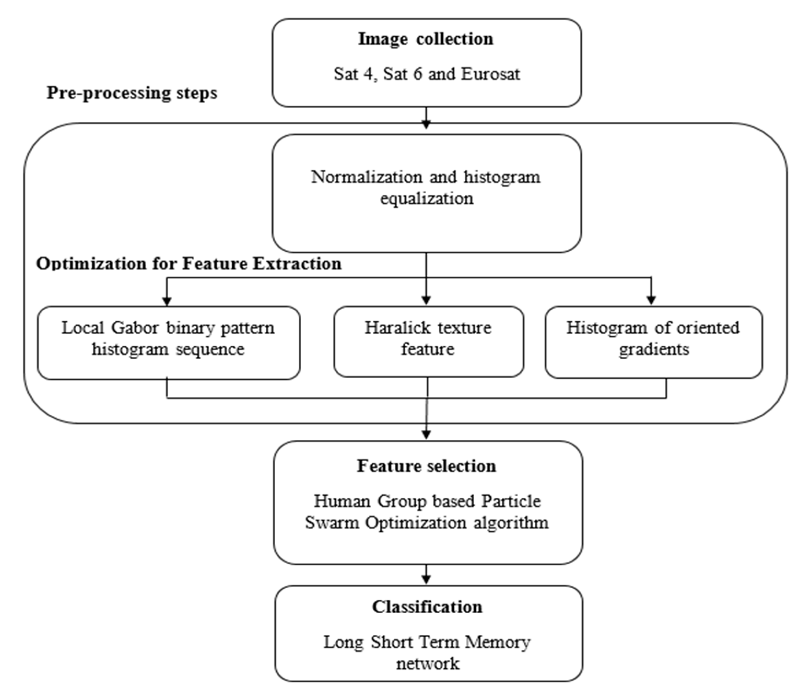
The general architecture of the proposed algorithm and the several detailed processing steps are presented and explained in detail in the Section 3, but here the summary of the main operations is given. In particular, after the selection of the remote-sensing images, normalization and histogram equalization methods are applied to improve the visual quality of the objects. The pre-processing techniques undertaken effectively improve the contrast of the images and enhance the edges in each region of the image. After normalization, feature extraction is carried out by using the local Gabor binary pattern histogram sequence (LGBPHS), the histogram of oriented gradient (HOG) and the Haralick texture features [29,30,31,32]. The LGBPHS is utilized as a two-dimensional spatial image gradient measurement to emphasize the high spatial frequency regions based on the image edges. In addition, it is utilized to identify the absolute gradient scales at each point in a remote sensing image. Next, HOG and Haralick texture features are applied to extract the texture and color feature vectors from the image pixels. As the HOG feature descriptor operates on local cells, it is invariant to photometric and geometric transformations, which helps in attaining a better classification. The textural properties are calculated by Haralick texture features in order to understand the edge details about the image content. Then, the human group-based PSO algorithm is used to select the optimal feature vectors that significantly reduces the “curse of dimensionality” issue. The optimal feature vectors obtained are given as the input to the LSTM classifier to establish the LULC classes. In the result section, the performance of the proposed human group-based PSO with LSTM is evaluated in terms of recall, precision and classification accuracy and compared with other existing models such as GoogleNet, VGG, AlexNet and ConvNet.

This research paper is organized as follows. Section 2 presents several existing research papers on the LULC topic, when advanced methodologies, such as HOG, LGBPHS, ML, ML in combination with object-based image analysis (OBIA), bag-of-visual words (BOVW) and scale-invariant feature transform (SIFT) methodologies are used. In Section 3, the proposed model is explained in detail with mathematical expressions. Experimental analysis of the proposed model is then presented and discussed in the Section 4. Conclusions of this study are drawn in Section 5

2. Literature Survey

As already highlighted, advanced methodologies have gained ground in recent years to overcome unsolved issues of traditional methods, and because more suitable to realize unsupervised, or semi-automatic classification systems, which require a huge amount of data. This section aims to present an extensive survey of related papers.

A new rotationally invariant feature descriptor has been developed by Xiao et al. [33] to identify cars and aircraft in the remote-sensing images. The rotationally invariant HOG descriptor used elliptic Fourier transform, orientation normalization and feature space mapping to achieve better performance in object detection from remote-sensing images. In [34] Rahmani and Behrad developed a new automatic model for ship detection in the remote-sensing images. Initially, the collected images were divided into overlapping blocks and then the LGBPHS feature descriptor was used to extract the features from the images. Support vector machine (SVM) and artificial neural network (ANN) were used for classification after feature extraction. However, SVM supports only binary classification, which is not adaptable for multiclass classification.

Kadavi and Lee [35] used SVM and ANN classifiers to evaluate the multi-spectral data from mount Fourpeaked, mount Kanaga, mount Augustine and mount Pavlof in the United States of America. In this study, a Landsat-8 imagery dataset was used to evaluate the efficiency and effectiveness of the developed model. The Landsat-8 imagery allowed to derive four land cover classes: vegetation, snow, water bodies and outcrops (sand, volcanic rock, etc.). Simulation results showed that the SVM classifier attained better performance in LULC classification compared to ANN classifier. For mount Kanaga, the SVM classifier achieved maximum classification accuracy, which was 9.1% superior to ANN classifier. However, the developed model was only suitable for minimum class classification, not for maximum class classification, and the developed model showed poor performance in some conditions like cloud cover and regional fog error. Pencue-Fierro et al. [36] presented a new hybrid framework for multi-region, multi-sensor and multi-temporal satellite image classification. In this study, land-cover classification was assessed for the Cauca river region, located in the south-west part of Colombia. After image collection, a Coordination of Information on the Environment (CORINE) land-cover approach was used for extracting the feature vectors from the input image. Next, the extracted features were given as the input to a supervised classifier SVM to decide the land cover classes, like urban-area, paramo, snow, clouds, bare soil, grass-land, planted forest, permanent-crops, natural forest, water-bodies and transitory crops. However, the computational complexity was higher in the developed hybrid framework compared to the other methods.

Phiri et al. [37] evaluated moderate-resolution atmospheric transmission, atmospheric correction, cosine topographic correction and dark object subtraction on a heterogeneous landscape in Zambia. In this study, Landsat OLI-8 with 30 and 15 m spatial resolution images were tested using a combination of random forest classifier [38] and an OBIA [39]. The developed method significantly improved land cover classification along with topographic corrections and pan-sharpening atmosphere. The developed framework (random forest and OBIA) effectively classified eight land-cover classes: water bodies, grassland, secondary-forests, dry-agriculture, primary forests, irrigated crops, settlements and plantation-forests. Yet, this study did not concentrate on the feature extraction that may degrade the performance of land-cover classification.

Zhao et al. [40] implemented a new framework for land-use classification using UCMerced land-use dataset and simulated dataset. After collecting the satellite data, BOVW and SIFT [41] methodologies were used for extracting the feature vectors from the collected data. In addition, concentric-circle based spatial rotation-invariant representation was used to describe the spatial information of data. A concentric-circle structured multi-scale BOVW was used for land use classification. The performance of the developed method was analyzed in terms of average classification accuracy. However, the developed method fails to achieve better land use classification in the large datasets due to the “curse of dimensionality” issue.

Nogueira et al. [42] used convolutional neural networks (CNNs) in different scenarios like feature extraction, fine tuning and full training for land cover classification. The developed model’s performance was investigated on three remote sensing datasets: Brazilian coffee scene, UCMerced land-use and remote-sensing “19”. The results indicated that the developed model attained better performance in land cover classification compared to other existing algorithms.

Helber et al. [26] developed a new patch-based LULC classification technique using Eurosat dataset. The undertaken dataset had 13 spectral bands and 10 classes with a total of 27,000 geo-referenced and labeled images. They explained how CNN was used to detect the LULC changes that helped in improving the geographical maps. However, using middle and lower level descriptors, the CNN model leads to poor classification performance because it supports only higher-level descriptors. Unnikrishnan et al. [27] developed a new deep learning model for three different networks VGG, AlexNet and ConvNet where Sat-4 and Sat-6 datasets were used to analyze the performance of the developed model. This model included information on red and near infrared bands, with reduced number of filters, which were tested and trained to classify the images into different classes. The developed model was compared with other networks in terms of trainable parameters, recall and classification accuracy. Papadomanolaki et al. [28] developed a deep learning model based on CNN for precise land-cover classification. The performance of the developed model was compared with the existing networks AlexNet-small, AlexNet and VGG in terms of accuracy and precision on Sat-4 and Sat-6 datasets. However, the CNN had two major concerns: computationally high cost and more data required to achieve precise classification.

Jayanth et al. [43] developed an elephant-herding algorithm to classify LULC regions from high spatial resolution multi-spectral images. The developed elephant herding algorithm achieved high classification accuracy compared to the SVM classifier. Experimental results showed that the elephant-herding algorithm attained better performance in LULC classification on both Arsikere taluk and national institute of technology karnataka (NITK) campus datasets. Extensive experiments showed that the elephant herding algorithm misclassified the dense coconut tree class, which is considered as a major concern in the literature study. Bhosle and Musande [44] developed a CNN model for LULC classification, in particular crop classification, in the hyperspectral remote-sensing images. In this study, the CNN model worked well on unstructured data, where it automatically extracted features for detection and classification of crops. Moreover, the extensive experiment showed that the CNN model achieved effective performance on an Indian pines dataset. However, the CNN model did not encode the orientation and position of objects (crop types) and suffered lack of ability to be spatially invariant to the input data.

Srivastava et al. [45] compared three classification techniques in LULC analysis such as ANN, SVM, and maximum likelihood classification (MLC) to select the best technique among them. In the case of SVM, the classifier was well optimized for the degree of polynomial, penalty, and gamma, where root mean square and minimum output activation threshold were taken into account for ANN. The experimental investigation showed that the ANN classifier was superior to MLC and SVM classifiers. As discussed earlier, ANN classifier is inappropriate for maximum class classification, also showed limited performance in the conditions like regional fog error and cloud cover.

Kindu et al. [46] analyzed LULC changes in the landscape of the Munessa-Shashemene area of the Ethiopian highlands during the period of 1973–2012. The satellite images of Landsat TM (1986), MSS (1973), rapid-eye (2012), and ETM+ (2000) were used to analyze LULC changes. The collected images were classified by using object-based image classifiers. Chatziantoniou et al. [47] combined Sentinel-1 and Sentinel-2 data with the SVM classifier to map LULC on wetlands. In this literature study, the spectral information were derived from minimum noise fraction, grey level co-occurrence matrix, and principal component analysis in order to evaluate the classification accuracy. As stated earlier, the SVM classifier supports only binary classification, which is inappropriate for multiclass classification.

As already highlighted, a human group-based PSO with an LSTM classifier is proposed in this manuscript to address the above-discussed issues and improve the LULC classification, as it will be shown and discussed in the experimental section. It is worth underlining that the proposed model outperforms the methods presented in [26], [27] and [28] as discussed above, which have made use of the same datasets. Hence, a human group-based PSO with a LSTM classifier achieved a minimum of 0.01% and a maximum of 2.56% improvement in classification accuracy on Sat 4, Sat 6 and Eurosat datasets compared to the existing methods presented in [26,27,28].

3. Method

This Section presents the full architecture and all the detailed steps of the proposed algorithm, to allow interested researchers to replicate the image processing. The main workflow of human group-based PSO with an LSTM classifier is shown in Figure 1.

3.1. Image Collection

In this study, Sat 4, Sat 6 and Eurosat datasets are utilized for experimental analysis to differentiate the things that are not related to human habitats in both urban and agricultural environments. The Sat 4 dataset comprises 500,000 image patches with four broad land-cover classes like tree, barren land, grassland and a class with all the other land covers [48,49]. The size of each remote-sensing image in the Sat 4 dataset is $28\times 28$ m. The Sat 6 dataset comprises 40,500 image patches with the size of $28\times 28$ m and it contains six land cover classes grassland like water bodies, buildings, barren land, roads, trees and other classes [27,28]. A sample image of Sat 4 and Sat 6 dataset is presented in Figure 2, and the description of the land-cover classes is given in

Table 1. Description of land-cover classes in Sat 4 and Sat 6 datasets.

Dataset	Classes	Description
Sat 4	Barren land	Barren land includes dry salt flats, sand dunes, deserts, beaches, gravel pits, quarries, exposed rock, strip mines, etc.
	Trees	Forest, a large area of land covered with trees.
	Grassland	Grassland is an area in which the vegetation is dominated by continuous cover of grasses.
	A class that contains all land cover classes other than the above three classes	Includes other land cover classes like wetlands, open water, ice/snow, shrubland, etc.
Sat 6	Barren land	Barren land has sand, rocks, and thin soil, which includes the regions like dry salt flats, sand dunes, deserts, beaches, gravel pits, quarries, exposed rock, strip mines, etc.
	Trees	An area, which is covered with trees, is named as forest.
	Grassland	Grasslands are characterized as lands that are dominated by grasses rather than trees or large shrubs.
	Roads	Human covered areas with hard surface to travel from one place to another place.
	Buildings	Areas for sheltering people, animals, and machinery.
	Water bodies	Presence of standing water surface during most of the year.

.

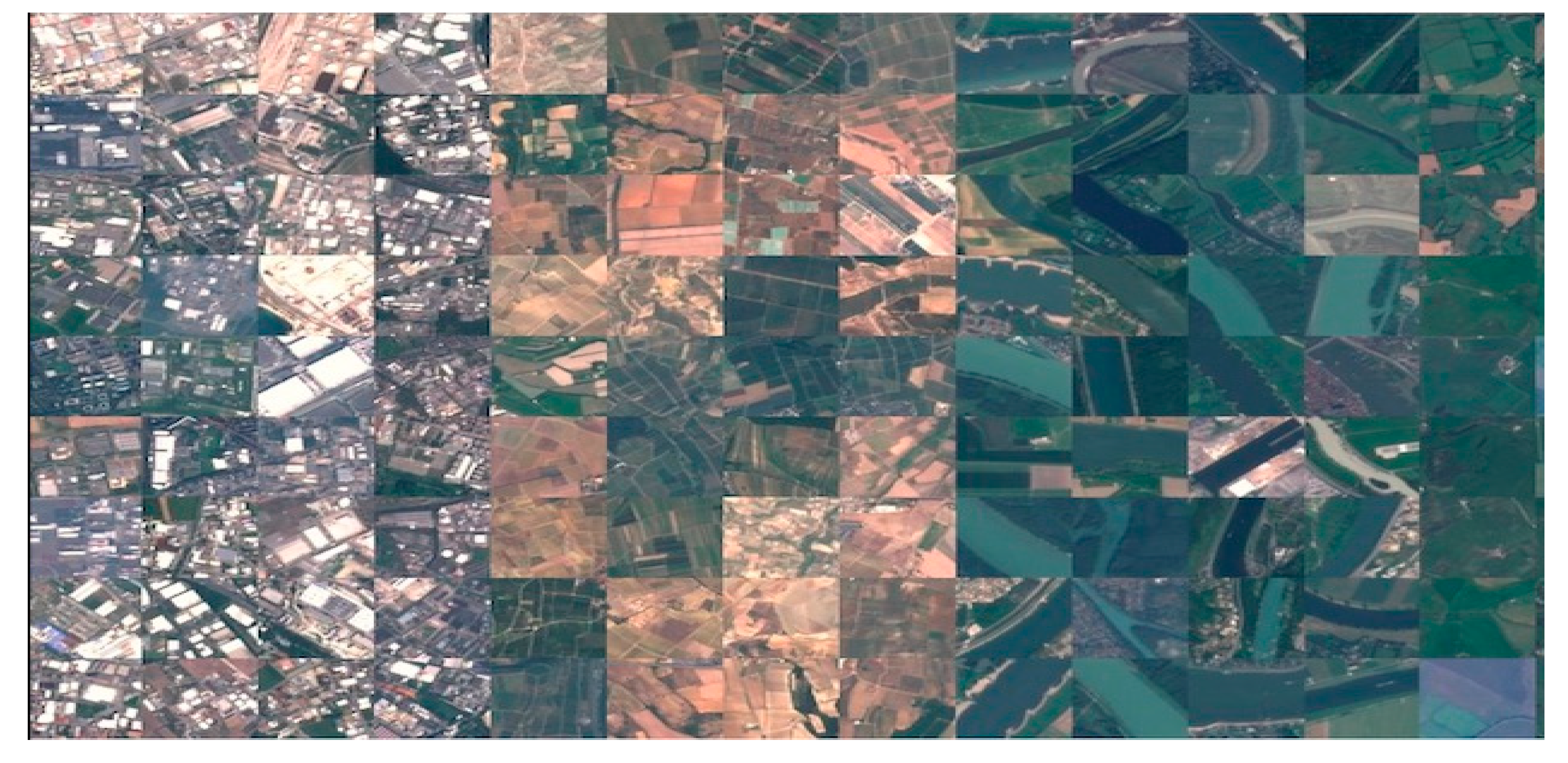
In Eurosat dataset, the satellite images have been captured from European cities, and they are distributed over 34 countries. A dataset is generated with 27,000 labeled and georeferenced image patches, where the size of each image patch is $64\times 64$ m. The Eurosat dataset includes 10 different classes, where each class contains 2000–3000 images. The LULC classes in this dataset are permanent crop, annual crop, pastures, river, sea & lake, forest, herbaceous vegetation, industrial building, highway and residential building [26]. In addition, Eurosat images include 13 bands like aerosols, blue, green, red, red edge 1, red edge 2, red edge 3, near infrared, red edge 4, water vapor, cirrus, shortwave infrared 1 and shortwave infrared 1. A sample image of the Eurosat dataset is presented in Figure 3, and the description of land use and land cover classes in Eurosat dataset is given in

Table 2. Description of land-use and land-cover (LULC) classes in Eurosat dataset.

Dataset	Classes	Description
Eurosat	Permanent crop	Permanent crop occupies the soil and yield harvests for several consecutive years. For example; fruit orchards, vineyards or olive groves, etc.
	Annual crop	Annual crop occupies the soil and yield harvests for limited months. For example; barley, maize, etc.
	Pastures	Pasture is a land used for domesticated livestock like cattle, horses, sheep, etc.
	River	River is a natural flowing watercourse, which flow towards ocean, sea, and lake.
	Sea &lake	A particular area, which is surrounded by water.
	Forest	A large area of land covered with trees.
	Herbaceous vegetation	Areas with herbaceous plants, which are also called as vascular plants that have no persistent woody stems above ground.
	Industrial building	Human covered areas to shelter machinery.
	Highway and residential building	Human covered areas for their own sheltering and travelling.

. In addition, we have indicated the websites in the reference section, where the datasets can be downloaded [50,51]. Interested researchers can follow the described steps to replicate the algorithm.

The Sat 4, Sat 6, and Eurosat datasets are used in this manuscript, as highlighted at the beginning of this section, for experimental analysis to differentiate the things that are not related to human habitats, in both urban and agricultural environments. Future work will extend the proposed analysis to other applications, including human habitats.

3.2. Image Pre-Processing

After collecting the satellite images, normalization and histogram equalization methods are undertaken to improve the quality of the images. Image normalization, also called contrast stretching, changes the range of the pixel values helping in improving the visual quality of the collected satellite images. The common case of a min-max normalization to a new image ranging from 0 to 1, results in the well-known simplified formula expressed by the Equation (1).

$$I_{out}=(I_{in}-Min)\frac{newMax-newMin}{Max-Min}+newMin$$

(1)

where, original satellite image is indicated as $I_{in}$, minimum and maximum intensity values are represented as $Min\hspace{0.17em}\mathrm{and}\hspace{0.17em}Max$ respectively, which ranges from 0 to 255, the image after the min-max normalization is indicated with $I_{out}$, and the new minimum and maximum values are indicated with $NewMin\hspace{0.17em}\mathrm{and}\hspace{0.17em}newMax$. Then, the histogram equalization technique is used to improve the image quality without losing the image information like edges, image patches and points [52,53]. The histogram equalization technique changes the mean brightness of the normalized images to the mid-level of the permitted range, where the preservation of the original brightness avoids annoying artifacts in the images.

3.3. Feature Extraction

After normalization and histogram equalization of the collected satellite images, feature extraction is carried out by using a hybrid optimization procedure, based on the joint use of HOG, LGBPHS and Haralick texture features, namely correlation, contrast, energy, homogeneity, inverse diverse moment, entropy and angular second moment, to extract the feature vectors from the images.

3.3.1. HOG

In the satellite image, the HOG feature descriptor significantly captures the gradient and edge structure of the objects, though, it operates in the localized cells, and this upholds invariance to photometric and geometric transformations (except object orientation) [54,55]. This action helps in finding the changes appears in the large spatial regions. Here, a simple gradient operator $K$ is applied to determine the gradient value. The gradient of the image is given by Equation (2), where $x,y$ represents a generic point in the image and the image frames are denoted as $u$.

$$L_x=K\hspace{0.17em}\ast u\hspace{0.17em}(x,y)\hspace{0.17em}\mathrm{and}\hspace{0.17em}{L}_y=K^T\hspace{0.17em}\ast u\left(x,y\right) L_x$$

(2)

The magnitude of the gradients and edge orientation of the point $x,y$ is calculated by following the respective conditions (Equations (3) and (4)),

$$L(x,y)=\sqrt{L_x{(x,y)}^2{L}_y{(x,y)}^2}$$

(3)

$$\theta (x,y)={\tan }^{-1}{L}_v(x,y)/L_x(x,y)$$

(4)

For improving the invariance in illumination and noise, a normalization process is performed after the calculation of histogram values. The normalization is helpful for contrast and measurement of local histogram. In HOG, four different normalizations are used such as L2-norm, L2-Hys, L1-Sqrt and L1-norm. Among these normalizations, L2-norm gives a better performance in object detection. The blocks of normalization in HOG is given by Equation (5),

$$L_{2-norm}:\hspace{0.17em}f=\frac{q}{\sqrt{{‖q‖}_2^2+e^2}}$$

(5)

where, $e$ is assigned as the small positive value, only when an empty cell is taken into account, $J$ is a feature-extracted value, $q$ is the non-normalized vector in histogram blocks, and ${‖q‖}_2^2$ represents the 2-norm of HOG normalization.

3.3.2. LGBPHS

Initially, the pre-processed satellite images are transformed to obtain multiple Gabor magnitude pictures (GMP) using multi-orientation and multi-scale Gabor filters. Then, each GMP is converted into local GMP (LGMP), which is further categorized into non-overlapping rectangular regions with specific histogram and size [56]. The LGMP histogram of all the LGMO maps is combined to form final histogram sequences. Features extracted by LGBPH are robust to illumination variations, because the LGBPH features are invariant to monotonic gray-scale changes.

3.3.3. Haralick Texture Features

The Haralick features are $2\mathrm{n}\mathrm{d}$ order statistics that reflect the overall average degree of correlation between the pixels in different aspects like contrast, energy, inverse difference moment, entropy, homogeneity, correlation and angular second moment. Haralick texture features effectively deliver information regarding the relative position of the neighborhood image pixels in the satellite images that helps in improving LULC classification performance. The texture features are calculated from the texture information that are present in the grey-level co-occurrence matrix (GLCM) [57]. In order to develop a number of spatial indices, Haralick uses the GLCM, because it contains the two neighboring pixels’ relative frequencies in the image. Haralick develops the vast number of textural features by starting with 14 original features that are described in [58], but only seven features are widely used due to their importance for remote-sensing images. For instance, in [59] they showed a better performance with respect to the others, and, therefore, in this study, those seven commonly used features are considered for the processing.

A set of seven different GLCM indicators is described by the following Equations (6)–(12):

$$Energy={\sum }_{\gamma ,\delta }\hspace{0.17em}\phi {\left(\gamma ,\delta \right)}^2$$

(6)

$$Entropy=\hspace{0.17em}\hspace{0.17em}{\sum }_{\gamma ,\delta }\phi \left(\gamma ,\delta \right){\log }_2\phi \left(\gamma ,\delta \right),\hspace{0.17em}\mathrm{or}\hspace{0.17em}0\hspace{0.17em}\mathrm{if}\hspace{0.17em}\phi \left(\gamma ,\delta \right)=0$$

(7)

$$Correlation={\sum }_{\gamma ,\delta }\frac{\left(\gamma -\mu \right)\left(\delta -\mu \right)\phi \left(\gamma ,\delta \right)}{{\sigma }^2}$$

(8)

$$Angular\hspace{0.17em}second\hspace{0.17em}Moment={\sum }_{\gamma ,\mu }{\left(\phi \left(\gamma ,\delta \right)\right)}^2$$

(9)

$$Inverse\hspace{0.17em}Difference\hspace{0.17em}Moment={\sum }_{\gamma ,\delta }\frac{1}{1+{\left(\gamma -\delta \right)}^2}\phi \left(\gamma ,\delta \right)$$

(10)

$$Contrast={\sum }_{z=0}^{N_{g-1}}{z}^2\left\{{\sum }_{\gamma =0}^{N_g}\hspace{0.17em}\hspace{0.17em}\phi \left(\gamma ,\delta \right)\right\}$$

(11)

$$Homogenity={\sum }_{\gamma ,\delta }\frac{\phi \left(\gamma ,\delta \right)}{1+{\left(\gamma -\delta \right)}^2}$$

(12)

where, the matrix cell index is depicted as $\left(\gamma ,\delta \right)$, the frequency value of the pair of index is represented as $\phi \left(\gamma ,\hspace{0.17em}\delta \right)$, mean and standard deviation of the row sums are illustrated as $\mu ={\sum }_{\gamma ,\delta }\gamma \ast \phi \left(\gamma ,\delta \right)={\sum }_{\gamma ,\delta }\delta \ast \phi \left(\gamma ,\delta \right)$, and $\sigma ={\sum }_{\gamma ,\delta }{\left(\gamma -\mu \right)}^2\ast \phi \left(\gamma ,\delta \right)={\sum }_{\gamma ,\delta }{\left(\delta -\mu \right)}^2\ast \phi \left(\gamma ,\delta \right),\hspace{0.17em}{N}_g$ lastly illustrates the total number of distinct gray levels in the images.

The variable importance analysis is carried out via the GLCM classification results, where the high importance of the variable is represented by high values of GLCM. From the experimental analysis, it has been proven that the Haralick’s seven selected features have the highest significance among the 14 original features, as demonstrated in [59] and, therefore, the classification results proved that the Haralick features have higher resolutions, and this demonstrates that they are the best features, rather than others, for satellite image classification.

3.4. Feature Selection

Feature selection is carried out by using the human group-based PSO algorithm after extracting the feature vectors. Generally, PSO is a population-based searching algorithm that mimics the behavior of birds [60]. In order to generate new positions of every particle, Equation (13) is used to update the velocity $v_i$ and position $p_i$ of the particles.

$$\begin{gathered} v_i\left(n+1\right)=w\times v_i\left(n\right)+r_1\times c_1\times \left(l{b}_i\left(n\right)-p_i\left(n\right)\right)+r_2\times c_2\times \left(g{b}_i\left(n\right)-p_i(n)\right) \\ {p}_i(n+1)=p_i(n)+v_i\left(n+1\right) \end{gathered}$$

(13)

where, $n$ is represented as the iteration, $r_1\hspace{0.17em}\mathrm{and}\hspace{0.17em}{r}_2$ are denoted as random real numbers between [0, 1], $w$ is denoted as inertia weight, $b_i$ is indicated as the best position, $l{b}_i(n)$ is stated as local best position and $g{b}_i(n)$ is indicated as the global best position of the particle. In PSO, the HGO algorithm is utilized initially to influence the particles and then the adaptive uniform mutation is utilized to improve the convergence rate and to make the implementation simpler.

3.4.1. Fitness Function and Encoding of Particle

Initially, HGO is used to transform a discrete multi-label into a continuous label. The undertaken algorithm finds the extracted feature vectors based on decision $d_i$, where the vectors of the particle’s position are presented as $p_i(n)=\left(p_i{}_{,1},p_{i,2},p_{i,D}\right)$.

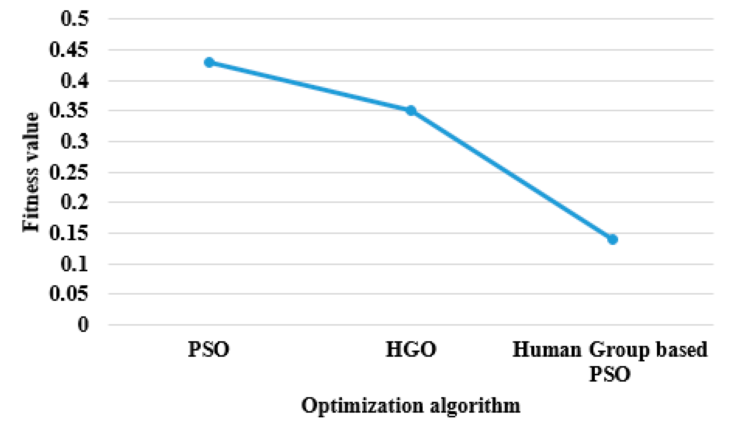
Compared to individual HGO and PSO algorithms, the proposed human group-based PSO algorithm has a minimum fitness value to select optimal feature vectors. The best fitness values of HGO, PSO and human group-based PSO algorithms is graphically represented in Figure 4.

3.4.2. Adaptive Uniform Mutation

The adaptive uniform mutation is utilized to increase the ability of the feature selection algorithm in exploration. In this operator, a non-linear function $p_m$ is used to control the range and decision of the mutation on each particle $p_i$. At every iteration, $p_m$ is updated using the Equation (14).

$$p_m=0.5\times e^{\left(-10\times \frac{n}{N}\right)}+0$$

(14)

where, $N$ is indicated as maximum iteration, $n$ denotes the number of iterations and the $p_m$ value tends to decrease when the number of iterations increases. The mutation randomly picks the $k$ elements from the particle, if the $p_m$ value is higher than the random number between [0, 1]. Then, the mutation value of the elements within the search space is reinitialized, where $k$ is an integer value, used for controlling the mutation range [61,62]. Mathematically, $k$ value is represented in Equation (15), as:

$$k=\max \left\{1,\hspace{0.17em}\left|D\times p_m\right|\right\}$$

(15)

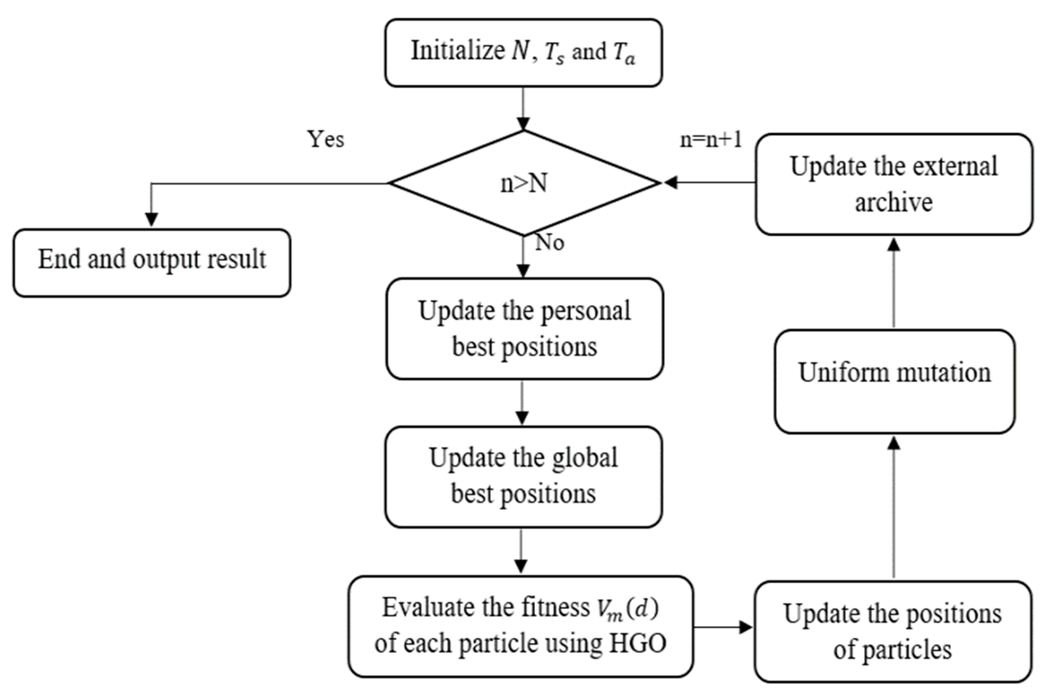
The flow chart related to the human group-based PSO algorithm is given in Figure 5, with the further description of the steps below.

The step by step process of human group-based PSO algorithm is given below.

Step 1: Initialize the particles swarm, (a) set the number of iterations $N$, swarm size $T_s$ and archive size $T_a$ (b) initialize the particles location, (c) estimate the objective of every particles, (d) save non-dominated solution into the archive.

Step 2: Pareto domination relationship is used to update the personal best position of the particles. If new position $p_i\left(n+1\right)$ is better than old personal best position $l{b}_i\left(n\right),\hspace{0.17em}set\hspace{0.17em}l{b}_i\left(n+1\right)=p_i(n+1)$, or else unchanged the personal best position of the particles, where $b_i$ is represented as best position and $l{b}_i(n)$ is presented as local best position.

Step 3: Based on the diversity of solution, select the global best position from the archive. At first, crowding distance value is calculated and then binary tournament is used to select the global best position of the particle $g{b}_i\left(n\right)$.

Step 4: Then, initialize the decision value $d_i$ based on $g{b}_i\left(n\right)$. Every decision $d_i$ of the feature vector $d$ is a binary value $d_i=\pm 1,\hspace{0.17em}i=1,2,\dots T$, every feature vector $d$ is related to the fitness value $V\left(d\right)$ that is considered as the weighted sum of $T$ stochastic contributions $W_j\left(d_j,d_1^j,..,d_s^j\right)$. However, these contributions depend on the value of decision $d_j$ and other $S$ decisions $d_i^j,i=1,2\dots S$.

The fitness function is mathematically presented in Equation (16):

$$V\left(d\right)=\frac{1}{T}{\displaystyle \sum _{j=1}^T{W}_j}\left(d_j,d_1^j,d_2^j,\dots ,d_s^j\right)$$

(16)

where the integer index $S=0,1,2,\dots T-1$ corresponds to the number of interacting decision values. The knowledge level of the $m^{th}$$m^{th}$ member is determined by the parameter $P\in \left[0,1\right]$, which is the probability of each member that knows the contribution of the decision. Based on the knowledge level, every member $m$ computes own perceived fitness using Equation (17):

$$V_m\left(d\right)=\frac{{\sum }_{j=1}^T{\stackrel{⌣}{d}}_{mj}{W}_j\left(d_j,d_1^j,d_2^j,\dots ,d_S^j\right)}{{\displaystyle \sum _{j=1}^T{\stackrel{⌣}{d}}_{mj}}}$$

(17)

where, $\stackrel{⌣}{d}$ is denoted as the matrix, whose generic element ${\stackrel{⌣}{d}}_{mj}$ considers the value one with probability $(P\hspace{0.17em}and\hspace{0.17em}0)$ with probability ($1-P$).

Step 5: Based on the decision value $d_i$, Equation (18) is used to update the velocity $v_i$ and position $p_i$ of the particles.

$$\begin{gathered} v_i\left(n+1\right)=w\times v_i\left(n\right)+r_1\times V_m\left(d\right)\times \left(l{b}_i\left(n\right)-p_i(n)\right)+r_2\times V_m(d)\times g{b}_i(n)-p_i\left(n\right)) \\ {p}_i(n+1)=p_i(n)+v_i(n+1) \end{gathered}$$

(18)

Step 6: Perform uniform mutation using the Equations (14) and (15).

Step 7: Update the external archive using crowding distance methodology.

Step 8: Analyze the termination condition: if the proposed algorithm attains the maximum iteration, then stop the algorithm, or else return to step 2. Hence, the worst particles (feature vectors) are eliminated based on the fitness function $V_m(d)$ of the HGO algorithm.

In all three datasets, approximately 70−80% of the feature vectors are selected from the total extracted features with this procedure. After selecting the optimal features, classification is then carried out using the LSTM classifier.

Table 3. Selected feature vectors after applying the feature selection algorithm.

Datasets	Extracted Features	Selected Features
Sat 4	$38\times 5000$	$38\times 3671$
Sat 6	$50\times 8700$	$50\times 6290$
Eurosat	$55\times 9000$	$55\times 7098$

states the extracted and the selected features after applying the human group-based PSO algorithm.

3.5. Classification

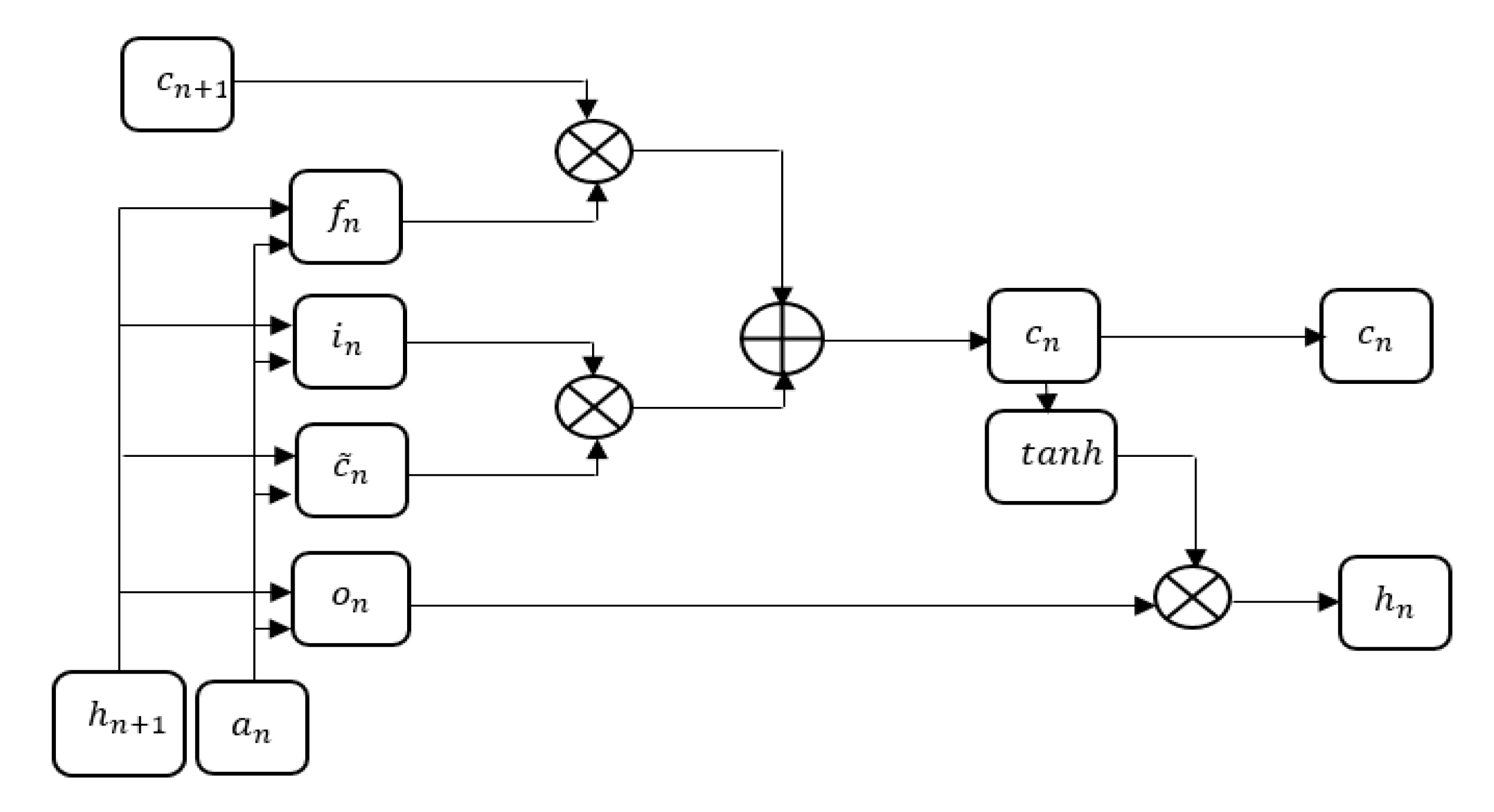
The LSTM classifier has the default behavior of remembering data information for a long period [63,64]. In a LULC classification, a huge number of remote sensing images are needed when neural networks are employed for attaining better results. Among different neural networks, the LSTM classifier has already proven to be the best choice in this case [65,66]. Generally, the LSTM classifier is composed of a series of LSTM units, where the temporal quasi-periodic features for extracting the long-term and short-term dependencies are stored. The structure of the LSTM classifier is denoted in Figure 6, and in our case, it includes 98 LSTM units, whose details are graphically stated in Figure 7.

Each single LSTM unit contains an input gate $i_n$, a forget gate $f_n$, a cell $c_n$ and an output gate $o_n$ which are mathematically expressed through the Equations (19)–(22):

$$i_n=\sigma \left(W_{ih}{h}_{n-1}+W_{ia}{a}_t+b_i\right)$$

(19)

$$f_n=\sigma \left(W_{fh}{h}_{n-1}+W_{fa}{a}_t+b_f\right)$$

(20)

$$c_n=f_n\times c_{n-1}+i_n\times \tanh (W_{ch}{h}_{n-1}+W_{ca}{a}_n+b_c)$$

(21)

$$o_n=\sigma \left(W_{oh}{h}_{n-1}+W_{oa}{a}_n+b_0\right)$$

(22)

where, represents the quasi-periodic feature in different frequency bands at the n time step. The output of the prior LSTM unit is stated as $h_{n-1}$.

Work coefficients are denoted as $W\hspace{0.17em}\mathrm{and}\hspace{0.17em}b$, while $\tanh (.)\hspace{0.17em}\mathrm{and}\hspace{0.17em}\sigma \left(.\right)$ indicate the hyperbolic tangent and sigmoid activation functions, respectively. The output of the LSTM unit is mathematically denoted in the following Equation (23):

$$h_n=o_n\times \tanh (c_n)$$

(23)

The output of the LSM unit at the n time step, $h_n$ contains the information of the prior time steps through $c_n\hspace{0.17em}\mathrm{and}\hspace{0.17em}{o}_n$, and collects the extracted features. Based on dependency relation, the cell state $\left\{c_n|n=1,2,,N\right\}$ learns the memory information of the temporal quasi-periodic features for a long and short period during the training process.

It is worth commenting, before moving to the next section, on one main issue of neural networks, which is represented by the overfitting that is the ability of fitting the training data, but not the testing data, because the network has not learned to generalize to new situations. The neural network is unable to exert its potential when in an overfitting state, and this may apply to the LSTM case. Early stopping operation with dropout and a weight constraint is one of the solutions utilized to train the neural networks and prevent gradient explosion and disappearance. Dropout randomly selects some LSTM units to set their output to zero during every iteration. The output value of a few LSTM units is used when calculating the error value; instead, some of the other LSTM units are discarded, and used only when error back propagation calculations must be performed. A LSTM network is trained by combining dropout with the constraining of the network parameters in order to suppress the overfitting [67], and a reasonable value for the hyper-parameters in the case of the LSTM employment are the following: 100 maximum epochs, 27 as minimum batch size, gradient threshold equals to 1, learning rate: 0.001, and layer wise hidden units respectively: layer 1: 200 units, layer 2: 225 units, layer 3: 200 units, and layer 4: 225 units. Further details can be found in [68].

4. Result and Discussion

The proposed model is simulated using the MATLAB 2019 version on a PC with 128 GB RAM, i9 Intel core processor, Windows 10 operating system (64-bit) and 3 TB hard disk. The performance of the proposed model is compared with a few benchmark models: GoogleNet [26], 2 band VGG [27], hyper parameter tuned VGG [27], 2 band AlexNet [27], hyper parameter tuned AlexNet [27], 2 band ConvNet [27], hyper parameter tuned ConvNet [27], AlexNet [28], ConvNet [28] and VGG [28], in order to find out its effectiveness. Specifically, the performance of the proposed model is evaluated on the selected datasets in terms of precision, recall and accuracy parameters. The mathematical expressions of accuracy, recall and precision are represented in the following Equations (24)–(26).

$$Accuracy=\frac{TP+TN}{FN+TP+TN+FP}\times 100$$

(24)

$$Recall=\frac{TP}{TP+FN}\times 100$$

(25)

$$Precision=\frac{TP}{TP+FP}\times 100$$

(26)

where, true negative is denoted as $TN$, false negative is represented as $FN$, true positive as $TP$ and false positive as $FP$.

In the following subsections, the quantitative evaluation of the proposed model is carried out when Sat 4, Sat 6 and Eurosat data are used. As a benchmark, the results presented in [26,27,28] works are considered.

4.1. Quantitative Investigation on Sat 4 Dataset

The Sat 4 dataset is used to evaluate the performance of the proposed model to classify four land-cover classes: tree, barren land, grassland and a class with all the other land covers. In this case, the performance evaluation is validated by using 500,000 image patches with 70% of the data used for training and 30% for testing.

Table 4. Performance investigation of the proposed model with different classifiers on Sat 4 dataset by means of recall and precision.

Classes	Human Group-Based PSO with DNN		Human Group-Based PSO with MSVM		Human Group Based-PSO with LSTM
	Precision (%)	Recall (%)	Precision (%)	Recall (%)	Precision (%)	Recall (%)
Barren land	99.07	99.12	99.65	99.79	99.90	99.98
Trees	99.54	99.65	99.67	99.65	99.98	99.97
Grasslands	99.60	99.87	99.43	99.80	99.97	99.95
Others	99.61	99.90	99.60	99.87	99.98	99.97
Overall	99.45	99.63	99.58	99.77	99.95	99.96

and

Table 5. Performance investigation of the proposed model with different classifiers on Sat 4 dataset by means of accuracy.

Classification Accuracy (%)
Classes	Human Group based PSO with DNN	Human Group Based PSO with MSVM	Human Group Based PSO with LSTM
Barren land	98.90	99.19	100
Trees	99.57	98.64	99.98
Grasslands	98.80	98.80	99.99
Others	99.15	98.76	100
Overall	99.10	98.84	99.99

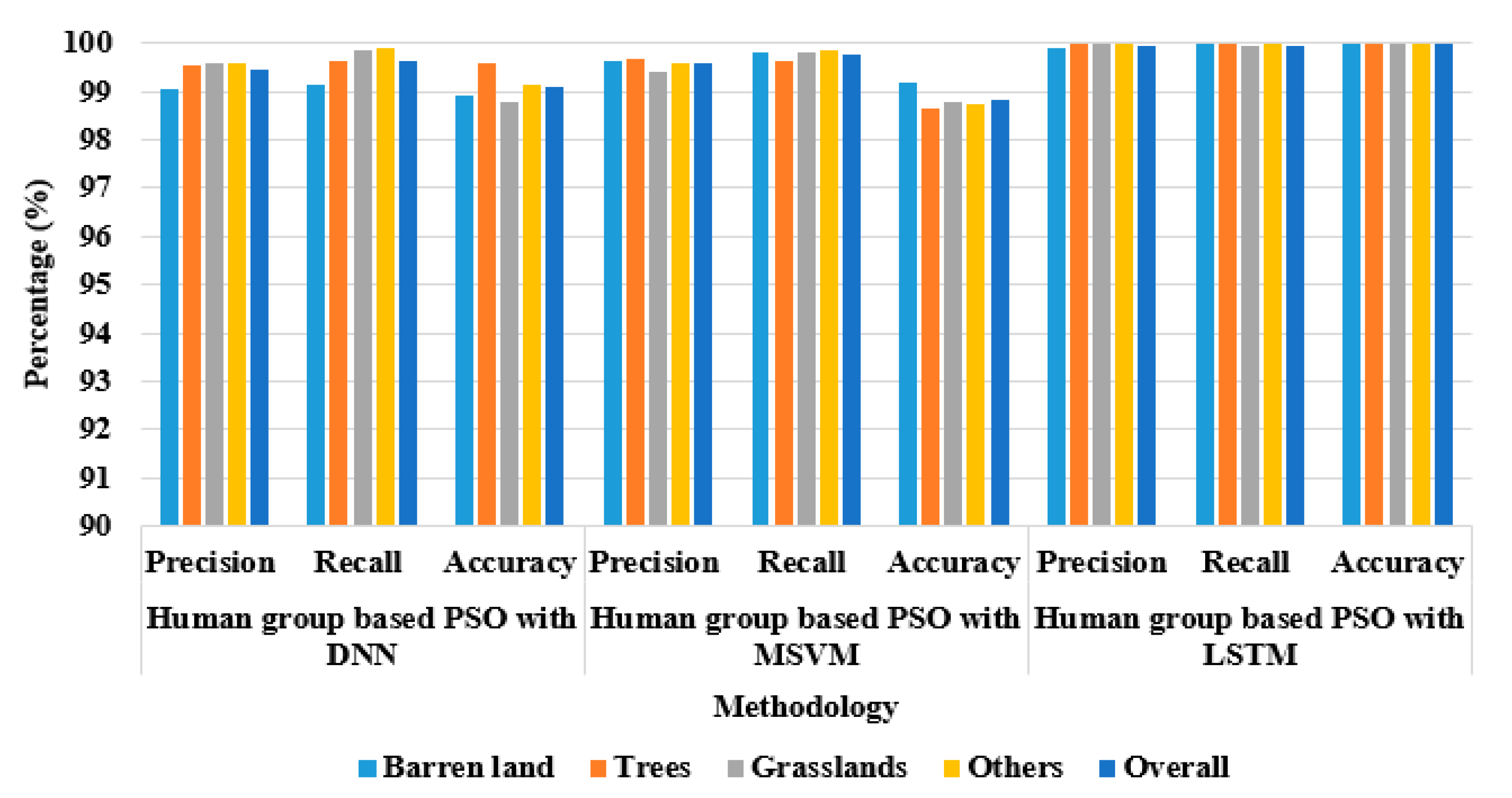
represent the performance evaluation of the proposed model, implementing an LSTM classifier, when the human group-based PSO is used with two other different classifiers, the Deep Neural Network (DNN) and the Multi Support Vector Machine (MSVM), in terms of recall and precision (Table 4), and in terms of accuracy (Table 5). The two tables point out that the LSTM classifier achieves better classification performance in LULC classification.

The same performance analysis of the proposed model with different classifiers on Sat 4 dataset is graphically represented in Figure 8.

Table 6. Performance investigation of the proposed model with different optimization techniques on Sat 4 dataset by means of recall and precision.

Classes	LSTM		PSO with LSTM		HGO with LSTM		Human Group Based PSO with LSTM
	Precision (%)	Recall (%)	Precision (%)	Recall (%)	Precision (%)	Recall (%)	Precision (%)	Recall (%)
Barren land	94.65	94.92	98.74	98.16	98.62	98.70	99.90	99.98
Trees	93	95	96.56	97.55	98.69	98.73	99.98	99.97
Grasslands	94.90	96.10	97.88	97.82	98.93	98.98	99.97	99.95
Others	93.70	94	98.63	98.87	98.69	98.92	99.98	99.97
Overall	94.06	95.005	97.95	98.10	98.65	98.83	99.95	99.96

and

Table 7. Performance investigation of the proposed model with different optimization techniques on Sat 4 dataset by means of classification accuracy.

Classification Accuracy (%)
Classes	LSTM	PSO with LSTM	HGO with LSTM	Human Group Based PSO with LSTM
Barren land	94.50	96.92	97.80	100
Trees	93	97.84	98.74	99.98
Grasslands	94.44	95.89	97.90	99.99
Others	93.92	97.78	98.89	100
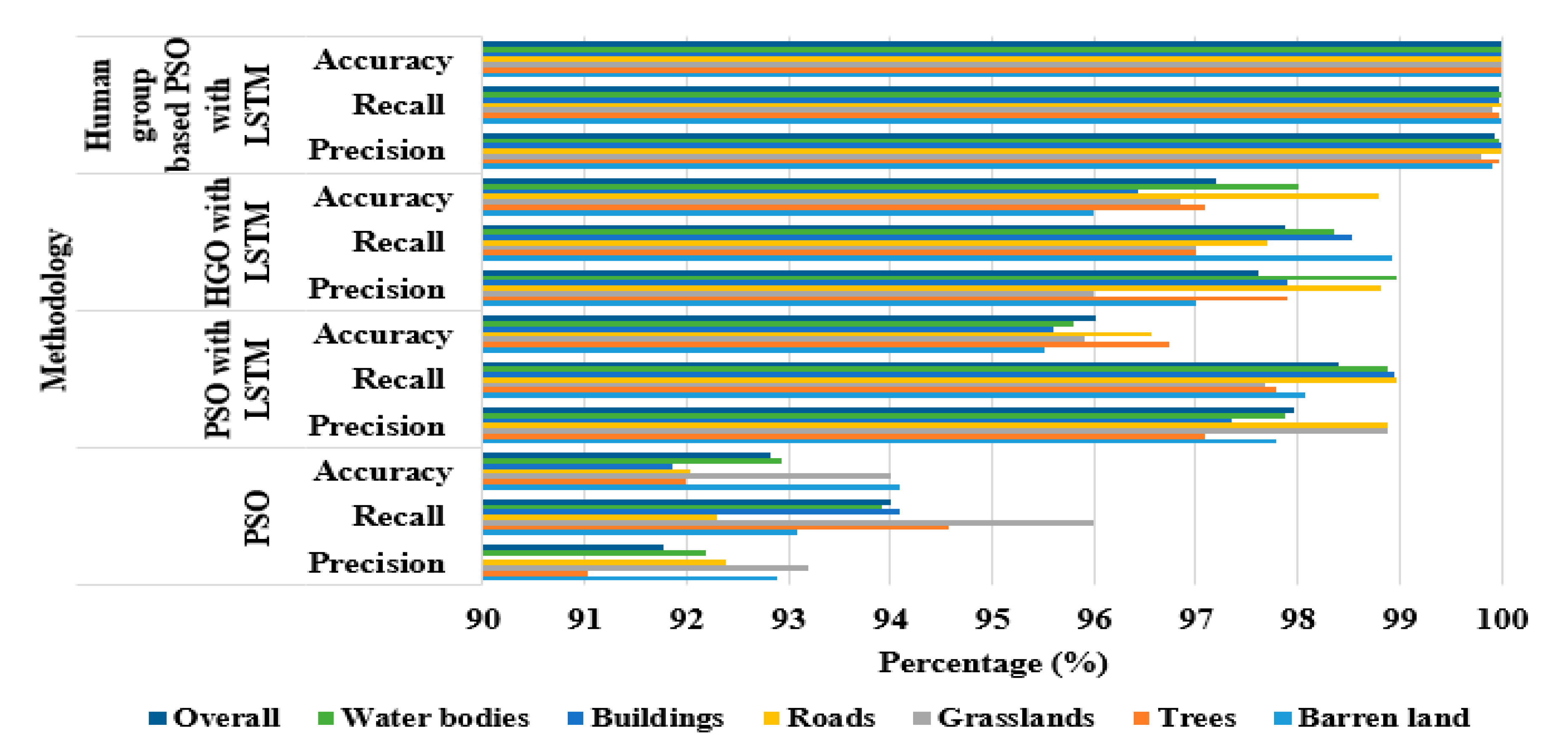
Overall	93.965	97.10	98.33	99.99

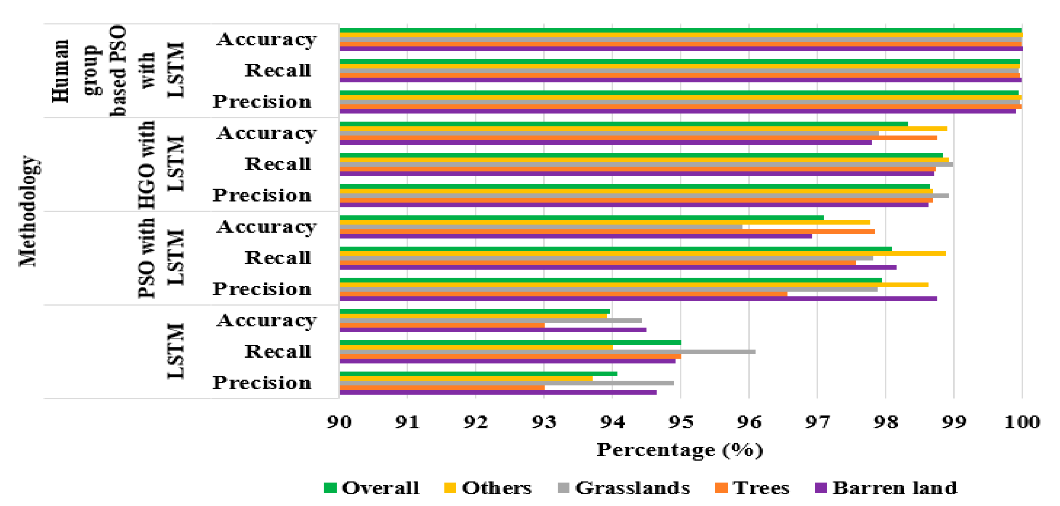
represent the performance evaluation of the proposed model when compared with other optimization techniques, like the LSTM only, the PSO with LSTM, the HGO with LSTM, and the human group-based PSO with LSTM, by means of recall and precision (Table 6) and by means of accuracy (Table 7). These tables are pointing out that the LSTM classifier with human group-based PSO achieves better performance in LULC classification in terms of recall, precision, and accuracy on the Sat 4 classes, as previously specified. The proposed model, the human group-based PSO with LSTM, shows a maximum of 6.03% improvement in LULC classification, if compared to LSTM, PSO with LSTM and Human Group Optimization (HGO) with LSTM. Figure 9 shows graphically the same performance analysis.

Comparison of Proposed Method with Existing Techniques on Sat 4 Dataset

In this subsection, AlexNet, ConvNet, and VGG [27] are selected for implementing the PSO and HGO techniques. The reason for choosing these techniques is that they are the most widely used neural network architectures for the classification of LULC on satellite images. The selected existing techniques are implemented with HGO and PSO after the max pooling layer of each existing technique. For instance, ConvNet has the output of 4.096 features in the max pooling layer and implemented the PSO and HGO as filtering technique that provides only 1000 features as output of fully ConvNet.

Table 8. Comparative analysis of different neural networks with PSO and HGO.

Methodology	Dataset	Overall Accuracy (%)
AlexNet + PSO	Sat 4	99.95 ± 0.02
AlexNet + HGO	Sat 4	99.94 ± 0.02
AlexNet + PSO + HGO	Sat 4	99.96 ± 0.02
ConvNet + PSO	Sat 4	99.94 ± 0.02
ConvNet + HGO	Sat 4	99.95 ± 0.01
ConvNet + PSO + HGO	Sat 4	99.96 ± 0.02
VGGNet + PSO	Sat 4	99.95 ± 0.03
VGGNet + HGO	Sat 4	99.95 ± 0.03
VGGNet + PSO + HGO	Sat 4	99.96 ± 0.02
Proposed LSTM + PSO	Sat 4	99.97 ± 0.02
Proposed LSTM + HGO	Sat 4	99.97 ± 0.02
Proposed LSTM+ PSO + HGO	Sat 4	99.98 ± 0.01

shows the performance evaluation of the proposed model when compared with these various neural networks on Sat 4 dataset, in terms of classification accuracy. From the analysis, the results confirm that the proposed LSTM with PSO and HGO achieved better performance on LULC classification in terms of accuracy on Sat 4 dataset.

Sample image patches of Sat 4 dataset for the selected classes are given in Figure 10.

It is worth to underline that the size of each image patch in Sat 4 dataset is $28\times 28$ m, quite small, and this limits the possibility to enlarge the image since it appears very unfocused.

4.2. Quantitative Investigation on Sat 6 Dataset

The same analysis carried out in the previous Section 4.1 on Sat 4 is now assessed on Sat 6 dataset. In this case, the dataset is used to evaluate the performance of the proposed model to classify six land cover classes: grassland, water bodies, buildings, barren land, roads and trees. The performance analysis is carried out by using 40.500 image patches with 70% of them for training and 30% for testing. The performance of the proposed model is analyzed with different classification techniques, DNN, MSVM, LSTM (

Table 9. Performance investigation of the proposed model with different classifiers on Sat 6 dataset by means of recall and precision.

Classes	Human Group Based PSO with DNN		Human Group Based PSO with MSVM		Human Group Based PSO with LSTM
	Precision (%)	Recall (%)	Precision (%)	Recall (%)	Precision (%)	Recall (%)
Barren land	98.97	99.02	96.09	99.07	99.92	99.99
Trees	99	98.76	99	98.90	99.98	99.98
Grasslands	99.82	99.05	98.45	99.09	99.80	99.90
Roads	99.80	98.90	99.12	98.85	100	100
Buildings	99.30	97.98	98.80	98.98	100	99.98
Water bodies	99.87	99	99	99.80	99.98	100
Overall	99.46	98.785	98.41	99.115	99.94	99.975

and

Table 10. Performance investigation of the proposed model with different classifiers on Sat 6 dataset by means of classification accuracy.

Classification Accuracy (%)
Classes	Human Group Based PSO with DNN	Human Group Based PSO with MSVM	Human Group Based PSO with LSTM
Barren land	98.90	99	100
Trees	98.72	98.96	99.99
Grasslands	99.09	96.09	99.99
Roads	98.79	95.97	100
Buildings	98.90	98.06	99.99
Water bodies	99	99.5	100
Overall	98.90	97.88	99.99

), and with different optimization techniques, LSTM only, the PSO with LSTM, the HGO with LSTM, and the human group-based PSO with LSTM (

Table 11. Performance investigation of the proposed model with different optimization techniques on Sat 6 dataset by means of recall and precision.

Classes	LSTM		PSO with LSTM		HGO with LSTM		Human Group Based PSO with LSTM
	Precision (%)	Recall (%)	Precision (%)	Recall (%)	Precision (%)	Recall (%)	Precision (%)	Recall (%)
Barren land	92.90	93.09	97.78	98.08	97	98.92	99.92	99.99
Trees	91.02	94.57	97.09	97.79	97.89	97	99.98	99.98
Grasslands	93.20	96	98.88	97.68	96	97	99.80	99.90
Roads	92.39	92.30	98.89	98.97	98.82	97.71	100	100
Buildings	89	94.09	97.35	98.95	97.90	98.54	100	99.98
Water bodies	92.19	93.92	97.88	98.89	98.96	98.35	99.98	100
Overall	91.78	93.995	97.97	98.39	97.61	97.87	99.94	99.975

and

Table 12. Performance investigation of the proposed model with different optimization techniques on Sat 6 dataset by means of classification accuracy.

Classification Accuracy (%)
Classes	LSTM	PSO with LSTM	HGO with LSTM	Human Group Based PSO with LSTM
Barren land	94.09	95.52	96	100
Trees	92	96.73	97.08	99.99
Grasslands	94	95.90	96.85	99.99
Roads	92.03	96.57	98.80	100
Buildings	91.86	95.60	96.43	99.99
Water bodies	92.94	95.80	98	100
Overall	92.82	96.02	97.19	99.99

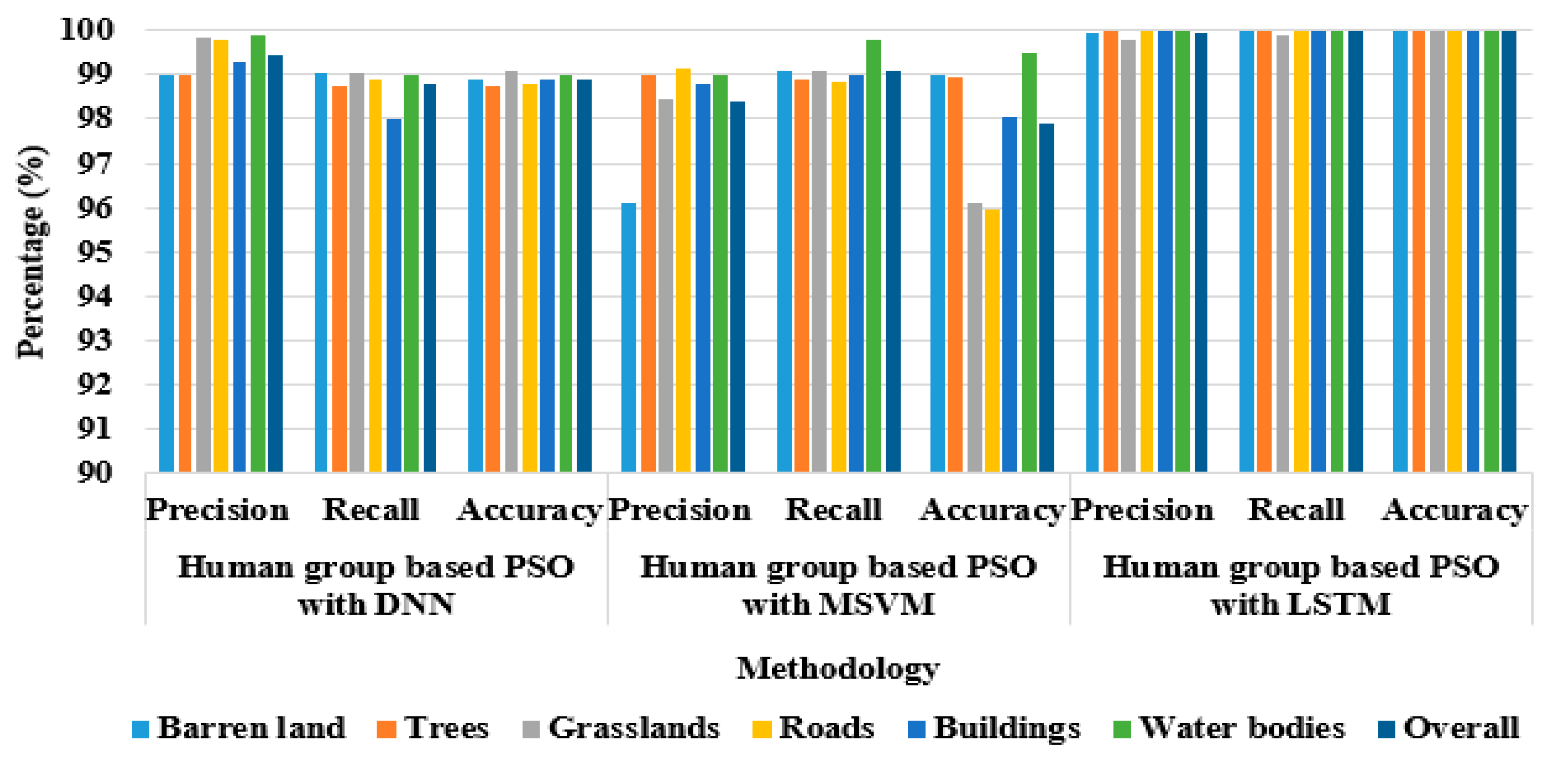
), by means of recall and precision (Table 9 and Table 11) and by means of accuracy (Table 10 and Table 12). The results summarized in the following Table 9 and Table 10, respectively, point out how the LSTM classifier achieves better performance in LULC classification, if compared to other classification techniques, also in this case, when Sat 6 dataset is used. Performance analysis of the proposed model with different classifiers on Sat 6 dataset is also graphically presented in Figure 11.

The results summarized in the following Table 11 and Table 12, respectively, point out how the proposed model achieves better performance in LULC classification, if compared to other different optimization techniques on Sat 6 dataset. The Tables show how the proposed model, the human group-based PSO with LSTM, reaches a maximum of 7.17% and minimum of 2.8% improvement in LULC classification compared to the only LSTM, to the PSO with LSTM and to the HGO with LSTM.

Performance analysis of the proposed model with different optimization techniques on Sat 6 dataset is also graphically presented in Figure 12.

Comparison for the Proposed LSTM Method with Existing Techniques on Sat 6 Dataset

In this subsection, LSTM, AlexNet, VGG and ConvNet are implemented with PSO and HGO on the Sat 6 dataset. Eight layers are presented in the AlexNet, where the first five layers are convolution layers followed by max-pooling layers and the remaining three are fully connected layers. The second fully connected layer produces as output 4096 features. Here, the PSO and HGO are implemented to minimize the features. Therefore, the final output of AlexNet is 1.000 features. Likewise, the other neural networks are implemented with PSO and HGO after the max-pooling layers.

Table 13. Comparative analysis of proposed LSTM with existing neural networks on Sat 6 dataset.

Methodology	Dataset	Overall Accuracy (%)
AlexNet + PSO	Sat 6	99.88 ± 0.03
AlexNet + HGO	Sat 6	99.89 ± 0.02
AlexNet + PSO + HGO	Sat 6	99.91 ± 0.01
ConvNet + PSO	Sat 6	99.86 ± 0.03
ConvNet + HGO	Sat 6	99.88 ± 0.02
ConvNet + PSO + HGO	Sat 6	99.90 ± 0.01
VGGNet + PSO	Sat 6	99.92 ± 0.02
VGGNet + HGO	Sat 6	99.92 ± 0.02
VGGNet + PSO + HGO	Sat 6	99.93 ± 0.01
Proposed LSTM + PSO	Sat 6	99.98 ± 0.02
Proposed LSTM + HGO	Sat 6	99.98 ± 0.02
Proposed LSTM+ PSO + HGO	Sat 6	99.98 ± 0.01

describes the comparison of the proposed model with the different neural networks, AlexNet, VGGNet and ConvNet with PSO and HGO, on the whole Sat 6 dataset in terms of overall classification accuracy. In this case, LSTM + PSO + HGO attain 99.94% of precision, 99.97% of recall and 99.99% of accuracy. Sample image patches of the Sat 6 dataset for the selected classes are given in Figure 13. The size of each patch is $28\times 28$ m also in the case of the Sat 6 dataset, and the same issue already discussed is faced when images of the patches are shown.

4.3. Quantitative Investigation on Eurosat Dataset

In this section, Eurosat dataset is used to evaluate the performance of the proposed model to classify 12 LULC classes. Those are permanent crop, annual crop, pastures, river, sea and lake, forest, herbaceous vegetation, industrial building, highway and residential building. In this scenario, the performance analysis is accomplished for 27,000 image patches with 70% of the data used for training and 30% for testing with two case studies.

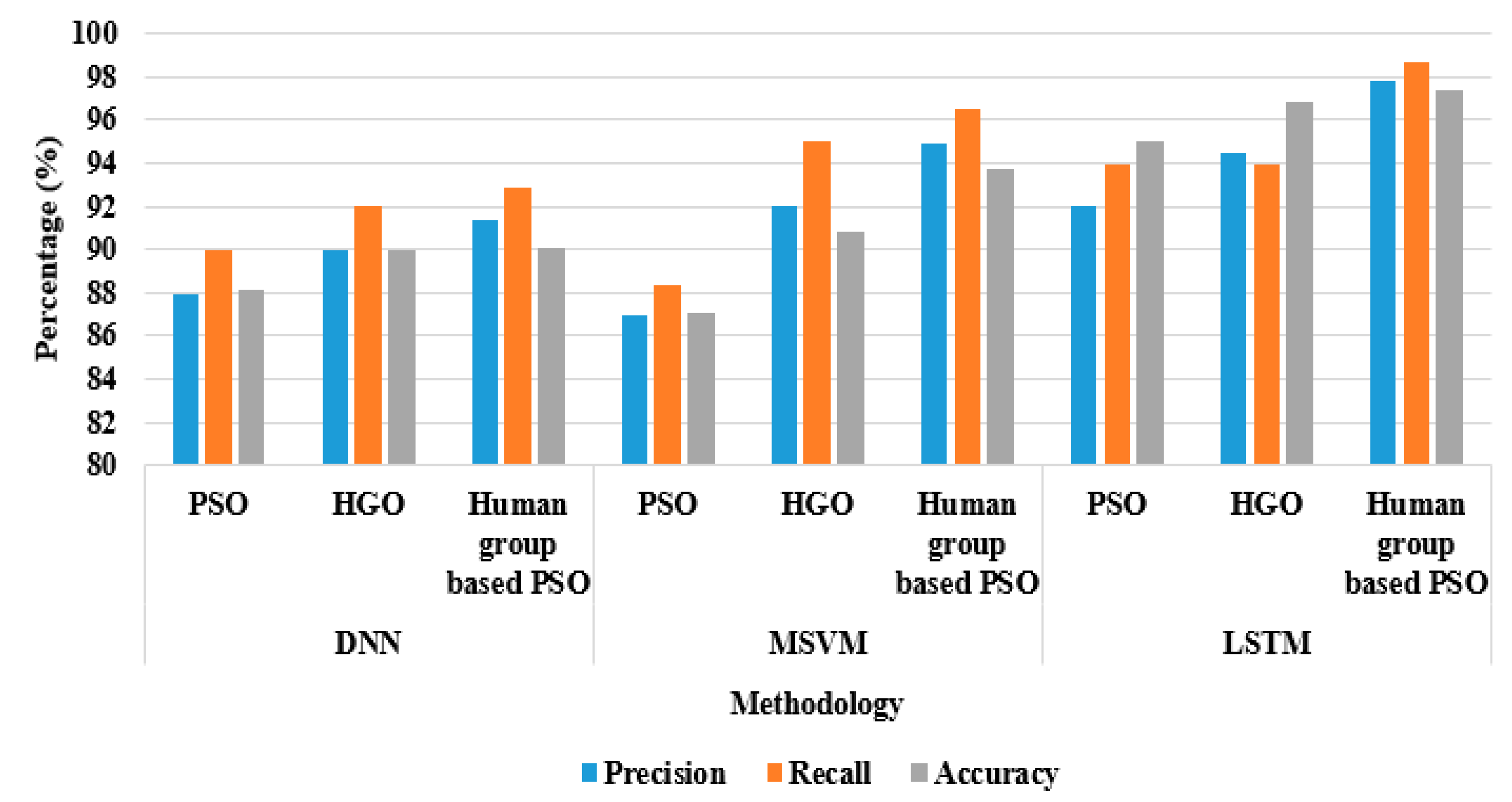
In this case,

Table 14. Performance investigation of the proposed model on Eurosat dataset.

Average Value
Classification	Optimization Techniques	Precision (%)	Recall (%)	Accuracy (%)
DNN	PSO	87.89	90	88.2
	HGO	90	92.02	90
	HGO + PSO	91.38	92.91	90.09
MSVM	PSO	87	88.39	87.03
	HGO	92.04	95	90.85
	HGO + PSO	94.90	96.50	93.70
LSTM	PSO	92	93.98	95
	HGO	94.50	94	96.90
	HGO + PSO	97.80	98.70	97.40

summarizes the performance values of the proposed model for different classes of LULC classification in terms of accuracy, recall and precision, with different classifiers, DNN, MSVM, LSTM, and different optimization techniques, PSO, HGO and human group-based PSO. The accuracy, recall and precision of the LSTM classifier with human group-based PSO is 97.40%, 98.70% and 97.80%, respectively. The LSTM classifier with human group-based PSO shows an improvement in LULC classification also in this case, when tested on the Eurosat dataset. Performance analysis of the proposed model on Eurosat dataset is graphically presented in Figure 14.

Comparison of Implementing PSO and Human Group Optimization (HGO) on the Proposed Method

In this subsection, GoogleNet [26] is implemented with optimization techniques, namely PSO and HGO, and only 1.000 features are selected. The other techniques like AlexNet, VGG, and ConvNet, as presented in [27], worked only on the Sat 4 and Sat 6 dataset, hence, they were not considered in the case study of the Eurosat dataset. The GoogleNet uses 1 × 1 convolutions in the middle of the architecture, and global average pooling. In addition, the inception module is also different from other architectures. The 1 × 1, 3 × 3, 5 × 5 convolutions are presented in the inception module and 3 × 3 max pooling is operated in a parallel way and the input and output are stacked together for generating the final output.

Table 15. Comparative analysis of proposed LSTM with PSO and HGO on the Eurosat dataset.

Methodology	Dataset	Overall Accuracy (%)
GoogleNet + PSO	Eurosat	96.18 ± 0.3
GoogleNet + HGO	Eurosat	96.20 ± 0.2
GoogleNet + PSO + HGO	Eurosat	96.40 ± 0.2
Proposed LSTM + PSO	Eurosat	97.37 ± 0.03
Proposed LSTM + HGO	Eurosat	97.39 ± 0.02
Proposed LSTM+ PSO + HGO	Eurosat	97.40 ± 0.01

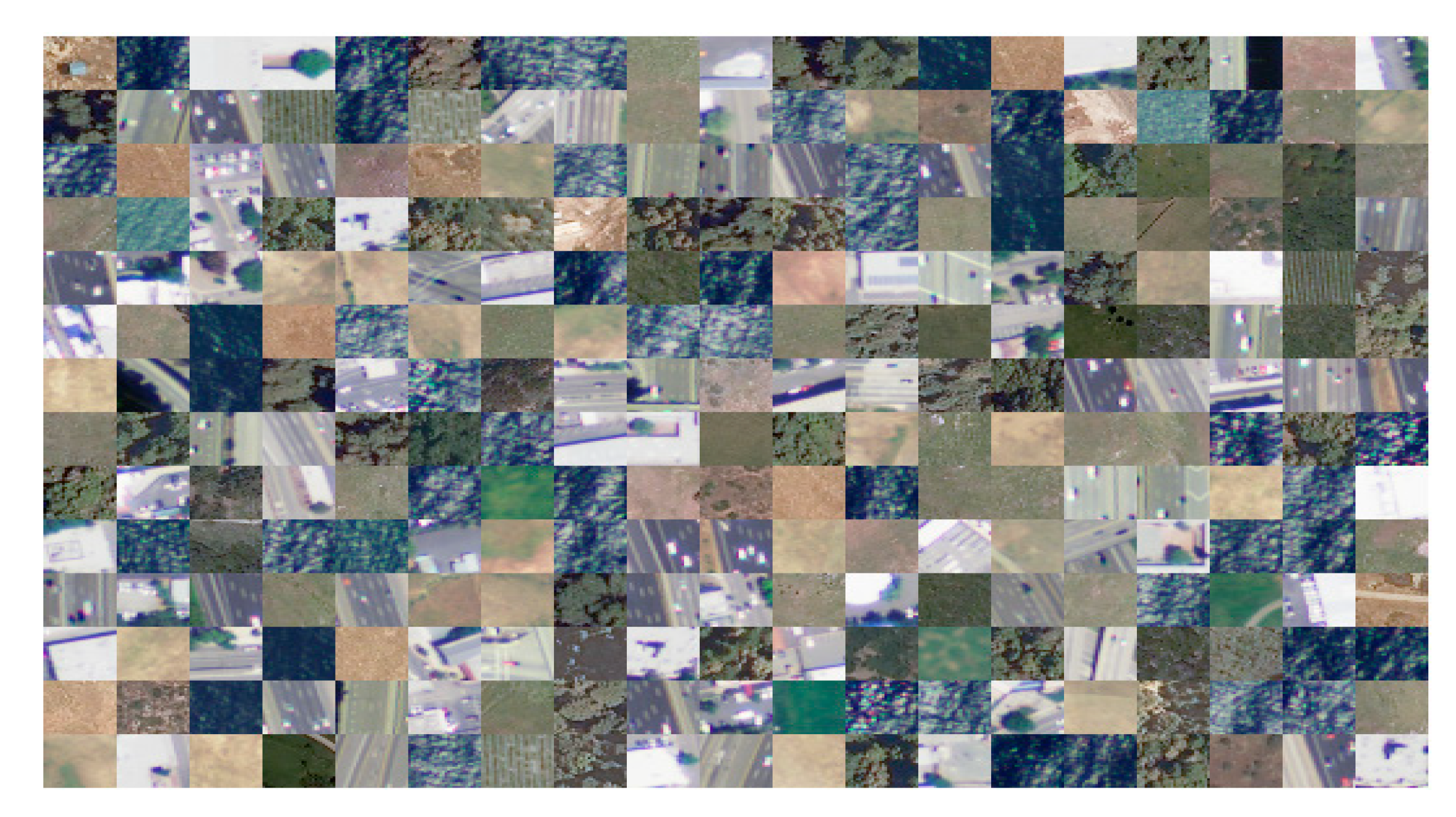
shows the comparative analysis of LSTM and GoogleNet [26] with PSO and HGO on the whole Eurosat dataset. Sample image patches of the Eurosat dataset are given in Figure 15. In this case, the image could be realized with a better focus, since the size of each patch is $64\times 64$ m.

4.4. Comparative Analysis

The comparative analysis between the proposed and existing models is represented in

Table 16. Comparative investigation of the proposed and existing models.

Methodology	Dataset	Overall Accuracy (%)
GoogleNet [26]	Eurosat	96.69
2 band AlexNet [27]	Sat 4	99.66
	Sat 6	99.08
Hyper parameter tuned AlexNet [27]	Sat 4	98.45
	Sat 6	97.43
2 band ConvNet [27]	Sat 4	99.03
	Sat 6	99.10
Hyper parameter tuned ConvNet [27]	Sat 4	98.45
	Sat 6	97.48
2 band Visual Geometric Group (VGG) [27]	Sat 4	99.03
	Sat 6	99.15
Hyper parameter tuned VGG [27]	Sat 4	98.59
	Sat 6	97.95
AlexNet [28]	Sat 4	99.98
	Sat 6	99.93
AlexNet-small [28]	Sat 4	99.86
	Sat 6	99.90
VGG [28]	Sat 4	99.98
	Sat 6	99.98
Proposed model	Eurosat	97.40
	Sat 4	99.99
	Sat 6	99.99

. Analyzing recent works from the literature, based on similar data, it was found that Helber et al. [26] developed a new patch-based LULC classification technique using Eurosat dataset. As already discussed, this work explained how CNN was used to detect the LULC changes, by helping to improve the geographical maps. Unnikrishnan et al. [27] implemented a novel deep learning method for three different networks VGG, AlexNet and ConvNet, and Sat 4 and Sat 6 datasets were used to analyze the performance of the developed model. Papadomanolaki et al. [28] designed a deep learning model based on a CNN for accurate land-cover classification, by including 2 band information (red and near infrared) with a reduced number of filters, which were tested and trained to classify the images into different classes. In our manuscript, the proposed architecture was directly compared with these models in terms of precision, recall and accuracy.

Table 16 illustrates that the proposed model achieves a minimum of 0.01% and a maximum of 2.56% improvement in accuracy on Sat 4, Sat 6 and Eurosat datasets, when compared with the models presented in [26,27,28]. The improvement is there, although modest, but it is worth adding also that the human group-based PSO algorithm, presented in this work, when combined with a LSTM classifier gains a better performance in LULC classification also by means of computational cost and processing time. Compared to DNN and MSVM, LSTM has less training time for all three datasets. Moreover, the proposed human group-based PSO algorithm significantly reduces the “curse of dimensionality” problem and the LSTM classifier achieves better performance in LULC classification, as demonstrated before, when compared with other classifiers. This better LULC classification may assist the researchers in many real time applications such as wildlife habitat protection, urban expansion/encroachment, natural resource management, legal boundaries for tax and property evaluation, target detection (identification of land/water interface, clearings, roads, bridges, and landing strips), damage delineation (flooding, seismic, tornadoes, volcanic, and fire), and routing/logistics planning for resource extraction activities, exploration and seismic.

4.5. Final Discussion

As highlighted in the methodology section, feature selection is an integral part of LULC classification in this research paper. Several feature vectors are extracted from the images using LGBPHS, HOG and Haralick approaches, and feature selection is used to choose optimal feature vectors for better classification. The effects of feature selection are shown in Table 6, Table 7, Table 11, and Table 12, where the experimental analysis is verified by determining the performance measures. Related to individual LSTM, PSO with LSTM, and HGO with LSTM, the proposed human group-based PSO with LSTM showed a maximum of 6.03% and a minimum of 1.66% improvement in LULC classification on Sat 4 dataset. Similarly, the proposed human group-based PSO with LSTM showed a maximum of 7.17% and minimum of 2.80% improvement in LULC classification on the Sat 6 dataset. In addition to this, the proposed human group-based PSO with LSTM achieved a minimum of 0.01% and a maximum of 2.56% improvement in classification accuracy on Sat 4, Sat 6 and Eurosat datasets compared to the existing methodologies like GoogleNet [26], 2 band AlexNet [27], Hyper parameter tuned AlexNet [27], 2 band ConvNet [27], Hyper parameter tuned ConvNet [27], 2 band VGG [27], Hyper parameter tuned VGG [27], AlexNet [28], AlexNet-small [28], and VGG [28]. It has been also highlighted how the proposed model presents a better performance in LULC classification even by means of computational cost and processing time.

In this work, experimental analysis was focused on differentiating the things that are not related to human habitats, in both urban and agricultural environments. Future work will extend the proposed analysis to other applications, including human habitats.

5. Conclusions

The objective of this study was to propose an effective feature selection model to classify the LULC classes of the urban and agricultural environment. The proposed model helped to analyze the changes in land productivity, soil quality, and biodiversity, for instance, which provided a clear idea about environmental quality, wildlife habitat, loss of prime agricultural lands, uncontrolled development, etc. In this study, an optimization procedure based on the combination of LGBPHS, HOG and Haralick texture features was first utilized to extract the feature vectors of the objects from the normalized remote-sensing images. The human group-based PSO algorithm was then applied to select the optimal feature vectors that helped in further improving the performance of classification. The optimal selected features were given as the input to an LSTM classifier. The proposed model achieved a better performance when compared to the existing models in LULC classification in terms of recall, accuracy and precision. The simulation results showed that the proposed model achieved enhancements in classification accuracy on the Sat 4, Sat 6 and Eurosat datasets. In addition, the computational time of the proposed model is only 1.24 s. The main findings of the human group-based PSO algorithm delivered up to date dynamics of LULC in the Sat 4, Sat 6 and Eurosat datasets. These datasets are used to monitor the future changes, LULC planning process and other similar studies in the European countries. In future work, an optimization based clustering approach will be included in the proposed model to verify if the LULC classification method can be further improved.