A Deep Learning Method for Mapping Glacial Lakes from the Combined Use of Synthetic-Aperture Radar and Optical Satellite Images

Abstract

Glacial lakes (GLs), a vital link between the hydrosphere and the cryosphere, participate in the local hydrological process, and their interannual dynamic evolution is an objective reflection and an indicator of regional climate change. The complex terrain and climatic conditions in mountainous areas where GLs are located make it difficult to employ conventional remote sensing observation means to obtain stable, accurate, and comprehensive observation data. In view of this situation, this study presents an algorithm with a high generalization ability established by optimizing and improving a deep learning (DL) semantic segmentation network model for extracting GL contours from combined synthetic-aperture radar (SAR) amplitude and multispectral imagery data. The aim is to use the high penetrability and all-weather advantages of SAR to reduce the effects of cloud cover as well as to integrate the multiscale and detail-oriented advantages of multispectral data to facilitate accurate, quantitative extraction of GL contours. The accuracy and reliability of the model and algorithm were examined by employing them to extract the contours of GLs in a large region of south-eastern Tibet from Landsat 8 optical remote sensing images and Sentinel-1A amplitude images. In this study, the contours of a total 8262 GLs in south-eastern Tibet were extracted. These GLs were distributed predominantly at altitudes of 4000–5500 m. Only 17.4% of these GLs were greater than 0.1 km² in size, while a large number of small GLs made up the majority. Through analysis and validation, the proposed method was found highly capable of distinguishing rivers and lakes and able to effectively reduce the misidentification and extraction of rivers. With the DL model based on combined optical and SAR images, the intersection-over-union (IoU) score increased by 0.0212 (to 0.6207) on the validation set and by 0.038 (to 0.6397) on the prediction set. These validation data sufficiently demonstrate the efficacy of the model and algorithm. The technical means employed in this study as well as the results and data obtained can provide a reference for research and application expansion in related fields.

1. Introduction

Mountainous glacial lakes (GLs) are a major constituent of lake groups and are vitally important for research relating to water resources, cryospheric science, climate, and mountain disasters [1,2]. In order to better understand water level changes, Wen et al. used the deep learning (DL) model to simulate and predict the lake level dynamics of Sumu Barun Jaran on a 2-h timescale [3]. The available data have shown increasing climate warming and glacial melting as well as a continuous increase in precipitation in West China in the past five decades [4]. This has affected the local meltwater effect [5], runoff, and hydrological processes [6] and accelerated the evolution of GLs and increased their outburst risk. Many scholars also expressed concern about the collapse of the ice lake: Richardson et al. researched glacier disasters in the Himalayas, with particular emphasis on glacial lake outburst disasters [7]. Extracting GL contours and monitoring changes in GL areas are crucial for GL outburst prevention and control and can provide decision-making support for secondary GL disaster prevention and control.

Obtaining GL boundary information has always been a difficult task in GL research. GLs are often located in remote, high-altitude areas, making manual field measurements difficult. As a result, remote sensing has become a core technology for monitoring GLs. The Landsat series of satellites has provided the longest surface observation times and spatial records. The Landsat 8 satellite, launched in 2013, covers a wide surface area and has a good signal-to-noise ratio. In addition, the Landsat 8 Level-1 terrain-corrected products generated based on ground control points can be directly used to classify surface features. Numerous experimental studies have demonstrated the reliability of data collected by the Landsat series of satellites for cryospheric science-related research [8,9,10]. Many researchers in China and elsewhere have extensively investigated effective methods for extracting GL contours from remote sensing images. Yang et al. visually interpreted GLs in West China on a large scale based on Landsat 8 data combined with the Google Earth software (Sourced from the USA) [11]. Zhang et al. manually vectorized GLs for three periods of time, namely, 1990, 2000, and 2010 [12]. Relatively good results have been achieved by employing spectral information index (e.g., the normalized difference water index (NDWI) and the modified NDWI (MNDWI)) threshold methods to extract the contours of bodies of water from multispectral remote sensing images [13,14]. However, it is difficult to distinguish bodies of water from land with single water indexes (WIs). The lake detection algorithm proposed by Bhardwaj [15] and the glacial lake inventory proposed by Wessels et al. [16] each combine thermal infrared and digital elevation model data and effectively improve the misclassification problem associated with single WIs by accounting for the difference in turbidity between GLs. Yang et al. combined WI and improved fuzzy clustering (termed WIMFCM) methods to mitigate the deficiencies of single WIs [9]. Some researchers have also extracted the contours of bodies of water based on morphological features combined with WIs. Chen et al. [17] and Barbieux et al. [18] used the NDWI in combination with the active contour method to extract GL contours. Luo et al. first approximately extracted the contours of bodies of water using the NDWI and subsequently refined the extracted contours using a distributed iterative method [19]. Synthetic-aperture radar (SAR) is able to penetrate clouds. Using SAR to study GLs is one of the current focal areas of research. Tom et al. monitored lake ice by analyzing Sentinel-1 data with deep learning (DL) [20]. Wen et al. examined dynamic changes in lake water levels using DL and multivariate linear regression techniques [3]. Zhang et al. analyzed the seasonal changes in large lakes on the Tibetan Plateau by analyzing Sentinel-1 data using a support vector machine [21]. Zhang et al. reported a time-series analysis of the changes in the GLs at the end of the Gongba Glacier in the period 2007–2018 based on the intensity standardization ratio of SAR images [22]. Hanshaw et al. used 158 multispectral satellite images spanning almost four decades, from 1975 to 2012, to obtain lake-area outlines for the understudied Cordillera Vilcanota region [23]. These methods facilitate the extraction of GL contours and increase the understanding of the temporal and spatial development of GLs. However, extensive manual interpretation and editing remain a factor that circumscribes the development of GL monitoring. The available extraction methods often target large lakes that are larger than a certain size threshold in local areas and require images without cloud cover. Multiscale, multiregional schemes for extracting GL contours are lacking.

GLs differ considerably from ordinary lakes. The identification of GLs is significantly affected by myriad factors, including intrinsic complex geomorphic features, fragmented spatial distribution patterns, varied water composition, differences in turbidity caused by the influx of glacial sediments from their sources, and changes in the overall spectral information from their waters caused by cloud cover, frozen surfaces, and shadows cast by mountains. As a consequence, it is difficult to apply traditional methods such as ratio method, index method, supervised classification and unsupervised classification to extract the contours of bodies of water from satellite remote sensing images of GL areas [15,17]. This study, for the first time, presents a DL method to extract GL contours from Landsat 8 and Sentinel-1 data. This method sufficiently accounts for the effects of GL diversity and interference factors (e.g., frozen lake surfaces as well as cloud cover). The main objectives of this study are to (1) examine the reliability of DL in extracting the contours of mountainous GLs in south-eastern Tibet and (2) to improve the robustness of GL contour extraction against interference by introducing SAR images.

2. Model and Algorithm

U-Net, a DL model [24], is a typical deep convolutional encoder. The U-Net architecture consists primarily of three parts, namely, encoding, decoding, and concatenation, and its shape is similar to that of the letter “U”, hence the name of the model (as shown in Figure 1). U-Net is established by restructuring and optimizing the architecture of fully convolutional networks to obtain a high-accuracy classification model with a relatively small amount of training data. U-Net is a relatively classical model for extracting information from objects in the image segmentation field. In recent years, a number of new U-Net-based algorithms have emerged, including U-Net++ [25] and Deeplabv3+ [26]. In the available models, depthwise separable or atrous convolutions are generally implemented to increase the model’s depth and, at the same time, reduce the number of parameters. However, GLs are small objects in images, and they are distributed in a dispersed pattern and differ in size. As a result, when used to extract GL contours, a U-Net-based model is prone to divergence and identification of positive sample data as the background, and the loss function is prone to tending to zero. This makes it difficult to ensure the accuracy of the result.

2.1. U-Net Model Architecture

In this study, the U-Net DL model is, for the first time, employed to extract GL contours from remote sensing images. In addition, it is proposed that SAR amplitude images be used as an adjunct to multispectral images to facilitate comprehensive extraction of GL contour features. To achieve this, the U-Net model is optimized and improved to be more applicable for the extraction of GL contours from multisource remote sensing images. Figure 1 shows the main structure of the improved U-Net model. Encoding is achieved primarily by maximum pooling. The shallow convolutional layer close to the input is used to extract small-scale, simple features. The receptive field of the model is improved by changing the image scale and increasing the number of image channels. This allows the deep convolutional layers to obtain multiscale, high-level semantic information about the image. Decoding is the opposite of encoding. The decoding procedure integrates a large number of high-dimensional features, reduces the dimensionality of the channels, and increases the image scale. Through the stacking of the decoding layers, the image is restored to its original size, and the corresponding predicted data are generated. There are a large number of functional channels between the encoder and decoder of this U-Net model. These channels connect the low- and high-layer information and, thereby, reduce the effects of the information losses that occur during downsampling on the result. Moreover, by integrating multiscale information, these channels accelerate the convergence of the model and improve its segmentation accuracy.

2.2. Principle and Algorithm Analysis

Remote sensing images contain complex information. The proportion of lake information in most image blocks is extremely small (generally < 2%). The cross-entropy error and the mean squared error, which are often used in DL, are inapplicable to data with extremely unbalanced positive and negative samples. Thus, in this study, the Tversky function is adopted as a loss function to balance positive and negative samples. The Tversky function was initially designed to address the imbalance between lesions and nonlesions encountered when classifying medical images using machine learning (ML). The recall metric is improved by balancing the proportions of false positives and false negatives in training. This facilitates a relatively good trade-off between accuracy and sensitivity in the function. Equation (1) is the Tversky function.

$$T(A,B)=\frac{|A\cap B|}{|A\cap B|+\alpha |A-B|+\beta |B-A|}$$

(1)

where $A$ is the label, $B$ is the predicted graph, $|A\cap B|$ is the proportion of the correct predictions given by the model, $|A-B|$ is the false positive rate, $|B-A|$ is the false negative rate, and α and β control the proportions of false positives and false negatives, respectively. The designers of the Tversky function set the values of α and β to 0.3 and 0.7, respectively, when using it to detect lesions. Considering the lower proportions of most lake data in image blocks, the values of α and β are set to 0.2 and 0.8, respectively, in this study.

The DL training process is a pixel-level computation. The Tversky equation is transformed to the following form:

$$T=\frac{y_i{\widehat{y}}_i}{y_i{\widehat{y}}_i+\alpha [y_i\ast (1-{\widehat{y}}_i)]+(1-\alpha )[(1-y_i){\widehat{y}}_i]}$$

(2)

$$T=\frac{{\displaystyle {\sum }_{i=1}^n{P}_{x_i}{P}_{\widehat{x}}+S}}{{\displaystyle {\sum }_{i=1}^n[(2P_{x_i}+1)(1-\alpha P_{{\widehat{x}}_i})+\alpha P_{x_i}]+S}}$$

(3)

$$L=1-T$$

(4)

where $y$ is the label, $\widehat{y}$ is the classification result produced by the softmax function, $P_{x_i}$ is the foreground probability of the labelled pixel, $P_{\widehat{x}}$ is the foreground probability of the predicted pixel, $\alpha$ is the control parameter, $S$ is generally set to be greater than 0 but smaller than 10⁻⁶ to ensure that $T>0$, and $L$ is the loss function corresponding to the DL computation. At the beginning of the training process, there are a relatively large number of false negatives, and $L$ guides the gradient optimizer to iteratively compute to reduce the number of false negatives. As the training frequency increases, there is an increase in the number of false positives, and the gradient direction of $L$ turns to a simultaneous reduction in false positives and false negatives.

The rectified linear unit (ReLU) and softmax functions are the two activation functions of the U-Net model used in this study. The forward propagation and backpropagation equations corresponding to the ReLU function are relatively simple:

$$y=\{\begin{array}{cc}x& (x>0)\\ 0& (x\le 0)\end{array}$$

(5)

$$\frac{\partial y}{\partial x}=\{\begin{array}{cc}1& (x>0)\\ 0& (x\le 0)\end{array}$$

(6)

Equation (5) ($x$ and $y$ are the input and output of the ReLU function, respectively) is the forward propagation equation for the ReLU function. As demonstrated in Equation (5), when the pixel value is greater than 0, the convolutional layer is activated; when the pixel value is less than 0, the convolutional layer is suppressed. Equation (6) is the backpropagation equation for the ReLU function ($\partial y/\partial x$ is the backpropagation coefficient). As demonstrated in Equation (6), when the pixel value is greater than 0, the value of the backpropagation coefficient is 1; when the pixel value is less than or equal to 0, the value of the backpropagation coefficient is 0.

As the output layer of the model, the softmax function is closely related to the loss function. When calculating backpropagation, it is necessary to analyze the softmax function together with the loss function. Therefore, the forward propagation and backpropagation equations corresponding to the softmax function are relatively complex:

$$z=wx+b , {\widehat{y}}_i=\frac{e^{z_i}}{{\displaystyle {\sum }_{j=1}^n{e}^{z_j}}}$$

(7)

$$\begin{array}{l}\frac{\partial L}{\partial z_k}=\frac{\partial L}{\partial {\widehat{y}}_i}\frac{\partial {\widehat{y}}_i}{\partial z_k}\\ =\frac{\alpha y_i{}^2{\widehat{y}}_k({\widehat{y}}_k+{\widehat{y}}_i-1)}{{\alpha }^2(y_i{}^2-2y_i{\widehat{y}}_i+{\widehat{y}}_i^2)+\alpha (2y_i{\widehat{y}}_i-2{\widehat{y}}_i)+{\widehat{y}}_i}\end{array}$$

(8)

Equation (7) is the forward propagation equation for the softmax function. In Equation (7), ${\widehat{y}}_i$ is the prediction given by the model, $x$ is the input of the softmax function, and $b$ is the bias parameter when data are input into the model. Equation (8) is the backpropagation equation for the softmax and loss functions. In Equation (8), $\partial L=\partial z_k$ is the backpropagation equation coefficient, by which the error calculated by the loss function can be effectively allocated to each parameter.

To accelerate the convergence of the model and to avoid local optimal solutions, the Adam algorithm is adopted in this study to optimize the gradient. By integrating the advantages of the momentum and adaptive gradient (AdaGrad) algorithms, the Adam algorithm conjoins the adaptive adjustment parameters and momentum computation and adaptively adjusts the step size from two perspectives, namely, the mean gradient and the square of the gradient. The equations of the Adam algorithm are as follows:

$$m_t={\beta }_1{m}_{t-1}+(1-{\beta }_1)g_t$$

(9)

$$v_t={\beta }_2{v}_{t-1}+(1-{\beta }_2)g_t{}^2$$

(10)

where $g_t$ is the gradient corresponding to the time step t, $m_t$ is the gradient momentum at the time step t, $v_t$ is the exponential moving average of the square of the gradient, and β₁ and β₂ are exponential decay rates (generally, β₁ and β₂ are set to 0.9 and 0.999, respectively).

Because the initial values of m₀ and v₀ are 0, the values of m_t and v_t will tend to 0. Here, the gradient averages m_t and v_t are rectified:

$${\widehat{m}}_t=m_t/(1-{\beta }_{1}t)$$

(11)

$${\widehat{v}}_t=v_t/(1-{\beta }_{2}t)$$

(12)

The Adam algorithm is employed to update the parameter:

$${\theta }_t={\theta }_{t-1}-\alpha {\widehat{m}}_t/(\sqrt{{\widehat{v}}_t}+\epsilon )$$

(13)

where ${\theta }_t$ is the weight parameter corresponding to the time step t, α is the default learning rate (α = 0.001), and ε is generally set to 10⁻⁸ to avoid a denominator of 0.

The following summarizes the training presets for the U-Net model used in this study:

• Gradient optimizer. The Adam optimizer, which combines the advantages of two optimization algorithms, namely, AdaGrad and root-mean-square propagation (RMSProp), is selected. Through comprehensive consideration of the first- and second-order moment estimates for the gradient, the step size is updated.
• Loss function. The Tversky function is selected as a loss function to effectively balance positive and negative samples.
• Activation functions. The softmax function is used in the output layer to directly output the classification of the image. All the other convolutional layers are nonlinearly activated using the ReLU function.
• Learning rate. The initial learning rate is set to 0.001. The loss function-based monitoring method is adopted. When the training falls into a local optimum, the learning rate is reduced.
• Image enhancement. During each iteration, the image is disordered and randomly reversed, and its brightness and saturation are altered.
• Evaluation metrics. The intersection-over-union (IoU), Tversky index, and accuracy are selected as evaluation metrics.

3. Study Area and Data Sources

3.1. General Information about the Study Area

South-eastern Tibet is a subtropical mountain climate zone under the influence of the Indian Ocean monsoon and is home to early marine glaciers in China. Gradual temperature increases and accelerated glacial melting have been seen in recent years in south-eastern Tibet [27,28], where the annual precipitation has reached 1000–3000 mm in the glacial zones. Rapid glacial melting and prodigious precipitation have produced frequent GL outbursts and debris-flow disasters, which pose a tremendous threat to people’s livelihoods and engineering construction in the region [29]. Studying the GLs in south-eastern Tibet is of great significance and can facilitate the understanding of the impact of global warming on the local population as well as reasonable recommendations for GL disaster prevention, control, and management. However, the area is covered by clouds throughout the year, making it difficult to extract GL contours from remote sensing images and consequently, it has been a difficult region for GL research. South-eastern Tibet experiences summer in July, when the average temperature ranges from 7 to 15 °C, and winter in January, when the average temperature ranges from −1 to −7 °C. After summer, glacial melting slows, and the GLs change relatively insignificantly. In addition, cloud cover decreases after summer. This provides an opportunity to collect relatively high-quality optical remote sensing images to facilitate the extraction of GL contours in this period [17]. To avoid cloud interference, remote sensing images of the study area from October to November in 2015 were selected as the data sources. It should be pointed out that, although there was no supply of glacial meltwater in this period, the water volumes of GLs were enough still.

The blue zones in Figure 2 show the distribution of the lakes (including large and small GLs) in south-eastern Tibet. In this study, the original GL data were augmented based on multiple datasets in combination with the visual interpretation of SAR images. The information on all the bodies of water (excluding rivers) was extracted. This improved the usability of the datasets and reduced the number of erroneous samples.

3.2. Introduction to the Data Sources

The remote sensing images used in the experiment cover all of south-eastern Tibet and mainly include Landsat 8 images of 20 scenes provided by the United States Geological Survey (http://earthexplorer.usgs.gov) as well as ascending- and descending-orbit Sentinel−1 ground range detected (GRD) images of 43 scenes provided by the Alaska Satellite Facility (https://search.asf.alaska.edu). Landsat 8 images are characterized by high accuracy, direct visualization, and distinguishable surface features but are prone to interference from cloud cover and frozen lake surfaces. South-eastern Tibet is the warmest in July and the coldest in January. However, this region experiences frequent cloud cover between July and September, during which time it is difficult to obtain suitable remote sensing images. While the cloud cover over south-eastern Tibet is the lowest in January, the GLs will shrink during this time period, which is unfavourable for their detection. Thus, images collected primarily in October and November (a time period with less cloud cover and relatively insignificant changes in the GL area) were used in this study to facilitate comparative analysis of the GLs. DL is a data-driven method. To obtain effective samples to train the model, the dataset for the GLs on the Tibetan Plateau provided by Yang et al. [11] and Zhang et al. [12] were used in the experiment. This dataset contains plots produced by visual interpretation of Landsat 8 images of 2015 in combination with Google Earth and covers information on most of the GLs in south-eastern Tibet. The GL contours included in this dataset are relatively accurate. However, because the GL contours in this dataset are manually plotted, there is a certain error between the plotted and real-world boundaries of the GLs. This dataset contains information on the GLs within 10 km from the glaciers. These GLs are replenished predominantly by glacial meltwater. During preprocessing, this dataset was extensively edited to include information on the lakes more than 10 km away from glaciers as well so as to allow the GL contours to be more consistent with those in the images used in the experiment. To distinguish the extracted GL and non-GL information, the Second Glacier Inventory Dataset of China [30] was used in the experiment, and the lakes within 10 km from the glaciers were treated as GLs.

4. Experiment and Result

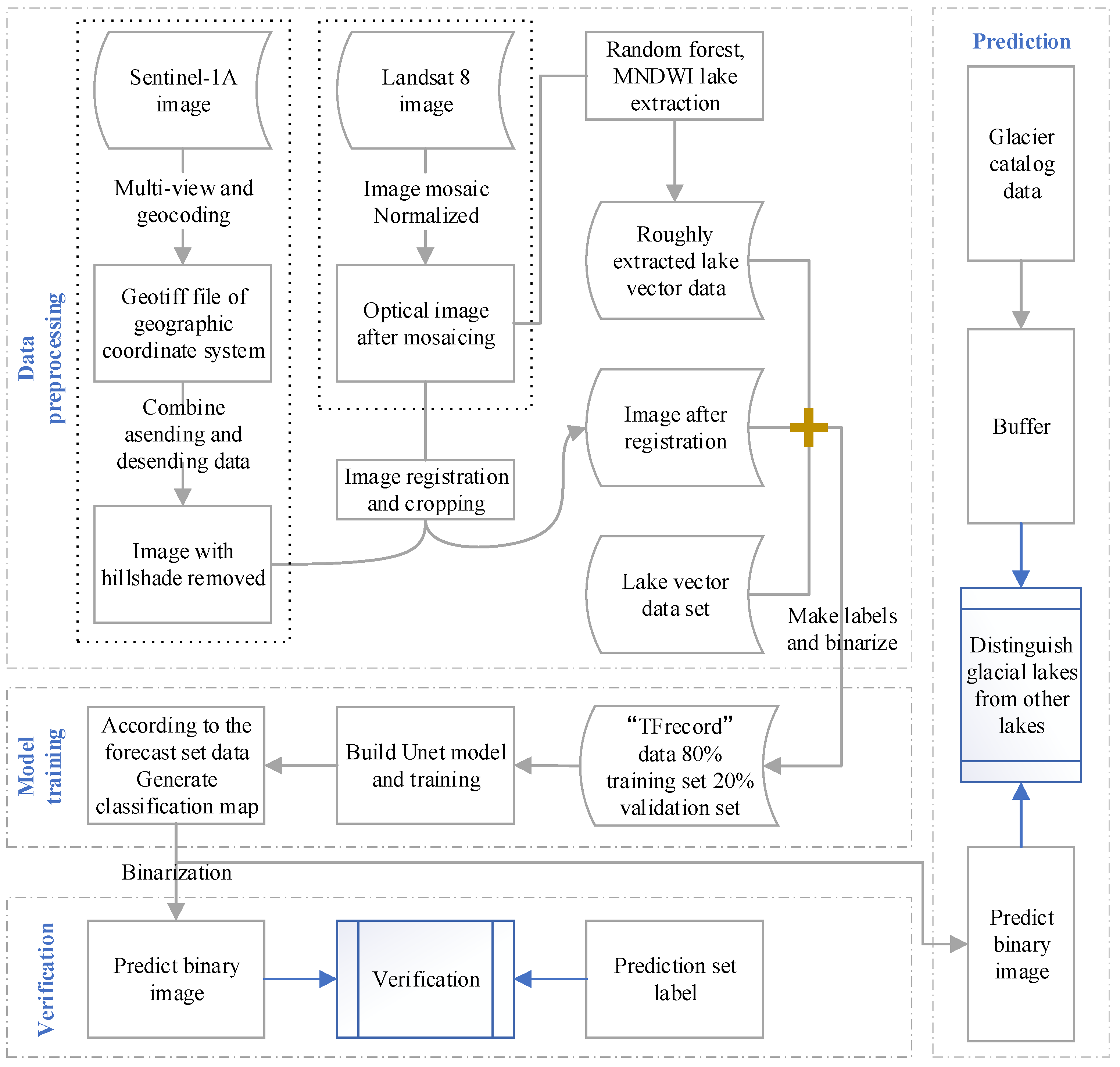
4.1. Experimental Technical Scheme

Figure 3 shows the automatic GL contour extraction procedure used in this study. The method used in this study is advantageous in the following areas. (1) This DL method is an automatic extraction scheme, and the trained model is relatively easy to use. (2) This method is capable of accurately and effectively extracting the contours of large and small lakes and highly capable of distinguishing rivers and lakes and requires only minimal postediting. (3) This method integrates the advantages of SAR and optical remote sensing images and performs well in extracting the contours of cloud-covered and frozen lakes.

The GL dataset used in the experiment was produced by eliminating data for lakes based on the glacial zones. Furthermore, other little GLs with a range less than a certain threshold were excluded also. While this dataset is suitable for most GL research, it is manifestly unreliable for training a DL model. DL training requires images to be segmented into blocks. The larger the image blocks are, the larger the required random-access memory and video memory as well as the computational load during DL training are. The image block size also dictates the size of the receptive field of the model and affects its ability to perceive correlated pixels. Because Landsat 8 image blocks have seven channels and Sentinel-1A image blocks have one channel, the image block size in this study was set to 512 × 512 × (7 + 1). While the pure background samples were eliminated in the establishment of the training set, the positive sample images in the training set still contained a large number of unlabelled lakes. If left untreated, these lakes would have been included in the negative sample areas during training, which would have significantly affected the accuracy and predictive capacity of the model. In addition, there was a certain interval between the time when the images used by the authors of the GL dataset were collected and the time when this study was conducted. During this time interval, the GLs underwent slight morphological changes, and the contours of some GLs were altered. As a result, the GL dataset could not be directly used. Thus, in this study, SAR images were introduced as an adjunct to Landsat 8 images. The contours of the lakes were approximately extracted using the MNDWI (at a threshold greater than 0.1) and the random forest (RF) algorithm. Moreover, the Landsat 8 bands 4, 5, and 6 were conjoined to enhance the lake information, and the lakes were then visually interpreted. This approach was implemented primarily to increase the number of samples and include the non-GLs in the samples as well as to correct the GL contour information inconsistent with the images.

4.2. Data Processing

Cloud cover significantly interferes with target extraction. SAR is capable of penetrating clouds and detecting lake ice and has been extensively used in lake-related research. In this study, IW-mode Sentinel-1A GRD amplitude images, collected mainly in September and October, were used. SAR is a side-looking imaging radar. As a result, SAR images have inherent problems such as close-range compression, shadows, layovers, and foreshortening. In particular, in mountainous areas, there are large areas of shadows whose reflected signals are similar to those of lakes, making it difficult for SAR to effectively distinguish them. Due to volume scattering and refraction, the reflected radar signals of GLs are extremely weak. GLs are in low-reflection areas in both ascending- and descending-orbit images. In view of this situation, ascending- and descending-orbit images were combined in this study to remove the shadows cast by mountains. Figure 4 shows a comparison of images before and after the removal of the shadows cast by mountains. Figure 4A,B shows an ascending-orbit image of a scene and a descending-orbit image of the same scene, respectively. Figure 4C shows the image obtained by removing the shadows cast by mountains based on a combination of the ascending- and descending-orbit images. It is difficult to determine the upper-bound radar reflectivity recorded in Sentinel-1A amplitude images. As a result, the radar reflectivity recorded in these images cannot be normalized. To avoid the exploding gradient problem during DL model training and considering that the radar reflectivity of GLs is low (digital number: <0.02), reflectivity values greater than 1 are all set to 1 in this study. Figure 4D shows the image obtained after reflectivity adjustments. In the transformed SAR amplitude image, the information on the body of water differs significantly from that on other surface features. (The images in Figure 4A–C are all greyscale equalized images).

The Sentinel-1A GRD data used in this study contained no geographic coordinates. Thus, geographic coordinates were generated with the 30-metre Shuttle Radar Topography Mission geocoder in the software GAMMA. According to the user manual of GAMMA, a geocoding accuracy within 0.1 pixel can meet the requirements of image mosaicking. However, there is a prevalent distortion error of 1–2 pixels between Sentinel-1A and Landsat 8 images, which significantly interferes with the extraction of GL contours. Thus, in this study, the mutual information method was employed to extract GL contours from the two types of remote sensing images of different sources registered based on homonymous points [31]. Mutual information, an important concept in systems theory, describes the correlations between two targets. The following shows the mutual information calculation equations for images:

$$p_i=h_i/({\displaystyle \sum _{i=1}^{N-1}{h}_i})$$

(14)

$$H(Y)=-{\displaystyle \sum _{i=0}^{N-1}{p}_i\log p_i}$$

(15)

$$H(X,Y)=-{\displaystyle \sum _{x,y}{p}_{XY}(x,y)\log p_{XY}(x,y)}=H(X)\cup H(Y)$$

(16)

$$MI(X,Y)=H(X)+H(Y)-H(X,Y)$$

(17)

where $h_i$ is the total number of occurrences of pixel $i$, $p_i$ is the probability of occurrence of pixel $i$, $H(Y)$ is the entropy value of image $Y$, $H(X,Y)$ is the combination entropy of images $(X,Y)$ and $MI(X,Y)$ is the mutual information value of images $(X,Y)$ (the higher $MI(X,Y)$ is, the more strongly the two images are correlated with each other). In this study, homonymous points were selected using images of seven Landsat 8 bands and SAR images. In addition, gross-error points are removed. The two types of remote sensing images of different sources are effectively registered based on cubic interpolation, and the pixel error is reduced to below one pixel.

4.3. Result

Deep learning methods with powerful fitting ability can meet the requirements of the extraction of lake (including GL) contours, and their accuracy is far higher than that of conventional methods (e.g., index thresholds and ML). These methods perform relatively well in distinguishing rivers and lakes and require only minimal manual correction to produce the contours of lakes and determine their areas at high accuracy. Deep learning methods used in the manuscript integrated SAR images with optical images. This significantly optimizes such phenomena as frozen lake surfaces and cloud cover, which in turn improves the sensitivity of the model, considerably reduces the numbers of false positives and false negatives in predictions, and significantly increases the IoU score for lake contour extraction. This method offers a new means for time-series monitoring of lakes.

In this study, the contours of lake waters were extracted while relatively satisfactorily avoiding river information. However, the extracted contours contained not only those of GLs but also those of a large number of other lakes. In a strict sense, GLs are defined as natural bodies of water supplied chiefly by modern glacial meltwater or formed by accumulation of water in depressions between moraine ridges [2]. This study focuses on the application of DL to GL contour extraction. Therefore, in this study, lakes within 10 km from glaciers were treated as GLs (manually eliminating incorrectly extracted broken river patterns), and the glacier data in the Second Glacier Inventory Dataset of China published by Liu and Xu in 2012 [30] were used. Figure 5 shows the distribution of the GLs in south-eastern Tibet extracted using the U-Net + All method. There are 8262 GLs in south-eastern Tibet, 86.8% of which are smaller than 0.1 km² in area. The distribution patterns of the perimeters and areas of the GLs are similar, suggesting that the GLs are generally circular or oval in shape and that relatively few GLs are narrow and long. The GLs in the study area were primarily concentrated at high altitudes. Most (89.5%) of the GLs were distributed at altitudes of 4500–5500 m.

5. Discussion

5.1. Result Analysis

The experimental data were divided into three sets, namely, a training set, a validation set, and a prediction set. Some images of south-eastern Tibet were used as training and validation data. The remaining data were used as a prediction set to analyze the GL contour extraction. Data for another three areas were selected as a prediction set to evaluate the experimental results (see

Table 1. Landsat-8 and Sentinel-1A remote sensing images used in this study (If the remote sensing satellite is Landsat-8, the Path/raw No. column represents the orbit number of the satellite. If the remote sensing satellite is Sentinel-1, it indicates the number of images used. The “Image explanation” column explains the image usage and cloud cover).

Remote Sensing Satellite	Date (YYYY-MM-DD)	Path/Row No.	Image Explanation
Landsat 8 Operational Land Imager (OLI)	2015-09-29 and 2015-10-31	133/38, 39, 40, and 41	Training set 0.4% < cloud cover < 17.0%
	2015-10-06 and 2015-11-23	134/38, 39, and 40	Training set 1.6% < cloud cover < 8.0%
	2015-10-13	135/38, 39, and 40	Training set 4.0% < cloud cover < 15.0%
	2015-10-20 and 2015-11-21	136/38, 39, 40, and 41	Validation and training sets 1.6% < cloud cover < 3.0%
	2015-10-11 and 2015-10-27	137/38, 39, 40, and 41	Prediction set 2.3% < cloud cover < 20.0%
	2015-10-02 and 2015-10-18	138/39 and 40	Prediction set 2.2% < cloud cover < 4.9%
	2015-10-02 and 2015-10-21	138/37, 141/39, and 143/39	Prediction set (used for evaluation) 0.13% < cloud cover < 4.4%
Sentinel-1A in ascending orbit	2015-09 and 2015-10	Images covering 23 scenes of the same area	SAR amplitude images Interferometric wide swath (IW) mode
Sentinel-1A in descending orbit	2015-09 and 2015-10	Images covering 20 scenes of the same area	SAR amplitude images IW mode

for details). This experimental scheme can effectively examine the transfer ability of the model and prevent the validation set from losing its function in examining the generalization ability of the model as the frequency of training increases.

To demonstrate the efficacy of DL in extracting mountainous GL contours, some images in the validation set were used to conduct a comparison experiment. Figure 6 shows the experimental results (L and S refer to Landsat 8 and Sentinel-1A images, respectively). The MNDWI, a common water index algorithm [14], ameliorated the problem associated with the NDWI—that water information contains excessive nonwater information. In the experiment, thresholds were calculated and selected using Otsu’s method [32]. Lake contours were extracted from each image using an optimum threshold. In addition, the RF algorithm, a strong learner for image classification commonly used in ML, was used. A total of 200 trees were established. There were as many positive samples as negative samples. Each type of sample covered 1.4 million points. Each point contained information on seven Landsat 8 bands. Sklearn [33] (Sourced from the France. Sklearn is a free software machine learning library for the Python programming language) was called upon for training. The labels and predicted classification results for the images in the validation set showed the following: (1) the DL method produced the best predictions with Landsat 8 and Sentinel-1A images as classification images. This method performed relatively well in identifying frozen and ice-free lakes and yielded almost no misidentifications; (2) with only Landsat 8 images as base images for training, the DL method performed similarly well in identifying GL contours but was relatively weak in identifying frozen lakes; (3) lake contours were relatively satisfactorily extracted with the MNDWI. However, the results contained a large number of shadows cast by mountains. Moreover, it was difficult to accurately describe the contours of frozen lakes using the MNDWI; (4) compared to the MNDWI, the RF algorithm performed better in identifying shadows cast by mountains and frozen lakes when used to extract lake contours. However, the RF algorithm yielded a large number of misidentifications in low-reflectivity areas and even identified the null-value areas in the images as lakes. Evidently, for production and application, the MNDWI and the ML method are suitable only for the approximate extraction of GL contours and perform relatively well in approximately classifying lake waters with no or a small number of samples and, thus, can significantly facilitate the establishment of labels. However, when used to produce vector data, these methods still require extensive manual postediting. Furthermore, these methods produce relatively large errors in identifying some frozen and cloud-covered bodies of water.

DL showed a high fitting ability in image classification. This method not only accounted for the reflection values of pixels in various bands but also was able to comprehensively take into consideration the relations between a pixel and its adjacent pixels as well as higher-dimensional multivariate information. Combining DL with GL contour extraction offers a new solution for GL contour extraction. In addition, as a result of the high fitting ability of DL as well as the use of SAR images as an adjunct to optical images in this experimental study, the extracted GL contours could be directly used in production with no or minimal editing. To further examine the importance of SAR images to GL contour extraction, the results produced by the DL model on the three datasets, namely, the training, validation, and prediction sets, are discussed in detail. The data in the training and validation sets were generated primarily by visual interpretation. The data in the prediction set as well as a small amount of data in the training and validation sets were generated by a combination of the MNDWI, the RF algorithm, and visual interpretation.

Figure 7 shows the values of four metrics, namely, the IoU score, accuracy, loss function, and Tversky index (an accuracy evaluation factor), for the DL model training process (U-Net + All indicates the use of U-Net to extract GL contours from combined optical and SAR images; U-Net + Optical indicates the use of U-Net to extract GL contours from only optical images; the curves in orange and green colour respect the changes in the validation and training sets, respectively). Due to the relatively large number of samples (1892 × 512 × 512 × 8 images) in the dataset, the U-Net model tended to converge after only 100 rounds of training. A comparison of multiple metrics found that the introduction of SAR images did not affect the convergence rate of the U-Net model. The addition of SAR images, to some extent, improved the overall performance of the U-Net model. The two methods were similar in terms of classification accuracy as a result of the relatively large number of background pixels in the predicted images. However, the U-Net + All method is superior to the U-Net + Optical method in terms of the IoU score and the Tversky index. This suggests that SAR images play a positive role in extracting GL contours.

The effects of SAR images on the ability of the model to extract GL contours were further investigated. Specifically, new data were used as a prediction set (see Table 1 for details) to ultimately evaluate the model. The results were comparatively analyzed to determine which images were better classified in the presence of SAR images. As demonstrated in

Table 2. Effects of SAR images on IoU.

#	Method	Number of Samples	Number of False Negatives	Number of False Positives	IoU > 0.5	Overall IoU
1	U-net + All	4960	92	397	3657	0.6397
2	U-net + Optical		242	768	3292	0.6014

, a total of 4960 samples were used in the comparison experiment. The IoU score was calculated by spatial association. For the U-Net + All (No. 1) method, SAR images were included as an adjunct to optical images. For the U-Net + Optical (No. 2) method, only optical images were used. The most notable difference between the two methods lay in the numbers of false positives and false negatives in the predictions. The prediction accuracy of the U-Net + All method was considerably higher than that of the U-Net + Optical method. In particular, the number of false positives generated by the U-Net + All method was only half that generated by the U-Net + Optical method. See Figure 8D for this case. Because the samples contained frozen lake and shadow areas with band information extremely similar to that on lake waters, the model was prone to identifying these areas as GL features in the absence of complementary SAR images, which affected its extraction accuracy. Similarly, the U-Net + All method performed better than the U-Net + Optical method in terms of the number of false negatives. See Figure 8A–C for details. In Figure 8A, the lakes were shadowed by clouds or mountains, and their features were similar to those of the shadows. In Figure 8B, the lakes were directly obstructed by clouds and, as a result, their visibility was inadequate. This type of optical remote sensing image is generally discarded. However, south-eastern Tibet is covered by clouds throughout the year. Only a relatively small number of usable images are available for this region each year. In principle, images with relatively low cloud cover are used. However, a small number of lakes in these images were still covered by clouds. In Figure 8C, the GL information was relatively complete. However, due to the differences in turbidity and the extent of freezing, there was a relatively significant difference between the spectral information of the GLs. Surface features with similar spectral information could be easily misidentified based on the features provided by the optical image alone. The aforementioned factors resulted in a sharp decline in the level of confidence in the identified lake waters. In this study, Sentinel-1A C-band images were used. The C-band has a wavelength of 5.6 cm and is naturally advantageous in penetrating clouds. Due to their low radar signal reflectivity, lakes appear as dark black spots in images. In this study, the maximum values of a combination of ascending- and descending-orbit images were used as common images, thereby eliminating most of the shadow areas and significantly improving the GL identification accuracy.

As an important metric for evaluating the image segmentation quality, the IoU plays an excellent descriptive role in evaluating the robustness and generalization ability of a model. Generally, an IoU score greater than 0.5 is used as a metric for correct segmentation. Table 2 summarizes the number of correctly predicted samples. The U-Net + All and U-Net + Optical methods correctly predicted 3657 and 3292 samples, respectively, accounting for 73.7% and 66.3% of all the samples, respectively. Overall, the IoU score on the prediction set was higher than that on the validation set. This is because when the labels are created for the prediction set, threshold segmentation and the RF algorithm are used as a complement to manual vectorization. The vectorized boundary pixels conform more to the segmentation results produced by U-Net. Figure 9 shows the distribution of the IoU scores. Because the lake areas greater than 1 km² in size exceeded the display range of the images, they were no longer shown in the images. Based on the scatter distribution, the extraction accuracies of the U-Net + All and U-Net + Optical methods increased with the lake area. The IoU score was generally greater than 0.8 for lakes greater than 0.1 km² in area, comparable to the manual vectorization accuracy. The U-Net + All method showed higher sensitivity than the U-Net + Optical method in extracting the contours of small lakes. The numbers of false positives and false negatives produced by the U-Net + All method were significantly smaller than those produced by the U-Net + Optical method. With regard to extraction of the contours of large lakes, the U-Net + All method performed better than the U-Net + Optical method in terms of the IoU score.

5.2. Defects in Current Work

Although the U-net + All method combines Landsat-8 and Sentinel-1 images to achieve large-scale and high-precision extraction of the glacier lake in the study area, there are still possible defects.

• In terms of data, Landsat-8 and Sentinel-1 do not match the space-time scale very well, especially as the 2015 Sentinel-1 images have different sizes, orbital information changes, and repeated observation is unstable. On the spatial scale, we have adopted the mutual information method to improve images matching relationship, but it is difficult to achieve complete uniformity on the time scale.
• The shadows cast by mountains in the Sentinel-1 images were removed in the experiment using a combination of ascending- and descending-orbit data, but there are still mountain shadow areas that cannot be removed, which have a negative impact on the experimental results.
• This experiment is the first attempt to reorganize the deep learning method to extract the glacial lakes in remote sensing images. The model used is relatively simple and can be further improved in subsequent experiments.

6. Conclusions

The mountainous areas of south-eastern Tibet are home to a profusion of GLs and are the focus of cryosphere and global climate change research. Because south-eastern Tibet experiences relatively abundant cloud cover throughout the year, it is difficult to rely solely on optical remote sensing means to obtain information on the dynamic changes in the GLs in this region. Combining SAR images in application can effectively improve the temporal resolution of collected data. To exploit the advantages of multispectral and SAR images to extract GL contours at high accuracy, an algorithm with a high generalization ability for extracting GL contours from combined optical and SAR images was established in this study by optimizing and improving the U-Net DL model.

The proposed DL automatic analysis method exhibited a relatively high generalization ability when applied to a large region of south-eastern Tibet and was far superior to conventional methods in terms of image segmentation accuracy related to GL contour extraction. In addition, the algorithm used in this study was notably advantageous in dealing with complex climatic conditions (frequent cloud cover). The technical method used in this study as well as the experimental results obtained can provide a reference and support for cryosphere and climate change research on south-eastern Tibet as well as GL disaster chain prevention and control.

References

1. Huggel, C.; Carey, M.; Emmer, A.; Frey, H.; Walker-Crawford, N.; Wallimann-Helmer, I. Anthropogenic climate change and glacier lake outburst flood risk: Local and global drivers and responsibilities for the case of lake Palcacocha, Peru. Nat. Hazards Earth Syst. Sci. 2020, 20, 2175–2193. [Google Scholar] [CrossRef]
2. Yao, X.; Liu, S.; Han, L.; Sun, M. Definition and classification systems of glacial lake for inventory and hazards study. J. Glaciol. Geocryol. 2017, 72, 1173–1183. [Google Scholar] [CrossRef] [Green Version]
3. Wen, J.; Han, P.F.; Zhou, Z.; Wang, X.S. Lake level dynamics exploration using deep learning, artificial neural network, and multiple linear regression techniques. Environ. Earth Sci. 2019, 78, 1–12. [Google Scholar] [CrossRef]
4. Cheng, Z.; Zhu, P.; Dang, C.; Liu, J. Hazards of Debris Flow due to Glacier-Lake Outburst in Southeastern Tibet. J. Glaciol. Geocryol. 2008, 030, 954–959. [Google Scholar]
5. Hewitt, K.; Liu, J. Ice-Dammed lakes and outburst floods, Karakoram Himalaya: Historical perspectives on emerging threats. Phys. Geogr. 2010, 31, 528–551. [Google Scholar] [CrossRef]
6. Westoby, M.J.; Glasser, N.F.; Brasington, J.; Hambrey, M.J.; Quincey, D.J.; Reynolds, J.M. Modelling outburst floods from moraine-dammed glacial lakes. Earth-Sci. Rev. 2014, 134, 137–159. [Google Scholar] [CrossRef] [Green Version]
7. Richardson, S.D.; Reynolds, J.M. An overview of glacial hazards in the Himalayas. Quat. Int. 2000, 65, 31–47. [Google Scholar] [CrossRef]
8. Roy, D.P.; Wulder, M.A.; Loveland, T.R.; Woodcock, C.E.; Allen, R.G.; Anderson, M.C.; Helder, D.; Irons, J.R.; Johnson, D.M.; Kennedy, R.; et al. Landsat-8: Science and product vision for terrestrial global change research. Remote Sens. Env. 2014, 145, 154–172. [Google Scholar] [CrossRef] [Green Version]
9. Yang, Y.; Liu, Y.; Zhou, M.; Zhang, S.; Zhan, W.; Sun, C.; Duan, Y. Landsat 8 OLI image based terrestrial water extraction from heterogeneous backgrounds using a reflectance homogenization approach. Remote Sens. Env. 2015, 171, 14–32. [Google Scholar] [CrossRef]
10. Bhardwaj, A.; Joshi, P.K.; Snehmani; Sam, L.; Singh, M.K.; Singh, S.; Kumar, R. Applicability of Landsat 8 data for characterizing glacier facies and supraglacial debris. Int. J. Appl. Earth Obs. Geoinf. 2015, 38, 51–64. [Google Scholar] [CrossRef]
11. Yang, C.; Wang, X.; Wei, J.; Liu, S. A dataset of glacial lake inventory of West China in 2015. China Sci. Data 2018, 3, 36–44. [Google Scholar]
12. Zhang, G.; Yao, T.; Xie, H.; Wang, W.; Yang, W. An inventory of glacial lakes in the Third Pole region and their changes in response to global warming. Glob. Planet. Chang. 2015, 131, 148–157. [Google Scholar] [CrossRef]
13. McFeeters, S.K. The use of the Normalized Difference Water Index (NDWI) in the delineation of open water features. Int. J. Remote Sens. 1996, 17, 1425–1432. [Google Scholar] [CrossRef]
14. Xu, H. Modification of normalised difference water index (NDWI) to enhance open water features in remotely sensed imagery. Int. J. Remote Sens. 2006, 27, 3025–3033. [Google Scholar] [CrossRef]
15. Bhardwaj, A.; Singh, M.K.; Joshi, P.K.; Snehmani; Singh, S.; Sam, L.; Gupta, R.D.; Kumar, R. A lake detection algorithm (LDA) using Landsat 8 data: A comparative approach in glacial environment. Int. J. Appl. Earth Obs. Geoinf. 2015, 38, 150–163. [Google Scholar] [CrossRef]
16. Wessels, R.L.; Kargel, J.S.; Kieffer, H.H. ASTER measurement of supraglacial lakes in the Mount Everest region of the Himalaya. Ann. Glaciol. 2002, 34, 399–408. [Google Scholar] [CrossRef] [Green Version]
17. Chen, F.; Zhang, M.; Tian, B.; Li, Z. Extraction of Glacial Lake Outlines in Tibet Plateau Using Landsat 8 Imagery and Google Earth Engine. IEEE J. Sel. Top. Appl. Earth Obs. Remote Sens. 2017, 10, 4002–4009. [Google Scholar] [CrossRef]
18. Barbieux, K.; Charitsi, A.; Merminod, B. Icy lakes extraction and water-ice classification using Landsat 8 OLI multispectral data. Int. J. Remote Sens. 2018, 39, 3646–3678. [Google Scholar] [CrossRef]
19. Luo, J.; Sheng, Y.; Shen, Z.; Li, J.; Gao, L. Automatic and high-precise extraction for water information from multispectral images with the step-by-step iterative transformation mechanism. J. Remote Sens. 2009, 013, 604–615. [Google Scholar]
20. Tom, M.; Aguilar, R.; Imhof, P.; Leinss, S.; Baltsavias, E.; Schindler, K. Lake ice detection from sentinel-1 sar with deep learning. Isprs Ann. Photogramm. Remote Sens. Spat. Inf. Sci. 2020, 5, 409–416. [Google Scholar] [CrossRef]
21. Zhang, Y.; Zhang, G.; Zhu, T. Seasonal cycles of lakes on the Tibetan Plateau detected by Sentinel-1 SAR data. Sci. Total Env. 2020, 703, 135563. [Google Scholar] [CrossRef] [PubMed]
22. Zhang, B.; Zhang, R.; Liu, G.; Liu, Q.; Cai, J.; Yu, B.; Fu, Y.; Li, Z. Monitoring of Interannual Variabilities and Outburst Regularities Analysis of Glacial Lakes at the End of Gongba Glacier Utilizing SAR Image. Geomat. Inf. Sci. Wuhan Univ. 2019, 44, 1054–1064. [Google Scholar]
23. Hanshaw, M.N.; Bookhagen, B. Glacial areas, lake areas, and snow lines from 1975 to 2012: Status of the cordillera vilcanota, including the Quelccaya Ice Cap, northern central Andes, Peru. Cryosphere 2014, 8, 359–376. [Google Scholar] [CrossRef] [Green Version]
24. Ronneberger, O.; Fischer, P.; Brox, T. U-net: Convolutional networks for biomedical image segmentation. Lect. Notes Comput. Sci. Incl. Subser. Lect. Notes Artif. Intell. Lect. Notes Bioinform. 2015, 9351, 234–241. [Google Scholar]
25. Zhou, Z.; Siddiquee, M.M.R.; Tajbakhsh, N.; Liang, J. Unet++: A nested u-net architecture for medical image segmentation. Lect. Notes Comput. Sci. Incl. Subser. Lect. Notes Artif. Intell. Lect. Notes Bioinform. 2018, 11045 LNCS, 3–11. [Google Scholar]
26. Chen, L.C.; Zhu, Y.; Papandreou, G.; Schroff, F.; Adam, H. Encoder-decoder with atrous separable convolution for semantic image segmentation. In Proceedings of the Lecture Notes in Computer Science (including Subseries Lecture Notes in Artificial Intelligence and Lecture Notes in Bioinformatics); Springer: Berlin/Heidelberg, Germany, 2018; Volume 11211 LNCS, pp. 833–851. [Google Scholar]
27. Xin, X.; Yao, T.; Ye, Q.; Guo, L.; Yang, W. Study of the Fluctuations of Glaciers and Lakes around the Ranwu Lake of Southeast Tibetan Plateau using Remote Sensing. J. Glaciol. Geocryol. 2009, 31, 19–26. [Google Scholar]
28. Liu, S.; Shang, D.; Ding, Y.; Han, H.; Zhang, Y.; Wang, J.; Xie, C.; Ding, L.; Li, G. Glacier Variations since the Early 20th Century in the Gangrigabu Range, Southeast Tibetan Plateau. J. Glaciol. Geocryol. 2005, 27, 55–63. [Google Scholar]
29. Liu, S.; Shangguan, D.; Ding, Y.; Han, H.; Xie, C.; Zhang, Y.; Li, J.; Wang, J.; Li, G. Glacier changes during the past century in the Gangrigabu m ountains, southeast Qinghai-Xizang (Tibetan) Plateau, China. Ann. Glaciol. 2006, 43, 187–193. [Google Scholar] [CrossRef] [Green Version]
30. Liu, S.; Xu, J. The second glacier inventory dataset of China (version 1.0) (2006–2011). Natl. Tibet. Plateau Data Cent. 2012. [Google Scholar] [CrossRef]
31. Chen, H.M.; Arora, M.K.; Varshney, P.K. Mutual information-based image registration for remote sensing data. Int. J. Remote Sens. 2003, 24, 3701–3706. [Google Scholar] [CrossRef]
32. Ostu, N. A threshold selection method from gray-histogram. IEEE Trans. Syst. Man. Cybern. 1978, 9, 62–66. [Google Scholar]
33. Pedregosa, F.; Varoquaux, G.; Gramfort, A.; Michel, V.; Thirion, B.; Grisel, O.; Blondel, M.; Prettenhofer, P.; Weiss, R.; Dubourg, V.; et al. Scikit-learn: Machine Learning in Python. J. Mach. Learn. Res. 2011, 12, 2825–2830. [Google Scholar]
Figure 1. U-Net model used to extract GL contours.
Remotesensing 12 04020 g001
Figure 2. Distribution of the lakes in the study area.
Remotesensing 12 04020 g002
Figure 3. Technical procedure for extracting GL contours.
Remotesensing 12 04020 g003
Figure 4. Removal of the shadows cast by mountains based on a combination of ascending- and descending-orbit Sentinel-1A images. (A) The ascending-orbit image. (B) The descending-orbit image. (C) Combination of the ascending- and descending-orbit images. (D) Normalized image.
Remotesensing 12 04020 g004
Figure 5. Extracted GLs contours and count the distribution pattern of GLs in south-eastern Tibet.
Remotesensing 12 04020 g005
Figure 6. Comparison of multiple methods in terms of extraction of mountainous GL contours.
Remotesensing 12 04020 g006
Figure 7. Effects of the introduction of SAR images on the training and validation sets.
Remotesensing 12 04020 g007
Figure 8. Effects of SAR images on GL contour extraction. (AD) These images respectively show the extraction effect of L+S+Unet and L+Unet methods in different scenarios.
Remotesensing 12 04020 g008
Figure 9. Distribution of the IoU scores.
Remotesensing 12 04020 g009