Article

Analyzing Daily Estimation of Forest Gross Primary Production Based on Harmonized Landsat-8 and Sentinel-2 Product Using SCOPE Process-Based Model

1
Global Change Research Institute of the Czech Academy of Sciences, 60300 Brno, Czech Republic
2
Institute of Bio- and Geosciences: Agrosphere (IBG-3), Forschungszentrum Jülich GmbH, 52425 Jülich, Germany
*
Author to whom correspondence should be addressed.
Current address: Bělidla 986/4a, 60300 Brno, Czech Republic.
Remote Sens. 2020, 12(22), 3773; https://doi.org/10.3390/rs12223773
Submission received: 8 September 2020 / Revised: 10 November 2020 / Accepted: 12 November 2020 / Published: 17 November 2020

Abstract

:
Vegetation top-of-canopy reflectance contains valuable information for estimating vegetation biochemical and structural properties, and canopy photosynthesis (gross primary production (GPP)). Satellite images allow studying temporal variations in vegetation properties and photosynthesis. The National Aeronautics and Space Administration (NASA) has produced a harmonized Landsat-8 and Sentinel-2 (HLS) data set to improve temporal coverage. In this study, we aimed to explore the potential and investigate the information content of the HLS data set using the Soil Canopy Observation of Photosynthesis and Energy fluxes (SCOPE) model to retrieve the temporal variations in vegetation properties, followed by the GPP simulations during the 2016 growing season of an evergreen Norway spruce dominated forest stand. We optimized the optical radiative transfer routine of the SCOPE model to retrieve vegetation properties such as leaf area index and leaf chlorophyll, water, and dry matter contents. The results indicated percentage differences less than 30% between the retrieved and measured vegetation properties. Additionally, we compared the retrievals from HLS data with those from hyperspectral airborne data for the same site, showing that HLS data preserve a considerable amount of information about the vegetation properties. Time series of vegetation properties, retrieved from HLS data, served as the SCOPE inputs for the time series of GPP simulations. The SCOPE model reproduced the temporal cycle of local flux tower measurements of GPP, as indicated by the high Nash–Sutcliffe efficiency value (>0.5). However, GPP simulations did not significantly change when we ran the SCOPE model with constant vegetation properties during the growing season. This might be attributed to the low variability in the vegetation properties of the evergreen forest stand within a vegetation season. We further observed that the temporal variation in maximum carboxylation capacity had a pronounced effect on GPP simulations. We focused on an evergreen forest stand. Further studies should investigate the potential of HLS data across different forest types, such as deciduous stand.

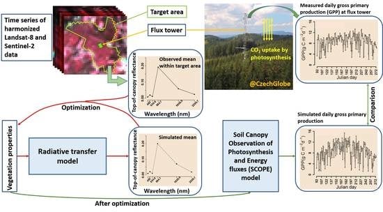
Graphical Abstract

1. Introduction

Vegetation is an essential component of the terrestrial ecosystems that interacts with the atmosphere through the carbon and water cycles. The leaf stomata regulate the release of water by transpiration and the uptake of atmospheric carbon dioxide by photosynthesis. The sum of the gross photosynthesis by all leaves measured at the ecosystem scale is known as gross primary production (GPP) [1]. GPP, together with respiration, governs the exchange of CO 2 between the biosphere and atmosphere, thereby providing the capacity of the terrestrial ecosystems to offset anthropogenic CO 2 emissions [2]. Reliable estimation of spatio-temporal GPP variation in various terrestrial ecosystems is crucial because the changes of GPP over time reflect vital processes in plants and provide information about the plant–atmosphere feedback resolved over a large area [3,4].
Spatio-temporal variations in GPP can be quantified using either data-driven or data-assimilation approaches [5]. Data-driven approaches establish an empirical model between ground measurements of GPP (e.g., GPP partitioned from flux tower measurements of net ecosystem exchange [6]) and other explanatory variables that are commonly derived from remote sensing data (satellite images). The empirical model extrapolates the spatio-temporal variations in GPP. Among the widely-used explanatory variables, vegetation indices (VIs) (e.g., normalized difference vegetation index (NDVI), enhanced vegetation index (EVI), and photochemical reflectance index (PRI)) are the indices that have been mostly often used in various studies [7,8,9,10,11]. However, there are several limitations when using VIs as an explanatory variable connected with the upscaling of flux tower measurements [12]. For instance, the leaf greenness approximated from VIs (e.g., by means of NDVI and EVI) may not be necessarily proportional to the photosynthetic capacity and rate. Environmental stressors may affect the photosynthesis rate even during the early stages without the appearance of any significant visual symptoms at the leaf (e.g., leaf color change) or canopy levels (e.g., leaf area index change). This creates challenges to relating the maximum photosynthesis capacity to maximum vegetation greenness. The majority of VIs are derived at the leaf level (e.g., PRI as a proxy for the leaf conversion efficiency of absorbed light); therefore, further upscaling from the leaf to the canopy level is not always feasible due to the additional confounding effects of the canopy structure on VIs.
Data-assimilation approaches calibrate a process-based model (PBM) against the data on the output variables, e.g., flux tower measurements. The calibrated PBM is then used to estimate the spatio-temporal variations in GPP [13,14,15,16]. The limitations of VIs in the data-driven approach do not occur when adopting the data-assimilation approaches for GPP estimation. PBM can predict GPP by simulating various plant physiological responses to climatic and atmospheric conditions and stand structural properties [16,17,18,19], which are not explicitly included in the data-driven approach.
Overall, a PBM is required to effectively interpret remote sensing data and exploit their full potential for estimating GPP variations in various terrestrial ecosystems. Among the developed PBMs, the Soil Canopy Observation of Photochemistry and Energy fluxes (SCOPE, [19]) model has been widely used in various applications, all attempting to contribute to a better understanding and interpretation of remote sensing data over vegetation, for instance, by: (1) simulating multiple satellite radiances through coupling with an atmosphere radiative transfer model [20,21]; (2) retrieving biochemical and structural vegetation properties [22,23,24]; and (3) estimating vegetation functioning variations and their biases [20,25,26]. Further extensions of the SCOPE model have been recently proposed and examined in various ecosystems to improve their performance [27,28,29]. However, attempts to use the SCOPE model to estimate temporal variation in GPP of a forest stand by exploring the potential of combined remote sensing data are lacking.
The SCOPE model integrates radiative transfer, micrometeorology, and plant physiology to perform land surface process (e.g., GPP) simulations [20]. The SCOPE model uses a modular architecture, making it flexible and allowing the use of different modules as standalone instances. The radiative transfer module (RTMo) can be calibrated, i.e., a data-assimilation approach, against the surface reflectance obtained from remote sensing data to optimize its input parameters. These optimized parameters are the retrieved vegetation biochemical and structural properties. The retrieved information, together with the time series of meteorological variables, can be then directly used as inputs for the SCOPE model for GPP estimation. In general, the vegetation properties at one point in time can yield a rough estimate of GPP. However, temporal variations in the vegetation properties (i.e., vegetation phenology) are also needed to reflect the vegetation responses to climate variability and were found to improve the temporal GPP estimated by the SCOPE model [20,22].
Accurate description of the temporal variations in vegetation properties depends on the availability of rich time series of high quality remote sensing data. A single sensor may not provide the needed temporal coverage due to cloud cover and sensor temporal revisit limitations. More than 300 Earth observation satellites for optical imaging are orbiting the Earth, allowing us to combine observations from multiple sensors for improved temporal coverage. However, a simple combination of observations does not result in smooth spectral time series, e.g., due to the differences in radiometric characteristics and mismatch in spatial resolution between the sensors. It is not always suitable to assess the vegetation phenology and retrieve consistent time series of vegetation characteristics from the combined datasets. Recently, the National Aeronautics and Space Administration (NASA) produced the harmonized Landsat and Sentinel (HLS) data set by combining the surface reflectance data from the Operational Land Imager (OLI) and Multi-Spectral Instrument (MSI) sensors aboard Landsat-8 and Sentinel-2 satellites, respectively [30], to further improve the temporal resolution of the combined product. In HLS data, a smooth spectral time series is produced by accounting for the differences in spatial resolution, sensor-to-sensor differences in atmospheric correction approaches, and view geometry and radiometric characteristics of spectral bands. The potential of HLS time series data has not yet been fully explored with respect to GPP estimations. Recently, Lin et al. [31] applied a data-driven approach using HLS data to evaluate GPP variations in natural vegetation types. However, the full potential of HLS time series data has not yet been explored with respect to GPP estimation using data-assimilation approaches. The objective of this study was to fill this gap by assimilating multi-sensor spectral information obtained from the HLS data within the SCOPE model to retrieve the temporal variations in biochemical and structural vegetation properties to evaluate the improvement in GPP estimation. This research addresses the following two questions: (1) What information is preserved or lost in the retrieval of vegetation properties using multispectral HLS data? (2) What improvement in the GPP estimation can be expected by providing the SCOPE model with the temporal variations in the vegetation properties? We assumed that HLS multispectral data can provide sufficient information for retrieval of vegetation properties. However, whether such information can improve GPP estimation needs more investigation. We aimed to gain insights regarding these two aspects.

2. Study Area

We used measurements recorded at the Bílý Kříž ecosystem station in the Czech Republic, which is part of the Czech Carbon Observation System (CzeCOS; http://www.czecos.cz/) network. The Bílý Kříž site is situated in the northeast Czech Republic ( 49 30 07 . 474 N, 18 32 12 . 777 E) at an altitude of 875 m above sea level on a 13 southwest-oriented planar slope that is approximately 100 m downslope of a mountain crest extending from west to east [32]. This site is a Class 2 candidate site of the Integrated Carbon Observation System (ICOS) (www.icos-cp.eu) and it regularly contributes to the FLUXNET dataset labeled as CZ-BK1 [33]. The site is predominated by a Norway spruce (Picea abies (L.) H. Karst) forest stand that represents the evergreen needle leaf forest vegetation class. The stand had a mean height of 17 m and the age of 35 years at the end of the 2016 vegetation growing season. This site is located in a moderately cold, humid, and precipitation-rich temperate climatic zone [34]. The soil at the Bílý Kříž site is an Entic Podsol type with a texture ranging from sandy loam to sandy clay with a 15–35% clay fraction [35]. The site is equipped with an eddy covariance flux tower system that has been measuring the energy and trace gas fluxes between the ecosystem and the atmosphere since 2004. We investigated the retrieval of vegetation properties and the estimation of GPP from remote sensing data for the 2016 vegetation growing season (April to September) when airborne hyperspectral data and ground measurements of vegetation biochemical and structural properties were available for this site.

3. Materials and Methods

3.1. Data

3.1.1. Remote Sensing Data

We obtained a time series of 39 images at 30 m resolution from the HLS data product that covered the study area from 1 April to 30 September 2016. The HLS data are atmospherically corrected with spatial coregistration, bidirectional reflectance distribution function normalization, and spectral bandpass adjustments of Landsat-8 MSI and Sentinel-2 OLI sensors. The MSI surface reflectance bands are also adjusted to Landsat-8 characteristics by applying the spectral response function of the OLI sensor. The HLS surface reflectance data product is distributed globally within the Sentinel-2 tiling system and is abbreviated as S30 (obtained from Sentinel-2 MSI sensor) and L30 (obtained from Landsat-8 OLI sensor). For more information about the processing of MSI and OLI observations within the HLS data product, the reader is referred to Skakun et al. [36] and Claverie et al. [30]. We included the time series of HLS data available between 11:38 to 11:54 a.m. Central European Time during the 2016 vegetation growing season. Further filtering of the HLS data was performed based on the quality indicators using NDVI and near infrared (NIR) reflectance (see Section 3.2 for more details).
We also obtained the hyperspectral airborne data over the study area. We compared the retrieval of vegetation properties from both airborne and HLS data to examine if multispectral HLS bands preserve the required information compared to hyperspectral bands. The airborne data were acquired around local solar noon between 11 a.m. and 2 p.m. on 31 August 2016 with two push broom spectroradiometers (Compact Airborne Spectrographic Imager (CASI) and shortwave Infrared (SWIR) Airborne Spectrographic Imager (SASI) from Itres Ltd., Calgary, AB, Canada) onboard the Flying Laboratory of Imaging Systems operated by the Global Change Research Institute [37,38]. The CASI operates in the visible and NIR regions between 372 and 1044 nm (72 spectral bands with a sampling distance of 9.4 nm) and a nominal spatial resolution of 1.0 m. SASI operates in the shortwave infrared region between 957 and 2442 nm (100 spectral bands with a sampling distance of 15 nm) and nominal spatial resolution of 2.5 m. The airborne data were corrected radiometrically (using the factory calibration coefficients in RCX software (Itres Ltd., Calgary, AB, Canada)), geometrically (using GeoCorr software (Itres Ltd., Calgary, AB, Canada)), and atmospherically (using ATCOR-4 software [39]), and combined into a single hypercube according to the processing chain established at Global Change Research Institute [37]. The quality of the atmospheric corrections was evaluated by comparing the airborne spectra extracted for homogeneous artificial surfaces with spectral signatures measured in the field during the overflight, which produced maximum differences of 3% in NIR and SWIR wavelengths for some targets (Figure S1). Both HLS and airborne data were used to retrieve vegetation properties at the Bílý Kříž site (Section 3.2). For this purpose, we extracted the surface reflectance of the vegetation canopy, i.e., top-of-canopy (TOC) reflectance, from the target area delineated by the ecosystem boundary (Section 3.1.2).

3.1.2. Ground Measurements

We obtained half-hourly eddy covariance (EC) measurements of net ecosystem exchange (NEE) to predict half-hourly GPP and standardized meteorological variables for the spruce forest stand during the 2016 growing season. The EC technique [40] was applied to measure turbulent fluxes of CO 2 at the Bílý Kříž forest site. The EC system consisted of Gill ultrasonic anemometer (HS-50, Gill Instruments, Hampshire, UK) and a LI-COR infrared gas analyzer (LI-7200, LI-COR, Lincoln, NE, USA), and was installed on a meteorological tower at 20.5 m as of 1 October 2013 and moved to 25 m as of 7 June 2016 above ground level. The EC raw data measured at 20 Hz were processed using spike detection and removal [41], time lag compensation, sonic temperature correction [42], and high- [43,44] and low [45]-frequency spectral corrections. Coordinates were rotated using the planar-fit method [46]. Fluxes were computed at half-hourly time intervals using the block averaging method. Fetch filtering was applied to exclude half hours for which more than 30% of the signal originated from outside of the target area. This was achieved by comparing fetch distance at a given upwind direction with estimated distance providing 70% contribution to the EC fluxes using footprint modeling [47,48]. Fetch distance for all directions is represented as an ecosystem boundary, i.e., the target area (Figure 1), that delimits the area that is sufficiently homogeneous considering the canopy height and the species represented (Norway spruce at the Bílý Kříž site).
All EC processing and calculations were performed using EddyPro software (v6.2.0, LI-COR, Lincoln, NE, USA). A thorough data quality checking procedure was applied to EC measurements in this study using R package openeddy (R Core Team, 2020; https://github.com/lsigut/openeddy; see McGloin et al. [32] for details). Measured CO 2 fluxes were filtered based on the friction velocity threshold computed using the moving point method [49]. After this filtering, half-hourly CO 2 fluxes were assumed to represent the NEE (µmol CO2 m−2 s−1). Gaps were filled using marginal distribution sampling [50] and NEE was partitioned into GPP (hereafter, GPP EC ) and ecosystem respiration according to Lasslop et al. [6] using the R package REddyProc [51]. Half-hourly GPP EC were then aggregated to daily sums of carbon, expressed as g C m−2 s−1.
Meteorological variables included half-hourly data of air temperature (T a , in C ), TOC incoming shortwave radiation (Rin, in W m−2), TOC incoming longwave radiation (Rli in W m−2), vapor pressure deficit (e a , in hPa), air pressure (p, in hPa), and wind speed (u, in m−2) for each day in the vegetation growing season of 2016. We additionally obtained half-hourly soil water content (SWC, in %) from the nine sensors installed at a 5 cm depth at different locations within the target area. For each half-hour, SWC values from all nine sensors were averaged to obtain the representative value of soil moisture of the target area. The half-hourly meteorological variables, mean SWC, along with HLS-, CASI-, and SASI-derived information served as the inputs to the SCOPE model to estimate (or simulate) half-hourly GPP, which was aggregated to daily sums of carbon (Section 3.3). We refer to simulated GPP as GPP SIM hereafter. We validated daily GPP SIM against daily GPP EC . We also compared daily GPP SIM with daily means of half-hourly measurements of meteorological variables to show the relationship between them. Table 1 lists the summary statistics of daily meteorological variables during the 2016 vegetation growing season.
Additionally, we obtained ground measurements of vegetation properties characterizing spruce forest conditions at the site, which were collected during a joint ground/airborne campaign on 31 August 2016. The location of the field sampling plots was pre-determined by previously existing forest inventory plots established by the Institute of Forest Ecosystem Research (IFER), Czech Republic, in the vicinity of the ecosystem station. The coordinates of the central point of each plot were measured using a differential global positioning system. The measured biochemical vegetation properties included leaf chlorophyll content ( C ab ), leaf carotenoids content ( C ca ), leaf water content ( C w ), and leaf dry matter content ( C dm ). The biochemical properties were measured in a laboratory (leaf pigments were extracted according to Porra et al. [52]) for needles sampled from the top and bottom part of the crown of three representative trees selected at each sample plot. The measured structural property was the leaf area index L A I , which was determined at the plot level using a Plant Canopy Analyser LAI-2200 instrument (LI-COR, Lincoln, NE, USA). More details about the ground measurements and data pre-processing are reported in Homolová et al. [38]. These ground measurements were compatible with airborne hyperspectral data acquired on 31 August 2016. For this study, we used the minimum, mean, and maximum measurements of three plots that were located inside and right at the edge of the target area (Figure 1). These three plots represented a Norway-spruce-dominated forest stand. Table 2 provides the means of the measured vegetation properties. We validated the retrieved vegetation properties against the measured means.

3.2. Retrieval of Vegetation Properties Time Series Using HLS and Airborne Data and the SCOPE Model

The SCOPE model is an integration of four modules [19] that interact with each other to simulate the optical properties and physiological state of plants. The modules include: (a) the radiative transfer module in the optical domain (RTMo) for simulating TOC reflectance by tracking the propagation of incident solar and sky radiation; (b) the radiative transfer module for thermal radiation (RTMt), to simulate TOC outgoing thermal radiation; (c) energy balance and biochemical routines to simulate heat fluxes and photosynthesis; and (d) a radiative transfer module that simulates the TOC spectrum for chlorophyll fluorescence (RTMf). In this study, we inverted the RTMo module as a separate model to retrieve vegetation properties and finally simulated the photosynthesis (i.e., GPP SIM ) using forward SCOPE modeling.
The leaf level model PROSPECT5 [53] and the canopy-level reflectance model 4SAIL (scattering by arbitrary inclined leaves) [54] are combined in the RTMo model of SCOPE. The PROSPECT5 model simulates the leaf-level reflectance and transmittance from the input biochemical leaf properties. Leaf-level optical properties are further upscaled on canopy scale by accounting for the canopy architecture using the 4SAIL model. We also incorporated the effect of soil background (soil brightness and SWC) on the simulated reflectance using the brightness-shape-moisture (BSM) submodel as previously suggested [20,21]. Table 2 provides the input parameters of the RTMo model and the BSM submodel.
We evaluated the quality of HLS data before the retrieval of vegetation properties. For the 2016 vegetation growing season, we downloaded HLS data for 39 days. The HLS data are distributed with a per-pixel quality layer to mask the pixels of poor quality (e.g., due to the presence of clouds or other processing artifacts). However, the accuracy of the internal cloud mask is insufficient [30], and its use may lead to the omission of cloud detection. This was also the case for our study area for some days. Therefore, we did not use the internal cloud mask of the HLS data, but propose our method for filtering the time series based on the empirical threshold of NDVI and NIR reflectance. We only considered pixels to be of high quality when the NDVI varied between 0.5 and 0.99 (vegetation pixels) and the NIR reflectance between 0.1 and 0.4 (typical spruce canopy reflectance values as, for instance, reported by Rautiainen et al. [55]). Thresholds were set based on our previous experience with the reflectance characteristics of Norway spruce in the study area during the growing season. For each day, we calculated the mean of TOC reflectance in each HLS band within the target area if more than 50% of the pixels were of high quality (fulfilling both the NDVI and NIR thresholds). Of the original 39 days, 14 days were retained after the filtering. For the retrieval, we selected six HLS bands relevant for studying the vegetation properties that were common in both Sentinel-2 and Landsat-8 data. These selected bands were blue (482 nm), green (561.4 nm), red (654.6 nm), NIR narrow (864.7 nm), and two shortwave infrared bands (SWIR 1 (1608.9 nm) and SWIR 2 (2200.7 nm)). Table 3 shows the 14 days with the percentage of high quality pixels within the target area.
For each of the 14 days with HLS data, we used an optimization method to invert the RTMo model against mean TOC reflectance to retrieve the dynamics of the vegetation properties, as described in van der Tol et al. [24]. To tune the parameters, we used nonlinear least squares optimization, implemented in the MATLAB (the MathWorks Inc., Natick, MA, USA) built-in function “lsqnonlin”, to minimize a cost function that calculated the sum of squared differences between the simulated and measured mean TOC reflectance in the selected six HLS optical bands. In this study, we chose to retrieve five biochemical parameters ( C ab , C w , C dm , C s , and C ca ; Table 2) and three structural parameters ( L A I , leaf inclination distribution function ( L I D F ) and leaf structural parameter (N); Table 2). To run the optimization method, prior information, i.e., range, mean, and standard deviation of each vegetation property to be retrieved (Table 2) was needed. We used non-informative prior information following Verhoef et al. [21] and Bayat et al. [22] to ensure the significant impact of the measured HLS reflectance on the retrieved parameters. We used the middle of the total range (i.e., (lower bound + upper bound)/2) as a prior mean of each vegetation property. Assuming uniform prior distribution over the range between the lower and upper bound produced values of standard deviation equal to 1 / 12 0.3 times the range of each vegetation property. We fixed the SWC based on the measurements of mean SWC within the target area measured at the observation time of HLS data (Section 3.1.2 and Table 3). We used the BSM submodel to describe soil background reflectance. The BSM submodel is based on the library of global soil vectors [56], which is extended via a brightness-shape component and SWC effect. This has two main advantages: (1) the model can simulate soil reflectance, providing an effective alternative to soil spectrum measurements; and (2) the model can scale the dry soil spectrum for any given SWC. Further, the BSM submodel can be inverted to retrieve BSM input parameters (soil brightness (B), L a t , and L o n ) from the given dry soil spectrum. We took advantage of this possibility and retrieved these three input parameters by inverting the BSM submodel against a dry soil reflectance extracted from the airborne data.
We also calculated a mean TOC reflectance within the target area from the airborne hyperspectral data acquired on 31 August 2016. It was used to retrieve the vegetation properties using the RTMo inversion, where we used the same non-informative prior information of the vegetation properties and the BSM input parameters as we used for HLS data. We further used the ground measurements (Table 2) to compare the retrieved vegetation properties obtained from HLS and airborne data.

3.3. Simulating Gross Primary Production Using SCOPE Model

After retrieving the time series of the forest’s biochemical and structural properties, we set up the SCOPE model to simulate the half-hourly GPP SIM during the 2016 vegetation growing season. These half-hourly values were summed to daily GPP SIM values calculated in g C m−2 s−1. The SCOPE model inputs for GPP SIM included: (1) half-hourly meteorological variables, i.e., R in , R li , T a , p, e a , and u (introduced in Section 3.1.2); (2) vegetation properties, i.e., C ab , C w , C dm , C s , C ca , L A I , L I D F , and N (Table 2); (3) maximum rate of carboxylation ( V cmax , in μmol m−2 s−1 ); and (4) the Bell–Berry stomatal parameter m. We ran the SCOPE model with three scenarios to investigate the impact of information retrieved from the HLS data on the accuracy of GPP SIM :
“Fixed” scenario: We assumed no variations in the retrieved vegetation properties during the growing season. We fixed them either at the available measured means (Table 2) or at the prior means. L I D F a and L I D F b were fixed at –0.35 and –0.15, respectively, showing the spherical characteristics of Norway spruce [54]. We further fixed V cmax = 80 μmol m−2 s−1 and m = 9, which are the typical values for evergreen needle leaf species as suggested in the SCOPE model. This scenario allowed us to monitor the temporal variation in GPP SIM determined by changes in radiation and atmospheric demand.
“HLS info” scenario: We used the time series of vegetation properties retrieved from the HLS data as the inputs to the SCOPE model. In this scenario, we also fixed V cmax and m at the typical values for evergreen needle leaf species, since these two cannot be directly retrieved from the optical reflectance [20].
“HLS info & var Vcmax” scenario: We used the same time series of retrieved vegetation properties as in the HLS info scenario. Here, instead of using a fixed typical value of V cmax , we estimated its time series from the retrieved time series of C ab from the HLS data. For this, we used the empirical relationship between V cmax [μmol m−2 s−1] and C ab [μg cm−2] proposed by Houborg et al. [57] for C 3 plants:
V cmax = a × C ab + b ,
where a = 2.529 and b = –27.34. This scenario allowed us to monitor the temporal variation in GPP SIM when we relied on optical domain information both directly from the retrieved vegetation properties and indirectly from the empirical relationships.

3.4. Statistical Evaluation of Model Performance

We determined the performance of the SCOPE simulations using statistical criteria that evaluated the efficiency with which the SCOPE reproduced the flux tower GPP EC . These criteria provided a measure of the SCOPE model efficiency in simulating daily GPP SIM over the 2016 vegetation growing season. We used the following criteria:
Root mean square error ( RMSE ) = 1 n i = 1 n ( z i y i ) 2 ,
Nash - Sutcliffe efficiency ( NSE ) = 1 i = 1 n ( z i y i ) 2 i = 1 n ( z i z ¯ ) 2 ,
Correlation coefficient ( COR ) = i = 1 n ( z i z ¯ ) ( y i y ¯ ) i = 1 n ( z i z ¯ ) 2 i = 1 n ( y i y ¯ ) 2 ,
where n is the number of daily simulated GPP SIM ( y i ) and daily measured GPP EC ( z i ), and z ¯ and y ¯ represent the mean over the vegetation growing period. The RMSE criterion has the unit of GPP. A low RMSE indicates high accuracy. It is appropriate to compare the simulations under different scenarios (Section 3.3). The NSE [58] can range from to 1. An NSE value close to 1 indicates a perfect match of simulations to the observations. Following Dumont et al. [59], we assumed that an NSE ≥0.5 indicates adequate accuracy in GPP SIM . The COR represents the linear relationship between simulations and observations, and can vary from –1 to 1. We also used Equations (3) and (4) to evaluate the efficiency with which the RTMo produced TOC reflectance on each day. In this case, z i and y i represent the observed and the RTMo-simulated HLS/airborne TOC reflectance at the wavelength i, respectively.
We compared the vegetation properties retrieved from the HLS data with those retrieved from the airborne data, and the measurements using the percentage difference:
Percentage difference = A i B i A i B i 2 × 100 ,
where A i and B i represent the ith vegetation property retrieved from HLS data and airborne data, respectively. For comparison with the measurements, B i represents the ith measured vegetation property.

4. Results

4.1. Variation in Observed Top-Of-Canopy Reflectance

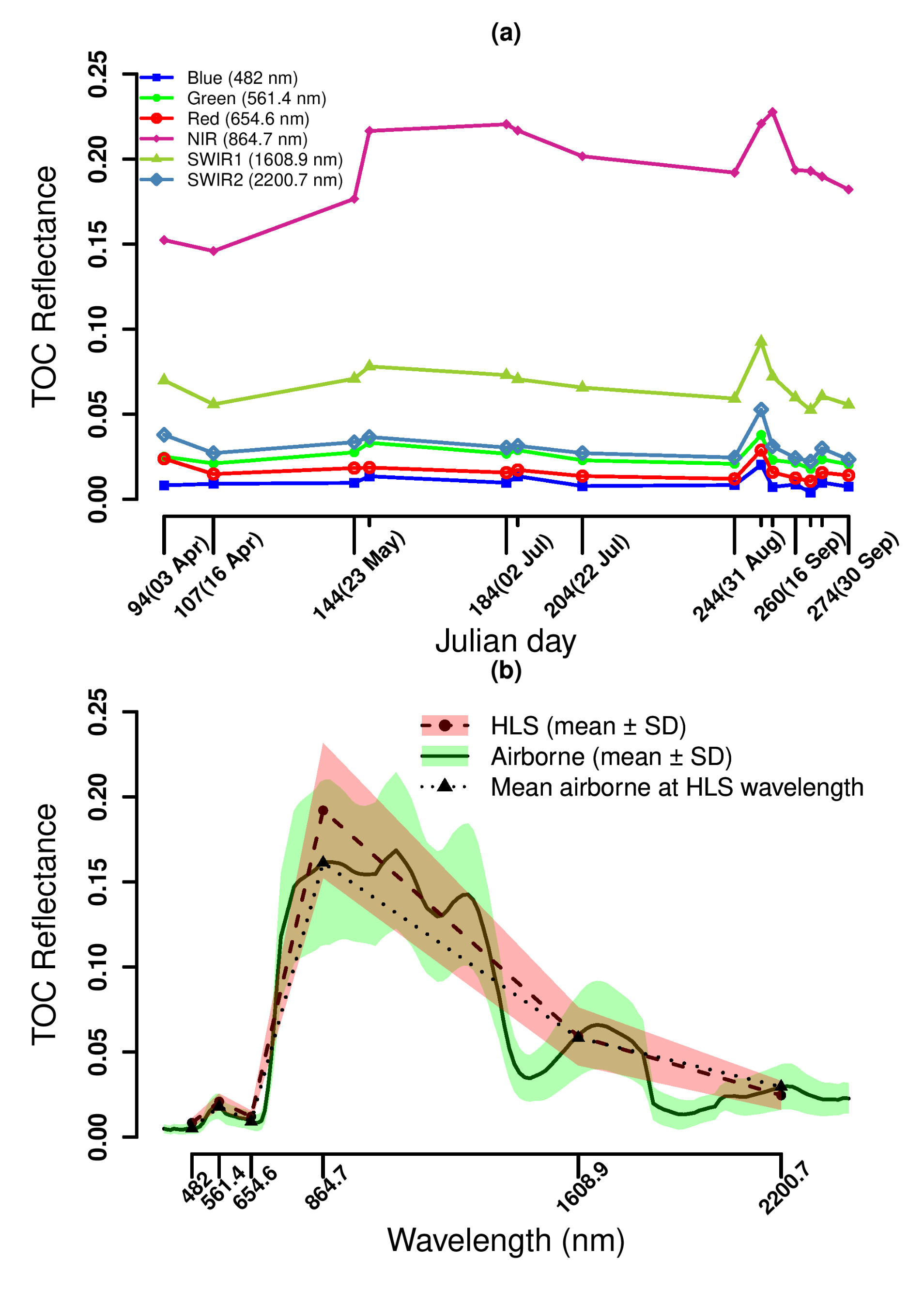
Figure 2a shows the temporal variation in the mean TOC reflectance extracted from the HLS data within the target area. The highest variation was observed in the NIR band with increasing NIR reflectance from the start of the vegetation growing seasons, which then stabilized mid-season, and decreased at the end of vegetation growing season. Other bands exhibited the same pattern, but with smaller variations in the magnitude of reflectance compared to the NIR band.
The observed temporal variation in the TOC reflectance likely did not occur due to the variation in L A I because the evergreen Norway spruce species can be expected to have stable L A I (Section 4.3) throughout the year. Instead, change in leaf age distribution caused temporal variation in the reflectance. Both young and mature leaves contribute to the TOC reflectance when captured from the top of the crown by the sensors of HLS data. Young leaves, in particular, start becoming greener from the beginning of the vegetation growing season, and then they stay sufficiently green until September and then start browning. This phenological development of the young leaves was likely the cause of variation in the TOC reflectance observed in this study.
Figure 2b compares the mean and standard deviation, showing the variability of TOC reflectance within the target area, extracted from the HLS and airborne data acquired on 31 August 2016. To facilitate comparison, we also plotted the airborne reflectance resampled at the band centers of the HLS data. Both the HLS and airborne data exhibited similar magnitudes of mean TOC reflectance, with slightly higher NIR reflectance (0.19) in the HLS compared to airborne data (0.16). We found that both the HLS and airborne data exhibited similar variability within the target area even though the stand variability was poorly captured in the HLS data with coarse spatial resolution compared to the airborne data.

4.2. Simulation of TOC Reflectance

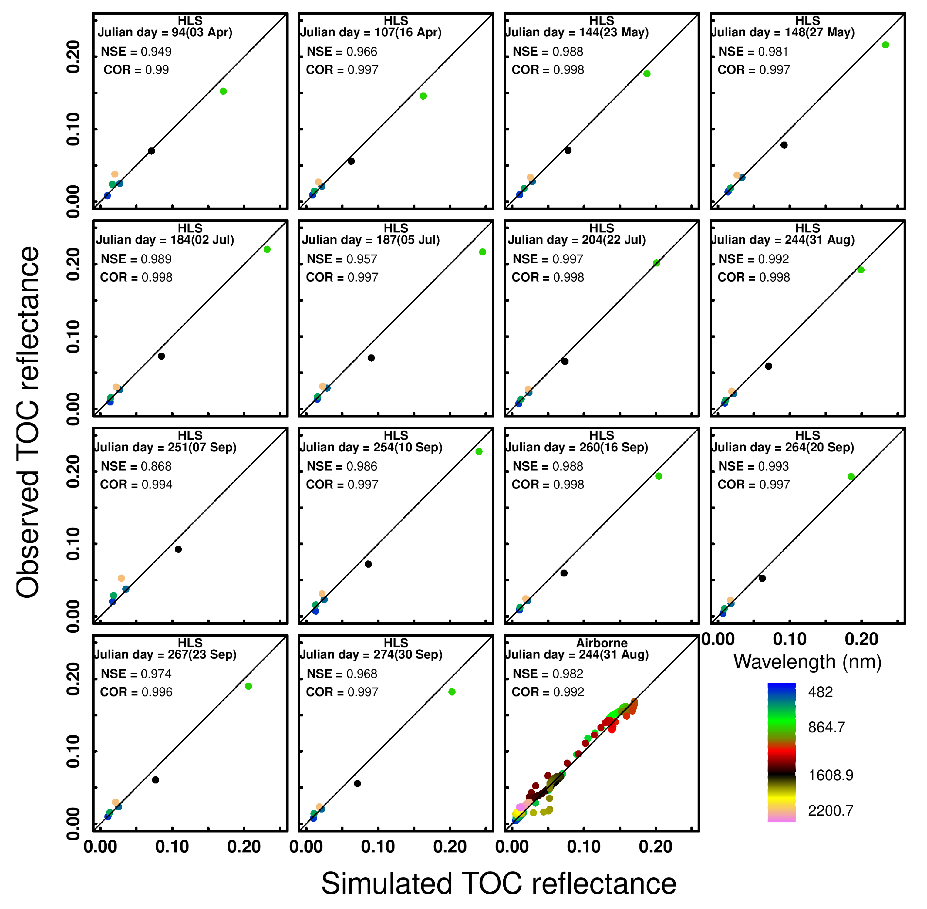
We assessed the performance of the RTMo model in retrieving vegetation properties by: (1) using the goodness-of-fit measured between the simulated and observed TOC reflectance; and (2) comparing the retrieved with the measured vegetation properties (Section 4.3). Figure 3 illustrates the goodness of fit using COR and NSE, and provides a spectral comparison between the observed mean TOC reflectance (by HLS and airborne) and the simulated TOC reflectance (by the RTMo model) for all 14 days during the vegetation growing season. We found that the NSE was close to one on each day, indicating a perfect match between the simulated and observed TOC reflectance. Strong positive correlations between simulations and observations were indicated by a COR value close to one. These showed that the RTMo model was able to successfully reproduce the observed HLS and airborne TOC reflectance. We presented the observed and simulated TOC reflectance curves for the selected Julian days in Figure S2.

4.3. Retrieval of Vegetation Properties

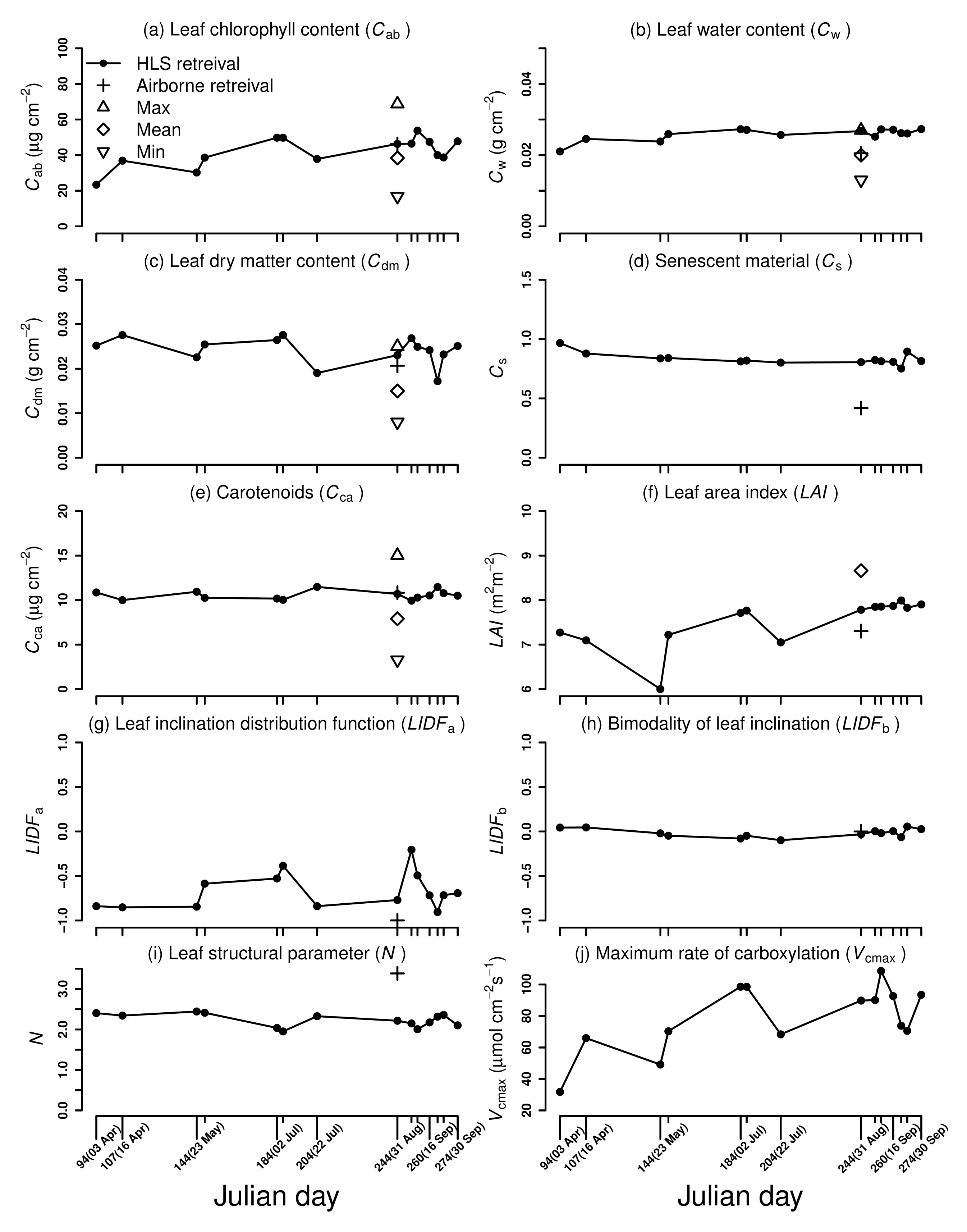
Figure 4 illustrates the variations in the retrieved vegetation properties during the 2016 vegetation growing season. For comparison, Figure 4 also includes the retrieval from airborne data on 31 August 2016, and the minimum, maximum, and mean values obtained from the ground measurements. The y-axis represents the non-informative prior distribution range of each vegetation property (Table 2). An optimization process constrained the RTMo input by the TOC reflectance (either HLS or airborne). Each vegetation property was retrieved in a narrow range during the growing season, indicating the reduction in prior uncertainty after the optimization.
From HLS data, we were able to retrieve the vegetation properties at least once per month. Only in June was it not possible to find a reliable observation for use in the retrieval. These retrievals provide insight into the temporal patterns of vegetation properties. Except for C ab and C dm , we did not observe any apparent temporal variation in any of the studied vegetation properties. We retrieved a low estimate of C ab at the start of the growing season (23.4 μg cm−2 on 3 April), which increased to 50 μg cm−2 in mid-season (5 July), and then showed an overall decreasing trend toward the end. C dm followed a similar pattern as C ab during the growing season, i.e., both decreased or increased together between any two successive days. The retrieval of L A I showed consistency during the growing season, and we retrieved the L A I between 7 and 8 m2 m−2, except for 23 May, where it dropped to 6 m2 m−2. This drop is, however, not an unrealistic estimate of L A I for Norway spruce.
We obtained the percentage difference between the vegetation properties retrieved from the HLS and airborne data using Equation (5) to show the similarity between them. We observed low percentage differences in most of the vegetation properties. The percent differences for C ab , C dm , C ca , and L A I were less than 10%, with the lowest being 0.3% for C ab . C w and L I D F a showed a difference of 25%. The maximum differences in C s and N were observed at 63% and 42%, respectively.
Based on the percentage difference, we compared the vegetation properties retrieved from the HLS data on 31 August with the mean of the available ground measurements (Table 2 and Figure 4). We found that the percentage differences for C ab , C w , C dm , C ca , and L A I were less than 30%. We found the lowest difference for L A I , with 7%, whereas C ab showed a difference of 17%. These percentage differences appear to be acceptable given the aggregated effect of the target area compared with the three separate plots of measurements (Figure 1). Moreover, all the retrieved vegetation properties were within the minimum and maximum, i.e., the range of the measurements (Figure 4), indicating the retrievals were reasonable, at least on 31 August 2016.

4.4. Simulations of GPPSIM with SCOPE Model

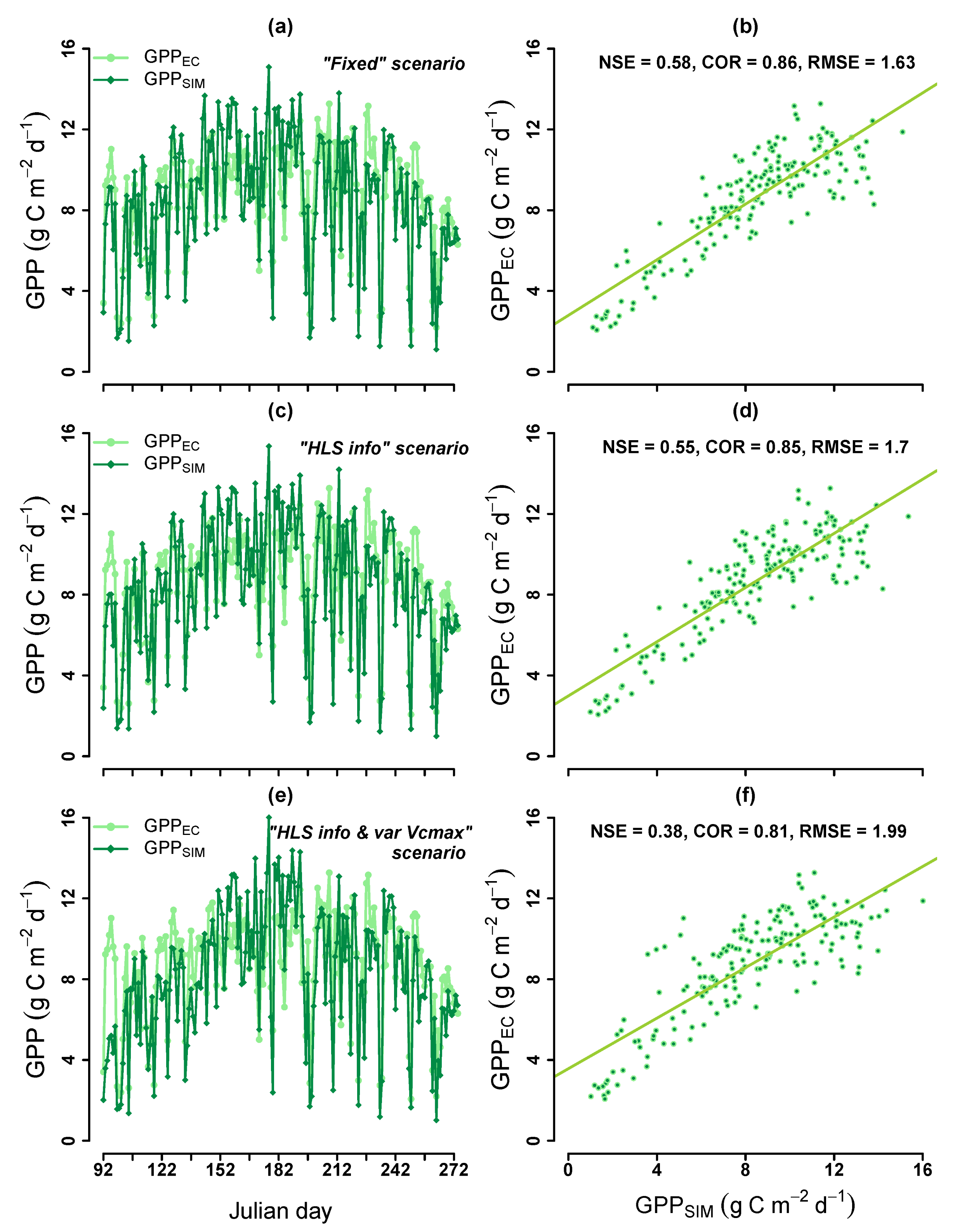
Finally, we evaluated the performance of the SCOPE model by comparing the simulated daily GPP SIM with the daily GPP EC measured during the 2016 vegetation growing season. Figure 5 illustrates the temporal variation in daily GPP SIM for three designed scenarios (Section 3.3), together with the daily GPP EC .
We also present the scatterplots between daily GPP SIM and GPP EC to show their correlation between them. Under both the Fixed and HLS info scenarios, daily GPP SIM closely followed the daily GPP EC (Figure 5a,c), visually indicating the accuracy of GPP SIM . The quantitative description of the GPP SIM accuracy was confirmed with the estimated NSE value (Equation (3)), which was found to be greater than 0.5 for both scenarios. The high NSE value indicated the sufficient quality of the predictive power of the SCOPE model for simulating gross primary production. We, however, observed some under- and over-estimation in GPP SIM compared to the GPP EC . The scatterplots (Figure 5b,d) further explain the positive linear relationship between GPP SIM and GPP EC , with the value of COR being high (close to 0.9 for both scenarios). This high value indicated that the variation of GPP SIM between consecutive days were synchronized with that of GPP EC . We also concluded that both Fixed and HLS info scenarios led to similar magnitude and variation in daily GPP SIM during the vegetation growing season, and both scenarios quantitatively produced similar NSE values, together with similar RMSE values (Equation (2)).
Under the HLS info & var Vcmax scenario, we estimated V cmax from the time series of C ab (Equation (1)) as ranging from 31.8 to 108.5 μmol m−2 s−1 during the vegetation growing season (Figure 4j). The variation in V cmax resulted in the synchronization between daily GPP SIM and GPP EC , but substantial differences in their magnitudes (Figure 5e) compared to the other two scenarios. These indicated the decrease in the quality of the predictive power of the SCOPE model for GPP SIM . The drop in NSE below 0.5 and the increase in RMSE provided quantitative evidence of this decrease. The linearity in the relationship between GPP SIM and GPP EC also reduced, which resulted in a drop in COR (Figure 5f).
Most of the variability in daily GPP SIM can be explained by its response to meteorological variables. We showed that R in was the main driver of GPP SIM , with strong dependence especially up to daily mean R in = 200 W m−2 (Figure 6a). The GPP SIM response to R in was further modified by T a (Figure 6b). The GPP SIM response to T a can be roughly separated to two regimes by a threshold of ≈13 C . The colder regime (<13 C ) was associated with generally lower GPP SIM than during the warmer regime (>13 C ). Most of the colder regime days occurred during the beginning of the growing season, whereas the warmer regime occurred during the core of the growing season. The GPP SIM values for the end of the growing season fell during both regimes but typically represented the lower end of the GPP SIM range within a given regime (Figure 6b). Although T a was the lowest mostly in the beginning of the growing season and could be expected to form the lower bound of the light response curve, GPP SIM values for the end of the growing season showed even lower values when accounting for R in .

5. Discussion

This study provided insight into the potential of using newly produced HLS data for the retrieval of temporal variations in vegetation properties using the RTMo model, and we investigated if these temporal variations could improve GPP SIM . In addition, we investigated the information contained about vegetation properties in the multispectral HLS data compared to hyperspectral airborne data.
The amount of HLS data contributing to the time-series was reduced by cloud coverage condition over the site. The cloud mask is not properly defined in the HLS data, and this was also observed in this study. The non-cloud pixels were defined based on the NDVI range (0.4 to 0.5) and NIR range (0.1 to 0.4). The NDVI range adopted in this study was based on the broad range of NDVI for vegetation, and the NIR range was based on our previous experience on the characteristics of Norway spruce during the growing period in the study area. The variations in these ranges can be observed for other species and the study period [60]. For example, the NIR reflectance can drop to below 0.1 outside the vegetation growing period and can rise to above 0.4 for grey alder tree species. Therefore, NDVI- and NIR-based filtering of cloud-free HLS data may be suitable at the local level and for shorter periods, like in this study. However, this filtering solution might be unsuitable if the study involves several tree species in a broad area and a longer study period. Therefore, the existing cloud mask of the HLS data, i.e., irrespective of tree species/land cover types, should be made more robust.
The RTMo model successfully reproduced the observed HLS and airborne TOC reflectance (Figure 3). The RTMo model is essentially a well-established combination of leaf-canopy radiative transfer models (PROSPECT5 leaf model and 4SAIL canopy reflectance model), which has been successfully used in numerous studies for the retrieval of vegetation properties. Therefore, the good fit between the observed and simulated TOC reflectance found in this study has already been reported in the literature [19,20,21,22,23,24,61,62,63,64,65,66,67].
We retrieved the time series of vegetation properties from the HLS data. We had a limited number of ground measurements for validation of the retrievals. However, the following points should be noted:
  • A temporal increase in C dm is positively correlated with C ab . A previous study, however, did not focus on the temporal aspects of evergreen as well as deciduous tree species, but also found a positive correlation between C dm and C ab [68].
  • We observed a good fit between the retrieved vegetation properties and the ground measurements (Section 4.3) on 31 August. At least for one day in the time series, we could therefore validate the retrievals from the HLS TOC reflectance. The retrieved C ab , however, did not exhibit substantial temporal variation. Nevertheless, these variations followed the characteristics of the evergreen tree species, which shows young leaf development phenology during the growing season. These findings agree with those of a previous study on the global spatio-temporal distribution of leaf chlorophyll [69], which highlighted the consistency in the temporal leaf chlorophyll profile of evergreen tree species across the year with an increasing concentration within new needles in spring.
Considering the points described above, we inferred a successful retrieval of vegetation properties from the HLS data. In a future study, these two points could be considered together for validation of retrievals, at least for evergreen tree species, if limited measurements are available.
We compared the retrievals from HLS and airborne data. The low percentage differences in most of the vegetation properties indicated that switching from hyperspectral to multispectral observations did not prominently influence the retrieval of vegetation properties in our case. In other words, the multispectral HLS data preserve a considerable amount of information about vegetation properties. This finding is in agreement with Croft et al. [70] who reported similarity between the C ab values over the range of tree species belonging to different biome types, retrieved from hyperspectral measurements and Landsat observations. Further, our finding is in line with Darvishzadeh et al. [71], who exploited the potential of Sentinel-2 data for the mapping of C ab of Norway spruce. Our study highlighted the potential of the newly produced HLS data set to monitor the vegetation properties by taking advantage of its denser time series.
We further examined if the time series of vegetation properties, retrieved from the HLS data, could improve the simulation of GPP SIM by the SCOPE model. We observed that both constant (Fixed scenario) and time-varying vegetation properties (HLS info scenario) led to almost identical GPP SIM during the vegetation growing season (Section 4.4). These results confirmed that the GPP SIM in Norway spruce is mainly driven by meteorological conditions (Figure 6). Therefore, the time-varying vegetation properties’ information could be significant for GPP SIM only when the tree is either under stress condition (e.g., due to drought) or exhibits strong temporal phenology (such as deciduous tree species). In a previous study, Bayat et al. [20] reported an improvement in temporal GPP SIM of the plant under stress using the time-varying vegetation properties input to the SCOPE model. In our study, the SCOPE model was mainly driven by the meteorological conditions because the Norway spruce did not show pronounced temporal variations in vegetation properties (Section 4.3) and were under no significant stress condition during the selected episode [32]. Therefore, constant vegetation properties were sufficient for simulating temporal GPP SIM with reasonable accuracy. We further observed the influence of time-varying V cmax (HLS info & var Vcmax scenario) on GPP SIM . We expected that some fluctuations in GPP SIM (Figure 5a,c) would be further improved with time-varying V cmax instead of using a constant value throughout the vegetation growing season. The time-varying V cmax , however, reduced the accuracy of GPP SIM (Figure 5f), which could be attributed to the empirical relationship of V cmax and C ab defined for C 3 plants (Equation (1)). A more robust empirical relationship between the C ab and V cmax must thus be defined for this site. A biome specific definition [72] could improve the estimation of V cmax , but this should be tested at the local site in a future study.

6. Conclusions

The present analysis showed the potential of the newly produced multispectral harmonized Landsat-8 and Sentinel-2 (HLS) data to retrieve time series of vegetation properties (i.e., biochemical and structural), which were further used as inputs to the Soil Canopy Observation, Photochemistry and Energy fluxes (SCOPE) model to simulate the time series of gross primary production GPP SIM . The study led to the following conclusions:
  • HLS data can provide the dense time series of surface reflectance at the desired locations because it combines data from two existing satellites: Landsat-8 and Sentinel-2. The results demonstrated that the HLS data are capable of preserving the needed information about vegetation properties. We investigated the retrieval only for one evergreen tree species. Nevertheless, our analysis has an important implication for the future use of HLS data for the dense time series retrieval of vegetation properties, which is needed for other tree species, such as deciduous species, showing strong temporal phenology.
  • We did not observe any improvement in GPP SIM using the time-varying vegetation properties retrieved from the HLS data. We observed the influence of the time-varying maximum rate of carboxylation ( V cmax ) on GPP SIM . However, the empirical relationship used to estimate V cmax from leaf chlorophyll content ( C ab ) decreased the accuracy of GPP SIM . Future studies need to redefine this empirical relationship.

Supplementary Materials

The following are available at https://www.mdpi.com/2072-4292/12/22/3773/s1.

Author Contributions

Conceptualization, R.R., B.B., P.L., and L.H.; methodology, R.R.; software, R.R., B.B., and P.L.; investigation, R.R., B.B., and P.L.; data curation, R.R., L.H., and L.Š.; Writing—Original draft preparation, R.R.; Writing—Review and editing, R.R., B.B., P.L., L.H., and L.Š. All authors have read and agreed to the published version of the manuscript.

Funding

This work was supported by: (1) the Global Change Research Institute of the Czech Academy of Sciences and the Ministry of Education, Youth and Sports of CR within the CzeCOS program, grant number LM2018123; (2) the Czech Science Foundation project “Radiation balance of forest stands of the Czech Republic”, grant number GJ17-05608Y. The co-author L.Š. was supported by the Ministry of Education, Youth and Sports of CR within Mobility CzechGlobe2 (CZ.02.2.69/0.0/0.0/18_053/0016924).

Conflicts of Interest

The authors declare no conflict of interest.

References

  1. Anav, A.; Friedlingstein, P.; Beer, C.; Ciais, P.; Harper, A.; Jones, C.; Murray-Tortarolo, G.; Papale, D.; Parazoo, N.C.; Peylin, P.; et al. Spatiotemporal Patterns of Terrestrial Gross Primary Production: A Review. Rev. Geophys. 2015, 3, 785–818. [Google Scholar] [CrossRef] [Green Version]
  2. Beer, C.; Reichstein, M.; Tomelleri, E.; Ciais, P.; Jung, M.; Carvalhais, N.; Rödenbeck, C.; Arain, M.A.; Baldocchi, D.; Bonan, G.B.; et al. Terrestrial Gross Carbon Dioxide Uptake: Global Distribution and Covariation with Climate. Science 2010, 329, 834–838. [Google Scholar] [CrossRef] [PubMed] [Green Version]
  3. Jung, M.; Verstraete, M.; Gobron, N.; Reichstein, M.; Papale, D.; Bondeau, A.; Robustelli, M.; Pinty, B. Diagnostic assessment of European gross primary production. Glob. Chang. Biol. 2008, 14, 2349–2364. [Google Scholar] [CrossRef]
  4. He, H.; Liu, M.; Xiao, X.; Ren, X.; Zhang, L.; Sun, X.; Yang, Y.; Li, Y.; Zhao, L.; Shi, P.; et al. Large-scale estimation and uncertainty analysis of gross primary production in Tibetan alpine grasslands. J. Geophys. Res. Biogeosci. 2014, 119, 466–486. [Google Scholar] [CrossRef] [Green Version]
  5. Xiao, J.; Chen, J.; Davis, K.J.; Reichstein, M. Advances in upscaling of eddy covariance measurements of carbon and water fluxes. J. Geophys. Res. Biogeosci. 2012, 117, G00J01. [Google Scholar] [CrossRef] [Green Version]
  6. Lasslop, G.; Reichstein, M.; Papale, D.; Richardson, A.D.; Arneth, A.; Barr, A.; Stoy, P.; Wohlfahrt, G. Separation of net ecosystem exchange into assimilation and respiration using a light response curve approach: Critical issues and global evaluation. Glob. Chang. Biol. 2010, 16, 187–208. [Google Scholar] [CrossRef] [Green Version]
  7. Patel, N.R.; Dadhwal, V.K.; Saha, S.K. Measurement and Scaling of Carbon Dioxide (CO2) Exchanges in Wheat Using Flux-Tower and Remote Sensing. J. Indian Soc. Remote. Sens. 2011, 39, 383–391. [Google Scholar] [CrossRef]
  8. Jung, M.; Reichstein, M.; Margolis, H.A.; Cescatti, A.; Richardson, A.D.; Arain, M.A.; Arneth, A.; Bernhofer, C.; Bonal, D.; Chen, J.; et al. Global patterns of land-atmosphere fluxes of carbon dioxide, latent heat, and sensible heat derived from eddy covariance, satellite, and meteorological observations. J. Geophys. Res. Biogeosci. 2011, 116, G00J07. [Google Scholar] [CrossRef] [Green Version]
  9. Yu, Q.; Wang, S.; Mickler, R.; Huang, K.; Zhou, L.; Yan, H.; Chen, D.; Han, S. Narrowband Bio-Indicator Monitoring of Temperate Forest Carbon Fluxes in Northeastern China. Remote Sens. 2014, 6, 8986–9013. [Google Scholar] [CrossRef] [Green Version]
  10. Verma, M.; Friedl, M.A.; Law, B.E.; Bonal, D.; Kiely, G.; Black, T.A.; Wohlfahrt, G.; Moors, E.J.; Montagnani, L.; Marcolla, B.; et al. Improving the performance of remote sensing models for capturing intra- and inter-annual variations in daily GPP: An analysis using global FLUXNET tower data. Agric. For. Meteorol. 2015, 214–215, 416–429. [Google Scholar] [CrossRef] [Green Version]
  11. Chen, B.; Ge, Q.; Fu, D.; Yu, G.; Sun, X.; Wang, S.; Wang, H. A data-model fusion approach for upscaling gross ecosystem productivity to the landscape scale based on remote sensing and flux footprint modelling. Biogeosciences 2010, 7, 2943–2958. [Google Scholar] [CrossRef] [Green Version]
  12. Lees, K.J.; Quaife, T.; Artz, R.R.E.; Khomik, M.; Clark, J.M. Potential for using remote sensing to estimate carbon fluxes across northern peatlands—A review. Sci. Total Environ. 2018, 615, 857–874. [Google Scholar] [CrossRef]
  13. Desai, A.R. Climatic and phenological controls on coherent regional interannual variability of carbon dioxide flux in a heterogeneous landscape. J. Geophys. Res. 2010, 115, G00J02. [Google Scholar] [CrossRef] [Green Version]
  14. Xiao, J.; Davis, K.J.; Urban, N.M.; Keller, K.; Saliendra, N.Z. Upscaling carbon fluxes from towers to the regional scale: Influence of parameter variability and land cover representation on regional flux estimates. J. Geophys. Res. Biogeosci. 2011, 116, G00J06. [Google Scholar] [CrossRef] [Green Version]
  15. Ran, Y.; Li, X.; Sun, R.; Kljun, N.; Zhang, L.; Wang, X.; Zhu, G. Spatial representativeness and uncertainty of eddy covariance carbon flux measurements for upscaling net ecosystem productivity to the grid scale. Agric. For. Meteorol. 2016, 230–231, 114–127. [Google Scholar] [CrossRef] [Green Version]
  16. Raj, R.; van der Tol, C.; Hamm, N.A.S.; Stein, A. Bayesian integration of flux tower data into a process-based simulator for quantifying uncertainty in simulated output. Geosci. Model Dev. 2018, 11, 83–101. [Google Scholar] [CrossRef] [Green Version]
  17. Constable, J.V.H.; Friend, A.L. Suitability of process based tree growth models for addressing tree response to climate change. Environ. Pollut. 2000, 110, 47–59. [Google Scholar] [CrossRef]
  18. Running, S.W. Testing Forest-BGC ecosystem process simulations across a climatic gradient in Oregon. Ecol. Appl. 1994, 4, 238–247. [Google Scholar] [CrossRef]
  19. Van der Tol, C.; Verhoef, W.; Timmermans, J.; Verhoef, A.; Su, Z. An integrated model of soil-canopy spectral radiances, photosynthesis, fluorescence, temperature and energy balance. Biogeosciences 2009, 6, 3109–3129. [Google Scholar] [CrossRef] [Green Version]
  20. Bayat, B.; van der Tol, C.; Verhoef, W. Integrating satellite optical and thermal infrared observations for improving daily ecosystem functioning estimations during a drought episode. Remote Sens. Environ. 2018, 209, 375–394. [Google Scholar] [CrossRef]
  21. Verhoef, W.; van der Tol, C.; Middleton, E.M. Hyperspectral radiative transfer modeling to explore the combined retrieval of biophysical parameters and canopy fluorescence from FLEX—Sentinel-3 tandem mission multi-sensor data. Remote Sens. Environ. 2018, 204, 942–963. [Google Scholar] [CrossRef]
  22. Bayat, B.; van der Tol, C.; Verhoef, W. Retrieval of land surface properties from an annual time series of Landsat TOA radiances during a drought episode using coupled radiative transfer models. Remote Sens. Environ. 2020, 238, 110917. [Google Scholar] [CrossRef]
  23. Bayat, B.; van der Tol, C.; Verhoef, W. Remote sensing of grass response to drought stress using spectroscopic techniques and canopy reflectance model inversion. Remote Sens. 2016, 8, 557. [Google Scholar] [CrossRef] [Green Version]
  24. van der Tol, C.; Rossini, M.; Cogliati, S.; Verhoef, W.; Colombo, R.; Rascher, U.; Mohammed, G. A model and measurement comparison of diurnal cycles of sun-induced chlorophyll fluorescence of crops. Remote Sens. Environ. 2016, 186, 663–677. [Google Scholar] [CrossRef]
  25. Timmermans, J.; Su, Z.; van der Tol, C.; Verhoef, A.; Verhoef, W. Quantifying the uncertainty in estimates of surface–atmosphere fluxes through joint evaluation of the SEBS and SCOPE models. Hydrol. Earth Syst. Sci. 2013, 17, 1561–1573. [Google Scholar] [CrossRef] [Green Version]
  26. Verrelst, J.; van der Tol, C.; Magnani, F.; Sabater, N.; Rivera, J.P.; Mohammed, G.; Moreno, J. Evaluating the predictive power of sun-induced chlorophyll fluorescence to estimate net photosynthesis of vegetation canopies: A SCOPE modeling study. Remote Sens. Environ. 2016, 176, 139–151. [Google Scholar] [CrossRef]
  27. Bayat, B.; van der Tol, C.; Yang, P.; Verhoef, W. Extending the SCOPE model to combine optical reflectance and soil moisture observations for remote sensing of ecosystem functioning under water stress conditions. Remote Sens. Environ. 2019, 221, 286–301. [Google Scholar] [CrossRef]
  28. Vilfan, N.; van der Tol, C.; Yang, P.; Wyber, R.; Malenovský, Z.; Robinson, S.A.; Verhoef, W. Extending Fluspect to simulate xanthophyll driven leaf reflectance dynamics. Remote Sens. Environ. 2018, 211, 345–356. [Google Scholar] [CrossRef]
  29. Yang, P.; Verhoef, W.; van der Tol, C. The mSCOPE model: A simple adaptation to the SCOPE model to describe reflectance, fluorescence and photosynthesis of vertically heterogeneous canopies. Remote Sens. Environ. 2017, 201, 1–11. [Google Scholar] [CrossRef]
  30. Claverie, M.; Ju, J.; Masek, J.G.; Dungan, J.L.; Vermote, E.F.; Roger, J.-C.; Skakun, S.V.; Justice, C. The Harmonized Landsat and Sentinel-2 surface reflectance data set. Remote Sens. Environ. 2018, 219, 145–161. [Google Scholar] [CrossRef]
  31. Lin, S.; Li, J.; Liu, Q.; Li, L.; Zhao, J.; Yu, W. Evaluating the Effectiveness of Using Vegetation Indices Based on Red-Edge Reflectance from Sentinel-2 to Estimate Gross Primary Productivity. Remote Sens. 2019, 11, 1303. [Google Scholar] [CrossRef] [Green Version]
  32. McGloin, R.; Šigut, L.; Havránková, K.; Dušek, J.; Pavelka, M.; Sedlák, P. Energy balance closure at a variety of ecosystems in Central Europe with contrasting topographies. Agric. For. Meteorol. 2018, 248, 418–431. [Google Scholar] [CrossRef]
  33. Pastorello, G.; Trotta, C.; Canfora, E.; Chu, H.; Christianson, D.; Cheah, Y.-W.; Poindexter, C.; Chen, J.; Elbashandy, A.; Humphrey, M.; et al. The FLUXNET2015 dataset and the ONEFlux processing pipeline for eddy covariance data. Sci. Data 2020, 7, 225. [Google Scholar] [CrossRef]
  34. Krupková, L.; Marková, I.; Havránková, K.; Pokorný, R.; Urban, O.; Šigut, L.; Pavelka, M.; Cienciala, E.; Marek, M.V. Comparison of different approaches of radiation use efficiency of biomass formation estimation in Mountain Norway spruce. Trees 2017, 31, 325–337. [Google Scholar] [CrossRef]
  35. Drápelová, I.; Kulhavý, J. Comparison of soil and seepage water properties in the limed and not-limed spruce forest stands in the Beskydy Mts. Beskydy 2012, 5, 55–64. [Google Scholar] [CrossRef] [Green Version]
  36. Skakun, S.; Ju, J.; Claverie, M.; Roger, J.-C.; Vermote, E.; Franch, B.; Dungan, J.L.; Masek, J. Harmonized Landsat-8 Sentinel-2 (HLS) Product User’s Guide: Product Version 1.4; National Aeronautics and Space Administration (NASA): Washington, DC, USA, 2018. Available online: Http://hls.gsfc.nasa.gov (accessed on 1 September 2020).
  37. Hanuš, J.; Fabiánek, T.; Fajmon, L. Potential of airborne imaging spectroscopy at CzechGlobe. Int. Arch. Photogramm. Remote Sens. Spatial Inf. Sci. 2016, XLI-B1, 15–17. [Google Scholar] [CrossRef] [Green Version]
  38. Homolová, L.; Janoutová, R.; Lukeš, P.; Hanuš, J.; Novotný, J.; Brovkina, O.; Fernandez, R.R.L. In situ data supporting remote sensing estimation of spruce forest parameters at the ecosystem station Bílý Kříž. Beskydy 2017, 10, 75–86. [Google Scholar] [CrossRef] [Green Version]
  39. Richter, R.; Schläpfer, D. Geo-atmospheric processing of airborne imaging spectrometry data. Part 2: Atmospheric/topographic correction. Int. J. Remote Sens. 2002, 23, 2631–2649. [Google Scholar] [CrossRef]
  40. Baldocchi, D.D. Assessing the eddy covariance technique for evaluating carbon dioxide exchange rates of ecosystems: Past, present and future. Glob. Chang. Biol. 2003, 9, 479–492. [Google Scholar] [CrossRef] [Green Version]
  41. Mauder, M.; Cuntz, M.; Drüe, C.; Graf, A.; Rebmann, C.; Schmid, H.P.; Schmidt, M.; Steinbrecher, R. A Strategy for Quality and Uncertainty Assessment of Long-Term Eddy-Covariance Measurements. Agric. For. Meteorol. 2013, 169, 122–135. [Google Scholar] [CrossRef]
  42. Schotanus, P.; Nieuwstadt, F.T.M.; De Bruin, H.A.R. Temperature measurement with a sonic anemometer and its application to heat and moisture fluxes. Bound. Layer Meteorol. 1983, 26, 81–93. [Google Scholar] [CrossRef]
  43. Ibrom, A.; Dellwik, E.; Flyvbjerg, H.; Jensen, N.O.; Pilegaard, K. Strong Low-Pass Filtering Effects on Water Vapour Flux Measurements with Closed-Path Eddy Correlation Systems. Agric. For. Meteorol. 2007, 147, 140–156. [Google Scholar] [CrossRef]
  44. Horst, T.W.; Lenschow, D.H. Attenuation of Scalar Fluxes Measured with Spatially-displaced Sensors. Bound. Layer Meteorol. 2009, 130, 275–300. [Google Scholar] [CrossRef]
  45. Moncrieff, J.B.; Clement, R.; Finnigan, J.; Meyers, T. Averaging, detrending and filtering of eddy covariance time series. In Handbook of Micrometeorology: A Guide for Surface Flux Measurements; Lee, X., Massman, W.J., Law, B.E., Eds.; Publishing House: Dordrecht, The Netherlands, 2004; pp. 7–31. [Google Scholar]
  46. Wilczak, J.M.; Oncley, S.P.; Stage, S.A. Sonic Anemometer Tilt Correction Algorithms. Bound. Layer Meteorol. 2001, 99, 127–150. [Google Scholar] [CrossRef]
  47. Kljun, N.; Calanca, P.; Rotach, M.W.; Schmid, H.P. A Simple Parameterisation for Flux Footprint Predictions. Bound. Layer Meteorol. 2004, 112, 503–523. [Google Scholar] [CrossRef]
  48. Kormann, R.; Meixner, F.X. An Analytical Footprint Model For Non-Neutral Stratification. Bound. Layer Meteorol. 2001, 99, 207–224. [Google Scholar] [CrossRef]
  49. Papale, D.; Reichstein, M.; Aubinet, M.; Canfora, E.; Bernhofer, C.; Kutsch, W.; Longdoz, B.; Rambal, S.; Valentini, R.; Vesala, T.; et al. Towards a standardized processing of Net Ecosystem Exchange measured with eddy covariance technique: Algorithms and uncertainty estimation. Biogeosciences 2006, 3, 571–583. [Google Scholar] [CrossRef] [Green Version]
  50. Reichstein, M.; Falge, E.; Baldocchi, D.; Papale, D.; Aubinet, M.; Berbigier, P.; Bernhofer, C.; Buchmann, N.; Gilmanov, T.; Granier, A.; et al. On the separation of net ecosystem exchange into assimilation and ecosystem respiration: Review and improved algorithm. Glob. Chang. Biol. 2005, 11, 1–16. [Google Scholar] [CrossRef]
  51. Wutzler, T.; Lucas-Moffat, A.; Migliavacca, M.; Knauer, J.; Sickel, K.; Šigut, L.; Menzer, O.; Reichstein, M. Basic and extensible post-processing of eddy covariance flux data with REddyProc. Biogeosciences 2018, 15, 5015–5030. [Google Scholar] [CrossRef] [Green Version]
  52. Porra, R.J.; Thompson, W.A.; Kriedemann, P.E. Determination of accurate extinction coefficients and simultaneous equations for assaying chlorophylls a and b extracted with four different solvents: Verification of the concentration of chlorophyll standards by atomic absorption spectroscopy. BBA Bioenerg. 1989, 975, 384–394. [Google Scholar] [CrossRef]
  53. Jacquemoud, S.; Baret, F. PROSPECT: A model of leaf optical properties spectra. Remote Sens. Environ. 1990, 34, 75–91. [Google Scholar] [CrossRef]
  54. Verhoef, W.; Bach, H. Coupled soil–leaf-canopy and atmosphere radiative transfer modeling to simulate hyperspectral multi-angular surface reflectance and TOA radiance data. Remote Sens. Environ. 2007, 109, 166–182. [Google Scholar] [CrossRef]
  55. Rautiainen, M.; Lukeš, P.; Homolová, L.; Hovi, A.; Pisek, J.; Mõttus, M. Spectral Properties of Coniferous Forests: A Review of In Situ and Laboratory Measurements. Remote Sens. 2018, 10, 207. [Google Scholar] [CrossRef] [Green Version]
  56. Chongya, J.; Hongliang, F. Modeling soil reflectance using a global spectral library. In Proceedings of the AGU Fall Meeting, San Francisco, CA, USA, 3–7 December 2012. [Google Scholar]
  57. Houborg, R.; Cescatti, A.; Migliavacca, M.; Kustas, W.P. Satellite retrievals of leaf chlorophyll and photosynthetic capacity for improved modeling of GPP. Agric. For. Meteorol. 2013, 177, 10–23. [Google Scholar] [CrossRef]
  58. Nash, J.E.; Sutcliffe, J.V. River flow forecasting through conceptual models part I: A discussion of principles. J. Hydrol. 1970, 10, 282–290. [Google Scholar] [CrossRef]
  59. Dumont, B.; Leemans, V.; Mansouri, M.; Bodson, B.; Destain, J.P.; Destain, M.F. Parameter identification of the STICS crop model, using an accelerated formal MCMC approach. Environ. Model. Softw. 2014, 52, 121–135. [Google Scholar] [CrossRef] [Green Version]
  60. Grabska, E.; Hostert, P.; Pflugmacher, D.; Ostapowicz, K. Forest Stand Species Mapping Using the Sentinel-2 Time Series. Remote Sens. 2019, 11, 1197. [Google Scholar] [CrossRef] [Green Version]
  61. Chávez, R.O.; Clevers, J.G.P.W.; Herold, M.; Ortiz, M.; Acevedo, E. Modelling the spectral response of the desert tree prosopis tamarugo to water stress. Int. J. Appl. Earth Obs. Geoinf. 2012, 21, 53–65. [Google Scholar] [CrossRef]
  62. Darvishzadeh, R.; Atzberger, C.; Skidmore, A.; Schlerf, M. Mapping grassland leaf area index with airborne hyperspectral imagery: A comparison study of statistical approaches and inversion of radiative transfer models. ISPRS J. Photogramm. Remote Sens. 2011, 66, 894–906. [Google Scholar] [CrossRef]
  63. Darvishzadeh, R.; Skidmore, A.; Schlerf, M.; Atzberger, C. Inversion of a radiative transfer model for estimating vegetation LAI and chlorophyll in a heterogeneous grassland. Remote Sens. Environ. 2008, 112, 2592–2604. [Google Scholar] [CrossRef]
  64. van der Tol, C.; Vilfan, N.; Yang, P.; Bayat, B.; Verhoef, W. Modeling reflectance, fluorescence, and photosynthesis: Developments of the SCOPE model. In Proceedings of the IEEE International Geoscience and Remote Sensing Symposium (IGARSS 2018), Valencia, Spain, 23–27 July 2018. [Google Scholar]
  65. Verhoef, W.; Bach, H. Simulation of Sentinel-3 images by four-stream surface-atmosphere radiative transfer modeling in the optical and thermal domains. Remote Sens. Environ. 2012, 120, 197–207. [Google Scholar] [CrossRef]
  66. Verhoef, W.; Bach, H. Simulation of hyperspectral and directional radiance images using coupled biophysical and atmospheric radiative transfer models. Remote Sens. Environ. 2003, 87, 23–41. [Google Scholar] [CrossRef]
  67. Vilfan, N.; van der Tol, C.; Muller, O.; Rascher, U.; Verhoef, W. Fluspect-B: A model for leaf fluorescence, reflectance and transmittance spectra. Remote Sens. Environ. 2016, 186, 596–615. [Google Scholar] [CrossRef]
  68. Marenco, R.A.; Antezana-Vera, S.A.; Nascimento, H.C.S. Relationship between specific leaf area, leaf thickness, leaf water content and SPAD-502 readings in six Amazonian tree species. Photosynthetica 2009, 47, 184–190. [Google Scholar] [CrossRef]
  69. Croft, H.; Chen, J.M.; Wang, R.; Mo, G.; Luo, S.; Luo, X.; He, L.; Gonsamo, A.; Arabian, J.; Zhang, Y.; et al. The global distribution of leaf chlorophyll content. Remote Sens. Environ. 2020, 236, 111479. [Google Scholar] [CrossRef]
  70. Croft, H.; Chen, J.M.; Zhang, Y.; Simic, A.; Noland, T.L.; Nesbitt, N.; Arabian, J. Evaluating leaf chlorophyll content prediction from multispectral remote sensing data within a physically-based modelling framework. ISPRS J. Photogramm. Remote Sens. 2015, 102, 85–95. [Google Scholar] [CrossRef]
  71. Darvishzadeh, R.; Skidmore, A.; Abdullah, H.; Cherenet, E.; Ali, A.; Wang, T.; Nieuwenhuis, W.; Heurich, M.; Vrieling, A.; O’Connor, B.; et al. Mapping leaf chlorophyll content from Sentinel-2 and RapidEye data in spruce stands using the invertible forest reflectance model. Int. J. Appl. Earth Obs. Geoinf. 2019, 79, 58–70. [Google Scholar] [CrossRef] [Green Version]
  72. Luo, X.; Croft, H.; Chen, J.M.; He, L.; Keenan, T.F. Improved estimates of global terrestrial photosynthesis using information on leaf chlorophyll content. Glob. Chang. Biol. 2019, 25, 2499–2514. [Google Scholar] [CrossRef] [Green Version]
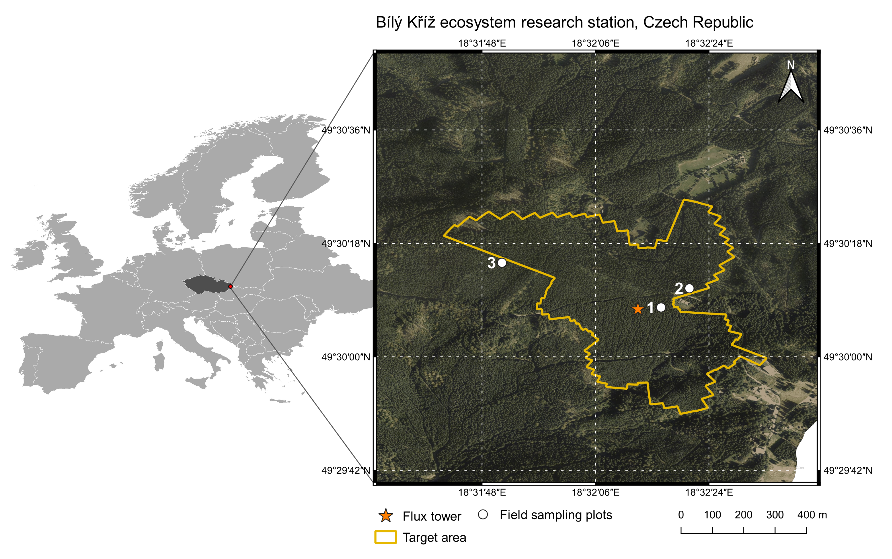
Figure 1. The locations of the eddy covariance flux tower, field sampling plots, and target area defined by the flux footprint at the Bílý Kříž research site.
Remotesensing 12 03773 g001
Figure 2. (a) Temporal variation in mean top-of-canopy (TOC) reflectance in each band extracted from harmonized Landsat-8 and Sentinel-2 (HLS) data within the target area defined by flux footprint (delineated in Figure 1); (b) mean and standard deviation (SD) of TOC reflectance on 31 August 2016 extracted from HLS and airborne data within the target area. The dotted line with triangular symbols is the airborne reflectance resampled to the HLS wavelengths. NIR: near infrared, SWIR: shortwave infrared.
Remotesensing 12 03773 g002
Figure 3. Scatterplot between the observed and simulated top-of-canopy (TOC) reflectance values for each of the 14 days during the 2016 vegetation growing season using the SCOPE radiative transfer module (RTMo). The last plot in the lowermost row shows the result for the airborne data; the other plots show the results for the harmonized Landsat-8 and Sentinel-2 (HLS) data. Values are color-coded by wavelength. The observed TOC reflectance represents the mean reflectance within the target area defined by the flux footprint (delineated in Figure 1). The correlation coefficient (COR) and Nash–Sutchliffe Efficeince (NSE) between observed and simulated TOC reflectance are shown in each plot.
Remotesensing 12 03773 g003
Figure 4. (a–i) Retrieved vegetation properties ( C ab , C w , C dm , C s , C ca , L A I , L I D F , and N); (j) maximum rate of carboxylation ( V cmax ) from the available time series of the harmonized Landsat-8 and Sentinel-2 data during the 2016 growing season. Retrievals from the airborne hyperspectral data for one specific acquisition on 31 August are indicated by the plus sign. Wherever field measurements were available, mean values (diamond sign) and minimum–maximum (Min–Max) ranges are indicated. Information about the vegetation properties is given in Table 2.
Remotesensing 12 03773 g004
Figure 5. Left panels show the daily sum of flux-tower-measured (GPP EC ) and SCOPE-simulated (GPP SIM ) gross primary production for three scenarios: (a,b) Fixed scenario, (c,d) HLS info scenario, and (e,f) HLS info & var Vcmax scenario (detailed in Section 3.3) during the 2016 vegetation growing season. The right panels show the corresponding scatterplots between daily GPP EC and GPP SIM with the statistical evaluations. NSE: Nash–Sutcliffe efficiency, COR: correlation coefficient, RMSE: root mean square error, in g C m−2 s−1).
Remotesensing 12 03773 g005
Figure 6. Dependence of simulated gross primary production (GPP SIM ) within the HLS info scenario on (a) daily mean incoming shortwave radiation (R in ) and (b) daily mean temperature (T a ) during the 2016 vegetation growing season. Values are color-coded by Julian days. Local polynomial regression (loess) was used to show the general trend in the dependencies.
Remotesensing 12 03773 g006
Table 1. Summary statistics of daily (means of half-hourly measurements) meteorological variables during the 2016 vegetation growing season. Min: minimum of daily means, Max: maximum of daily means, Mean: mean of daily means, SD: standard deviation of daily means.
Meteorological VariableSymbolUnitMinMaxMeanSD
Air temperatureT a C −0.6624.6913.775.09
Incoming shortwave radiationR in W / m 2 32.57523.19297.87123.21
Incoming longwave radiationR li W / m 2 258.48391.54328.1227.37
Vapor pressuree a hPa3.4419.4911.503.41
Air pressurephPa895.04925.07914.395.68
Wind speedu m / s 0.776.901.850.97
Table 2. Input parameters for the radiative transfer module (RTMo) of the Soil Canopy Observation of Photosynthesis and Energy fluxes (SCOPE) model together with the lower bound (LB), upper bound (UP), prior mean ( μ ), prior standard deviation (SD), and mean of the measurements acquired in August 2016 from three field sampling plots (Figure 1). The range of the measured soil water content (SWC) in the brightness-shape-moisture (BSM) submodel is provided from Table 3.
ParameterSymbolUnitLBUB μ SDMeasured Mean /Range *
Biochemical propertiesLeaf chlorophyll content C ab μg cm−201005028.838.42
Leaf water content C w g cm−200.050.0250.010.02
Leaf dry matter content C dm g cm−200.040.020.010.015
Senescent material C s 01.50.750.43
Carotenoids C ca μg cm−2020105.777.91
Structural propertiesLeaf area index L A I m2 m−261081.158.66
Leaf inclination distribution function L I D F a –1+100.58
Bimodality of leaf inclination L I D F b –1+100.58
Leaf structural parameterN13.52.250.72
BSM submodel parametersSoil Brightness parameterB00.90.450.26
Soil spectral shape latitude L a t deg10503011.5
Soil spectral shape longitude L o n deg4070558.7
Soil water contentSWC% 15.61–31.54 *
means mean and * means range.
Table 3. Overview of the harmonized Landsat-8 and Sentinel-2 (HLS) data used in this study, with the percentage of high-quality pixels and mean NDVI within the target area defined by flux footprint (delineated in Figure 1). CET: Central European time, NDVI: Normalized difference vegetation index, L30: Landsat-8 data, S30: Sentinel-2 data, SWC: soil water content.
Date of HLS DataSensing SatelliteJulian DayTime of Observation in CET% of High Quality PixelsMean NDVIMean SWC (%) at the Time of Observation
3 April 2016S309411:54:0687.730.7328.45
16 April 2016L3010711:38:1296.470.8231.54
23 May 2016S3014411:54:041000.8123.3
27 May 2016L3014811:32:291000.8424.94
2 July 2016S3018411:52:191000.8718.41
5 July 2016L3018711:38:3078.810.8722.67
22 July 2016S3020411:53:511000.8725.21
31 August 2016L3024411:33:011000.8823.37
7 September 2016L3025111:38:5066.910.8127.23
10 September 2016S3025411:50:2770.450.8723.52
16 September 2016L3026011:33:041000.8817.28
20 September 2016S3026411:52:2399.070.919.31
23 September 2016L3026711:38:511000.8518.95
30 September 2016S3027411:50:2551.860.8615.61
Publisher’s Note: MDPI stays neutral with regard to jurisdictional claims in published maps and institutional affiliations.