Abstract
A Landsat time series has been recognized as a viable source of information for monitoring and assessing forest disturbances and for continuous reporting on forest dynamics. This study focused on developing automated procedures for detecting disturbances in Mediterranean coppice forests which are characterized by rapid regrowth after a cut. Specifically, new methods specific to Mediterranean coppice forests are needed for mapping clearcut disturbances over time and for estimating related indicators in the context of Sustainable Forest Management and Biodiversity International monitoring frameworks. The aim of this work was to develop a new change detection algorithm for mapping clearcut disturbances in Mediterranean coppice forests with Landsat time series (LTS) using a short time window. Accuracy for the new algorithm, characterized as the Two Thresholds Method (TTM), was evaluated using an independent clearcut reference dataset over a temporal period of the 13 years between 2001 and 2013. TTM was also evaluated against two benchmark approaches: (i) LandTrendr, and (ii) the forest loss category of the Global Forest Change Map. Overall Accuracy for LandTrendr and TTM were greater than 0.94. Meanwhile, smaller accuracies were always obtained for the GFC. In particular, Producer’s Accuracy ranged between 0.45 and 0.84 for TTM and between 0.49 and 0.83 for LT, while for the GFC, PA ranged between 0 and 0.38. User’s Accuracy ranged between 0.86 and 0.96 for TTM and between 0.73 and 0.91 for LT, while for the GFC UA ranged between 0.19 and 1.00. Moreover, to illustrate the utility of TTM for mapping clearcut disturbances in Mediterranean coppice forests, we applied TTM to a Landsat scene that covered almost the entirety of the Tuscany region in Italy.
1. Introduction
Sustainable forest management (SFM) is monitored using criteria and indicators [1,2,3,4]. For example, at the international level, the Food and Agriculture Organization of the United Nations (FAO) requires reports of the net annual average change in forest area and the possible reasons for forest loss such as logging activities, natural disturbances, and changes in land use [5]. The Strategic Plan for Biodiversity 2011–2020 approved by the United Nation Convention on Biological Diversity (CBD) provides a long list of indicators that must be assessed to determine if the Aichi Biodiversity Targets are met. These targets were developed to monitor the trends in the implementation of biodiversity strategies across different countries [6]. For example, Aichi Biodiversity Target 5 assesses “the rate of loss of all natural habitats, including forests” through the use of indicators that estimate trends in forest area including trends in forest tree cover and forest area as a percentage of total land area.
At the European level, Forest Europe (formerly the Ministerial Conference on the Protection of Forests in Europe, MCPFE) and the Pan-European Streamlining European Biodiversity Initiative (SEBI) of the European Environmental Agency (EEA) provide a long list of indicators for monitoring the sustainability of forest management and the contribution to nature conservation at country-level [7,8]. Some of these indicators are developed to monitor the temporal trends in forest area, the amount of growing stock volume (GSV), and their changes to understand if forest resources are managed in a sustainable way. In this context, among all the available indicators, those related to the ratio between fellings and increments of forests, both in terms of forest area and GSV, are considered the most important [5,6,7,8]. Estimating the trend in aboveground forest biomass is also crucial for estimating carbon stocks and their fluxes and their relationships with climate change scenarios [9].
SFM indicators are usually estimated using National Forest Inventory (NFI) sample data acquired for reporting aggregated statistics at national or large subnational levels [10,11]. Such statistics are most frequently updated every 5 or 10 years and are based on time-consuming and expensive field surveys [12,13]. White et al. [13] reported that over the entire world, the demand for updated information on forests is increasing, but the trend in financial resources available for traditional forest inventories is decreasing. In response, in the last decades forest inventories have increasingly used remote sensing (RS) technologies to estimate forest parameters in a more cost-efficient way.
Among the vast array of kinds of remotely sensed data, multispectral optical images are still considered the most feasible and cost-effective option for monitoring extensive forest areas [14]. In recent years, multiple approaches for mapping forest dynamics have been developed using time series (TS) of multispectral optical satellite data that are freely available online such as in Landsat, MODIS, and, since 2015, Sentinel-2 data [14,15,16,17,18,19]. The analysis of changes in spectral signatures from TS of satellite images is well-documented as an efficient method for mapping temporal changes in forest environments [18,20]. These methods provide precise estimates of trends in tree cover such as forest loss and gain and can be used to estimate forest indicators needed for international and national SFM monitoring frameworks [20,21,22,23]. For Italy, Puletti et al. [24] developed an automated approach for clearcut detection using Sentinel-2 NDVI spectral trajectory calculated for sample points for a small area. However, this approach cannot reconstruct the history of clearcuts in Italy because Sentinel-2 was only launched in 2015. Landsat time series (LTS), however, are well-suited for monitoring forest dynamics [18,20,23,25] because of their long history. Further, the Landsat mission has contributed to development of a large number of automated methods for detecting forest disturbances over time [19].
The variety of change detection approaches can be divided into two main groups: (i) approaches that use large stacks of image data [26,27,28], and (ii) approaches that use one image per scene per year [29]. Algorithms in the first group require the analysis of large amounts of data but can detect changes over short intervals. Algorithms in this group include the Continuous Change Detection and Classification (CCDC) [26], the Exponentially Weighted Moving Average Change Detection (EWMACD) [28] and the Bayesian Estimator of Abrupt change, Seasonal change, and Trend (BEAST) [30] methods. These methods are promising for detecting forest changes over short temporal intervals such as intra-annual phenological and seasonality changes and forest disturbances. Further, these algorithms have the capability of detecting many kinds and classes of change. However, the dense stacks of image data required by these algorithms make them more difficult to implement by technical operators. Despite the large number of algorithms in this group already developed for monitoring forest by Italian public agencies, nearly all require advanced knowledge of RS [31,32].
Algorithms in the second group require less data, are more suitable for detecting changes between years, and can be easily used by operators. Among the variety of multi-temporal approaches [21] in this group, those using spectral trajectory approaches such as LandTrendr are promising for predicting changes based on the analysis of spectral signatures and facilitate prediction of the post-disturbance vegetation recovery rate. For example, LandTrendr, which uses only one image per year, has been shown to accurately predict forest disturbances in the USA [29,33], Canada [34], Finland [35], and China [36].
Chirici et al. [32] underline how clearcut disturbances in Mediterranean coppice forests can be predicted using trajectories of spectral indices such as Normalized Difference Vegetation Index (NDVI) and Normalized Burned Ratio (NBR) consisting of a single year spike followed by 80% of pixels with disturbances returning to the pre-disturbance conditions after two years. The spectral index spike is the consequence of the rapid regrowth of vegetation after a clearcut in coppice forests and is similar to the spectral behavior that other authors reported as a noise spike due to residual clouds, snow, smoke, or shadows [34,37]. For example, Kennedy et al. [37] asserted that real land cover changes would be more persistent than a single year spike, because for real cover changes the post-spike spectral value does not quickly return to the pre-spike value. These results are not consistent with the spectral behavior of coppice forests in Mediterranean areas as reported by Chirici et al. [32]. In particular, applying spectral trajectory approaches calibrated for boreal and temperate conditions with regrowth rates greater than 10 years [21,23,35,37] to Mediterranean coppice forests would result in disturbances being confused with noise because of the similarity between noise and clearcut spikes. Therefore, tools developed for environmental conditions in boreal and temperate forests [21,23,35,37] may not be suitable for estimating forest indicators using RS data for Mediterranean coppice forests [24].
Coppice forests are a substantial part of the world’s forests representing 83% and 52% in the whole of Europe and at global level, respectively [38,39], with more than 8.5 million hectares in Mediterranean countries [40] where these forests are historically subject to substantial human pressures (i.e., clearcuts with short rotation periods) [41]. However, despite the great importance of coppice forests in Europe for natural and productive purposes [39], especially in Mediterranean countries, there is a lack of continuously updated information on clearcut areas. Currently, the majority of Mediterranean countries report estimates to international organizations such as the FAO and Forest Europe using traditional forest inventory data acquired every 5–10 years [42], at least partially because of the lack of easy-to-use, automated tools specifically designed for Mediterranean environments. In Italy, coppice forests cover more than 3.6 million hectares [43], and Italian coppices account for almost 19% of the coppices in the EU28 [38].
In summary, what is needed for Italian operational use is an algorithm that satisfies the following criteria: (i) use of a TS of Landsat data consisting of a single image per year; (ii) specific calibration for Mediterranean coppice forests using a local dataset; and (iii) automated implementation to facilitate operational use by non-technical, public users. To this end, the aim of the study was to construct such an algorithm. In particular, we developed a new detection algorithm called the Two Thresholds Method (TTM) that is based on a Landsat time series (LTS) of cloud-free imagery for three consecutive years. We compared TTM performance against performances for two benchmark approaches. First, we compared TTM to LandTrendr [35,44], the most widely used spectral trajectory algorithm using one image per year. Second, we compared TTM to the forest loss category of the Global Forest Change Map (GFC) [22], the only global source of forest change data, and the only available forest disturbance map for Italy. To calibrate the method, we used an independent dataset in the form of field a reference clearcut map spanning more than the 13 years from 2000 to 2013 for three study areas in Tuscany. In addition, we used an unbiased stratified estimator to estimate the total clearcut area and the associated standard error for each year.
2. Materials and Methods
2.1. Study Area
The study area consists of 22,987 km2 in Tuscany, Italy, and coincides with the terrestrial portion of Landsat scene 192 030 (Figure 1). The area includes 11,541 km2 of forest and other wood lands [45]. Chirici et al. [46,47] provides a detailed description of forest types and tree species in Tuscany. Forest management is dominated by coppice that is applied in the vast majority of the forested area [32,48]. The area is characterized by a complex landscape with large geographical and topographical variation from flat coastal areas (0 m a.s.l.), to gentle hills, to steep mountains with elevations ranging between 0 and 2000 m a.s.l.
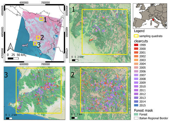
Figure 1.
The upper left panel shows the location of the study area within Landsat scene 192 030 and the locations of the three quadrats. Panels 1, 2, 3 show the locations of clearcuts in the three quadrats of the clearcut reference dataset [32].
A forest mask was constructed using the Copernicus High Resolution Layer tree cover density for the year 2006. We applied a threshold to the tree cover map to obtain a Boolean mask which exactly mimics the official forest area estimate of 11,541 km2 in Tuscany as reported by the last Italian National Forest Inventory [49]. The mask was resampled with a pixel size of 30 m × 30 m to exactly match the geometric resolution of the Landsat imagery. Moreover, because this study is specifically oriented to automated prediction of forest clearcut disturbances, we masked out all the other types of forest disturbance on the forest map. Forest fires were excluded using the national dataset of yearly forest fires officially constructed by the national forest authority using field surveys [50]. Wind damages were reported in Tuscany only for the year 2015 and were excluded on the basis of an available map [46]. Thus, all analyses were conducted only in forest areas free of fire and windthrow damages.
2.2. Landsat Time Series (LTS) Data
The LTS used to develop and test the TTM algorithm was constructed by Chirici et al. [32]. The LTS covered a period of 16 years from 1999 to 2015 and includes one Landsat image per year. To construct the LTS, the image with the least cloud cover (<1%) among the available images acquired during the leaf-on period from May to August was selected for each year.
The images were acquired by three different Landsat sensors: Landsat 5 TM, Landsat 7 ETM+, and Landsat 8 OLI (Table 1). As reported by Chirici et al. [32], the images were processed for cloud and cloud shadow removal and standardized with respect to the spectral response of vegetation with the Ecosystem Disturbance Adaptive Processing System (LE DAPS) [51]. The area covered by clouds and shadows was addressed using a best-pixel-available (BAP) approach designed with a limited phenological window of 30 days around the date of image acquisition [52]. All the LTS images were then masked using the forest/non-forest map, and the resulting images were used as input data for the steps described in the following sections. Chirici et al. [32] provide a complete list of the LTS images used.

Table 1.
Values of the calibration of LandTrendr parameters used to map clearcut forest disturbances.
2.3. Clearcut Reference Dataset
The reference dataset as described in Chirici et al. [32] consists of polygons corresponding to all clearcuts occurring between 1999 and 2015 in three quadrats that were randomly selected along a longitudinal, latitudinal, and altitudinal gradient. Each polygon was designated as clearcut based on photo-interpretation followed by field checking (Figure 1). For each spatial vector polygon, the year of cut disturbance is available (Figure 1).
The clearcut reference dataset was randomly split into (i) calibration and (ii) validation datasets. The calibration dataset consisted of a random selection of 10% of the polygons with 7–10 polygons per year that included approximately 80 ha of the clearcut area per year, or approximately 89,000 Landsat pixels. The dataset was constructed using a quadrat spatial grid (800 m × 800 m) with selection of at most one polygon per grid cell to avoid spatial autocorrelation for each quadrat for each year (Appendix A). This calibration dataset was used to calibrate the TTM and the LandTrendr algorithms. The validation subset consisted of the remaining 90% of the polygons in the clearcut reference dataset for each quadrat for each year and was used to evaluate the accuracies of the TTM, LandTrendr, and GFC methods described in Section 2.5, Section 2.6 and Section 2.7 and to estimate clearcut areas as described in Section 2.9. Thus, the population for which accuracy was assessed and for which clearcut area was estimated consisted of the entire reference dataset less the calibration dataset.
2.4. Raster Grid Validation Datasets
The validation subset was further sub-divided into 13 clearcut polygon datasets, one for each year. Each clearcut polygon dataset was converted to a validation raster grid dataset with the same 30 m × 30 m spatial resolution as the Landsat data and with spatial extent equal to the aggregated area of the three quadrats shown in Figure 1 (i.e., 3 × 225 km2 = 675 km2). The pixels associated with clearcut polygons were classified as “clearcut forest”, while the remaining pixels were classified based on the forest mask (Section 2.2) as either “undisturbed forest” or “non-forest”. Forest pixels associated with clearcut polygons in the calibration dataset were classified as “not considered”. Thus, we obtained 13 raster grid validation datasets that were used to evaluate the accuracy of classifications of forest pixels as either “clearcut forest” or “undisturbed forest”.
2.5. Two Thresholds Method
The Two Thresholds Method (TTM) algorithm uses the LTS and the calibration dataset described in Section 2.4 as input. Optimal values for the TTM parameters are selected using an automated procedure based on the calibration dataset and are used to map forest clearcuts for large areas, typically one or more Landsat scenes. TTM is based on the typical spectral behavior of a clearcut in a coppice system: a rapid decrease in photosynthetic activity immediately following the clearcut and a rapid increase due to vegetative resprouting after 2–3 years. TTM change detection uses a vegetation index such as NDVI or NBR for the vegetative season for three dates: before the cut, immediately following the cut, and a few years after the cut. Based on Chirici et al. [32] we used NBR as the vegetation index calculated as:
where, B4 is the Near Infrared (NIR) Landsat band 4 and B7 is the Short-wave infrared (SWIR) Landsat band 7. TTM predicts forest disturbance at time t, using the NBR vegetation index for three different years NBRt−n, NBRt, NBRt+n. First TTM calculates two differences in NBR (ΔNBR) between times t and t + n as:
ΔNBRpre = NBRt−n − NBRt
ΔNBRpost = NBRt − NBRt+n
Based on preliminary tests, we used the temporal window of t ± 2 years [32]. Using ΔNBRpre and ΔNBRpost, TTM calculates the cumulative percentage histograms for the two ΔNBRs (Figure 2) where npix is the value of the cumulative frequency of all the pixels of ΔNBRs images. On the basis of the two cumulative histograms, TTM repeatedly tests different values of the cumulative frequencies designated npix with values from 0.01 to 1 (Figure 2), to select two cumulative thresholds based on npix (THcut and THregrowth) that identify possible clearcut pixels.
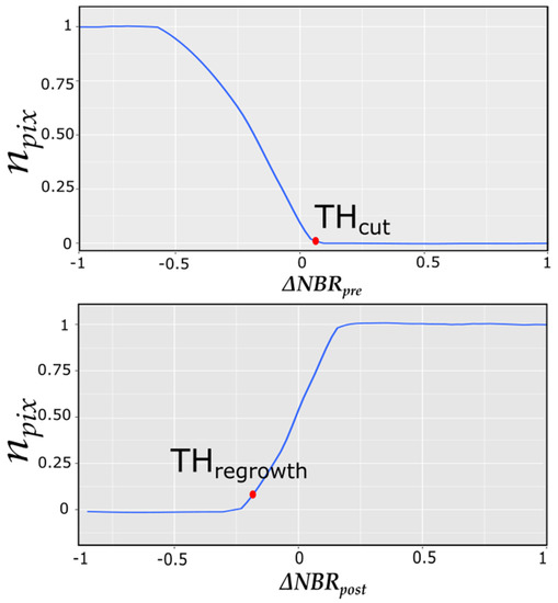
Figure 2.
npix threshold calculated by Two Thresholds Method (TTM) on the basis of cumulative frequency.
In detail, for each value of npix from 0.01 to 1, corresponding values of THcut and THregrowth were selected. Comparing all the possible values, TTM selected two thresholds designated THcut and THregrowth for which and are simultaneously satisfied and classified the pixels as a possible clearcut disturbed pixel. Adjacent clearcut disturbed pixels are then aggregated in vector polygons. TTM assigns to each polygon a fuzzy value of the level of congruency (S) to predict the degree to which and are satisfied as follows:
TTM iteratively tests different thresholds, THs, for S to select only polygons with S < THS.
Each combination of npix and THs produces a different disturbance map. The calibration dataset consisting of 10% of the polygons in the clearcut reference dataset was used with a cross-validation approach to select the optimal values of npix and THs. The validation dataset consisting of the remaining 90% of polygons in the clearcut reference dataset was used as an independent dataset to evaluate the most accurate combination of npix and THs values. The optimal combination of npix and THs was chosen using an accuracy index calculated from the values in a confusion matrix. In particular, we used gmean which is estimated from a confusion matrix as:
where TP is the number of true positives, FP is the number of false positive pixels, FN is the number of false negative pixels and TP is the number of true positive pixels. gmean was used because a small gmean is an indication of poor performance in the classification of the positive cases, even if the negative cases (TN = stable forest) are correctly classified. So, using this index the algorithm avoids overfitting the negative class and under fitting the positive class.
At the end of this calibration procedure, the combination of npix and THs values that produces the greatest accuracy as measured by gmean is applied to the LTS. The resulting spatial polygon dataset includes the year of the clearcut disturbance that is estimated by the automated TTM analysis of spikes in NBR temporal trends as reported by Chirici et al. [32]. The complete TTM scheme can be found in Appendix B. Following the TTM calibration phase, npix = 0.06 and THs = 0.07 were selected as the threshold values that produced the greatest accuracy of gmean = 0.92 (Figure 3).
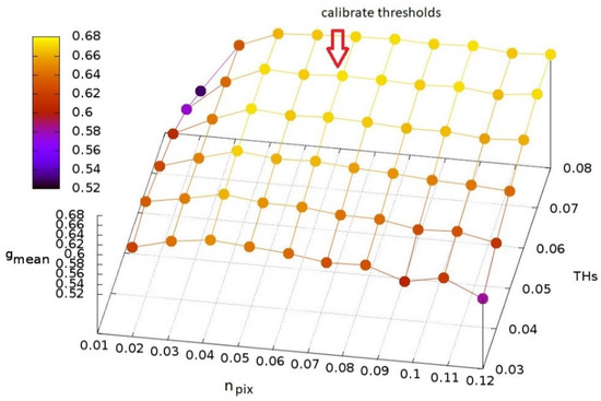
Figure 3.
Calibration of TTM using the calibration dataset in terms of gmean with respect to the parameters npix and THS. The arrow indicates the parameter combination that produced the greatest accuracy.
To evaluate TTM accuracy, the resulting spatial polygon dataset was sub-divided into 13 yearly TTM predicted clearcut datasets, i.e., 2001, …, 2013. Each yearly dataset was converted independently into a raster grid dataset with the same 30 m × 30 m spatial resolution as the Landsat data. For each year, we constructed a TTM raster grid clearcut map for which forest pixels were classified as either “clearcut forest” or “undisturbed forest” using the optimized TTM procedure (Figure 4).
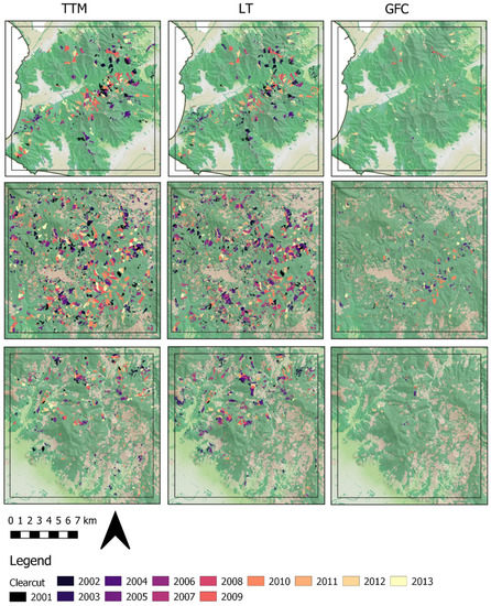
Figure 4.
Clearcut maps estimated using TTM, LandTrendr (LT) and Global Forest Change Map (GFC) for the three areas where the reference validation dataset was available.
2.6. LandTrendr
To further evaluate the TTM algorithm, we compared our results for the three quadrats to those obtained using the well-known LandTrendr algorithm, a trajectory-based method that uses Landsat imagery. We calibrated the algorithm by selecting values for the set of nine LT parameters using the procedure implemented in Google Earth Engine [44]. To obtain comparable LandTrendr results for the years 2000–2013, we had to extend the LTS to the period 1985–2018 because LT-GEE is known to produce large errors for the first and last years if only a short LTS is used [35,44]. As for TTM, the LandTrendr analysis was conducted just in the portion of the study area for forest pixels where no damages related to fire and windstorm were reported; thus, the same forest areas were compared.
The automated features of LT-GEE selected the images and values for the algorithm’s nine parameters that maximized the gmean index using the confusion matrix and the calibration dataset (Table 1). The algorithm with the selected set of parameters was then applied to the LTS. Thirteen raster grid LandTrand clearcut datasets, one for each year, were constructed where each forest pixel was classified as “clearcut forest” or “undisturbed forest” and a year of disturbance was associated with each pixel predicted to have been disturbed (Figure 4).
2.7. Global Forest Change Map (GFC)
The GFC is the only dataset of forest disturbances available for the entire Earth [22]. The GFC map predicts global tree cover extent, loss and gain at a resolution of 30 m × 30 m using TS analyses of more than 655,000 Landsat scenes. Forest loss is defined as stand-replacement disturbance or the complete removal of tree cover canopy at the Landsat pixel scale [22]. The GFC map in Google Earth Engine represents forest change, at 30 m × 30 m resolution, globally, between 2000 and 2018 and is available at https://earthenginepartners.appspot.com/science-2013-global-forest.
We downloaded the GFC disturbance map for the study areas for the years 2000–2013, applied the forest mask, and clipped the map to the areas of the three quadrats. As for the TTM and LandTrendr, we omitted from the GFC analysis pixels for which fires and windstorms were officially reported. We constructed 13 GFC clearcut raster grid datasets, one per year, with forest pixels classified as either “clearcut forest” or “undisturbed forest” (Figure 4).
2.8. Accuracy Assessment
The accuracies of the pixel-level “undisturbed forest” or “clearcut forest” classifications for the three quadrats were estimated using the validation dataset for each of the three methods and each year (i.e., the 13 TTM clearcut raster grid datasets, the 13 GFC clearcut raster grid datasets and the 13 LandTrendr clearcut datasets) based on 2 × 2 confusion matrices constructed using the 13 independent validation raster grid datasets available for the three quadrats (Figure 2). For each confusion matrix, we calculated TP, TN, FP, and FN, the gmean index as reported in Equation (6), the overall accuracy, the sensitivity, the precision, producer’s accuracy, and user’s accuracy calculated as:
2.9. Clearcut Area Estimates
To comply with Aichi Biodiversity Target 5, SEBI, and Forest Europe reporting requirements regarding loss of natural forests, we estimated clearcut areas using maps of the three quadrats constructed using the optimized TTM for each of the 13 years. An intuitive approach for estimating the areas would be simply to add the areas of all map units classified as clearcut, i.e., . Estimates obtained with this approach are denoted map estimates. However, this approach, often characterized as pixel counting, is biased because it does not account for map classification error.
An unbiased stratified estimator based on the entries in a confusion matrix constructed using the optimized TTM-base map and reference data was used to estimate clearcut areas (Table 2). With this estimator, the clearcut area is estimated as,
with standard error,
where Atot is the total area (i.e., forest area of the three quadrats 8898.21 ha) which is assumed to be without error, w1 is the proportion of the total area in the “clearcut forest” map class, and w2 is the proportion of the total area in the “undisturbed forest” map class. Three reference sets were used with the stratified estimator. Firstly, all pixels in the entire validation dataset described in Section 2.4 were used as a reference data for constructing the confusion matrix and estimating the clearcut areas. Because this reference set consisted of exactly the same pixels as the population for which clearcut area was estimated (Section 2.4), this analysis comprises a census of the population. Further, because the reference set size, n, equals the population size, N, then in the variance estimator shown in Table 2 with the result that the estimates, designated as the “census” estimates, are exact without uncertainty, i.e., . Secondly, we used a random selection of 50% of the pixels in the validation data described in Section 2.4 as the reference set for constructing a second confusion matrix with the resulting area estimates designated as the “large sample” estimates. Thirdly, because obtaining a large reference set is very laborious and time-consuming, estimates were also calculated using a much smaller reference dataset. This reference set was constructed using a square 1500 m × 1500 m grid covering the validation dataset with a point randomly selected from within each cell formed by the grid lines. The resulting area estimates were designed as the “point sample” estimates. The stratified estimator is unbiased when used with random samples, meaning that over all possible samples of the same size, the mean of the sample-based estimates equals the true value. However, even with an unbiased estimator, the estimate for any particular sample may still deviate substantially from the true value. The standard error and associated confidence interval provide a measure of this potential deviation.
Table 2.
Confusion matrix (Nh in the last column is the total number of map units in the hth map class).
3. Results
3.1. Accuacy Assessment
The maps constructed for the three quadrats with the three methods are presented in Figure 4.
We estimated accuracies for the three quadrats using all the confusion matrix validation indices for each method and each year using the 13 raster grid validation datasets (Figure 5). Overall, accuracies for TTM and LandTrendr were much greater than for the GFC, particularly for 2001–2011. Accuracies were comparable for TTM and LandTrendr, albeit slightly greater for TTM (Figure 5, Appendix C, and Appendix D). All accuracies for LandTrendr and TTM were greater than 0.94. Similar results were found for Specificity, Precision, Producer’s (PA) and User’s accuracy (UA) for “clearcut forest” with TTM and LandTrendr producing comparable results, while smaller estimates were always obtained for the GFC (Figure 5). In particular, PA ranged between 0.45 and 0.84 for TTM and between 0.49 and 0.83 for LT, while for the GFC, PA ranged between 0 and 0.38. UA ranged between 0.86 and 0.96 for TTM and between 0.73 and 0.91 for LT, while for the GFC UA ranged between 0.19 and 1.00.
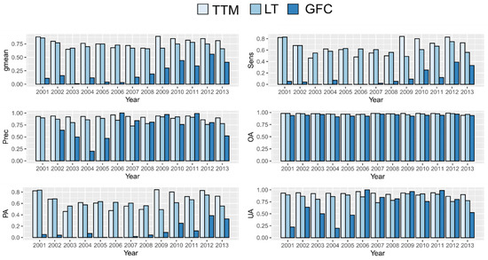
Figure 5.
Accuracy estimates based on confusion matrices constructed using the validation dataset for the three quadrats. The vertical axis represents the accuracy indices (gmean = gmean accuracy index, Sen = sensitivity, Prec = precision, OA = Overall Accuracy, PA = Producer Accuracy of clearcut class, UA = Users Accuracy of clearcut class).
LandTrendr and TTM produced comparable overall accuracies, but for 10 of the 13 years, TTM produced greater accuracies with 0.65 ≤ gmean ≤ 0.89 than LandTrendr with 0.66 ≤ gmean ≤ 0.78. The average gmean for TTM over the 13 years was 0.78 versus 0.72 for LandTrendr. Further, TTM produced accurate results for year of disturbance t after two additional years, whereas LandTrendr required at least three additional years. gmean accuracies for the GFC [22] over the 13 years were much smaller than for the other methods, ranging between 0.07 and 0.56. The GFC also had many omission errors relative to the other two methods (Figure 5).
3.2. Area Estimation
3.2.1. The Three Quadrats
The census, large sample, and point sample estimates of clearcut areas for the three quadrats are reported in Table 3. The similarity between the estimates is as expected because the map accuracies are large, and the stratified estimator is unbiased for these analyses.
Table 3.
Clearcut (CC) area estimates (census estimates based on entire validation dataset; small sample estimates based on 50% random sample of the validation dataset; point sample estimates based on photointerpretation of 200 randomly selected points).
3.2.2. Large Scale Clearcut Mapping and Area Estimation
Because TTM produced the greatest accuracies for the three quadrats, we applied it to the entirety of Landsat scene 192 030 within the borders of the administrative Region of Tuscany. We used the same parameters selected during the calibration phase (t ± 2 years, npix = 0.06 and THS = 0.07), and estimated statistics for forest harvesting from 2000 to 2013. For the 13 years, the map indicated 73,819 ha of forest, representing 14.21% of the total forest area (Figure 6).
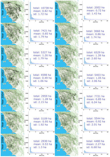
Figure 6.
Final clearcuts maps obtained with the TTM algorithm and related frequency histograms of sizes of clearcut areas within the portion of Landsat scene 192 030 within the borders of Tuscany Region.
We estimated that the clearcut area per year in the portion of Landsat scene 192 030 within the borders of Tuscany Region was less than 2% of the total forest area (Figure 7). Although these map-based (pixel counting) estimates are subject to uncertainty due to map classification error, the large map accuracies reported in Table 2 suggest that such uncertainties are likely small.
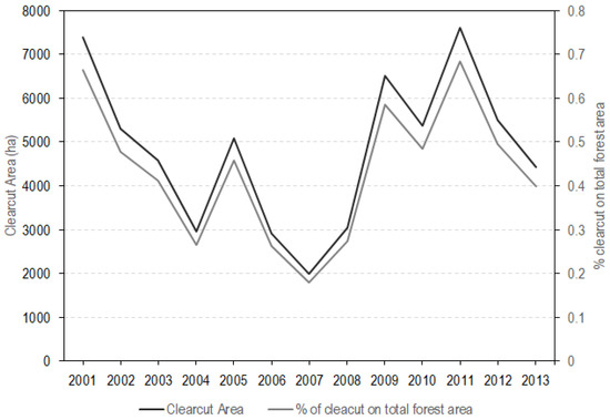
Figure 7.
Yearly clearcut area (line black—first vertical axis) and percentages of forest area logged (grey line—second vertical axis) in the portion of Landsat scene 192 030 within the borders of Tuscany Region.
TTM predicted 81,915 forest cuts of which the vast majority (79%) were between 0.5 and 2.0 ha (Figure 8). Small clearcuts represented 18,559.8 ha or 25% of the total forest cut area as predicted by TTM in the study period.
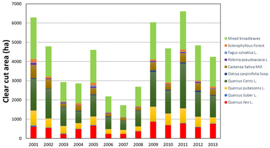
Figure 8.
Forest area logged by year and for the main Tuscany forest types in the portion of Landsat scene 192 030 within the borders of Tuscany Region.
We analyzed cuts by forest types using the vegetation map produced by Arrigoni for the Tuscany region [53]. Of the total clearcut areas, 34% was in mixed broadleaves forest (Figure 8), 29% was in Quercus cerris L. forest, 12% was in Quercus ilex L. forest, 11% was in Quercus pubescens L. forest, and 8% was in Castanea sativa Mill. forest (Figure 8).
4. Discussion
4.1. The Algorithm
This study, to the best of our knowledge, is the first effort to develop an automated procedure that uses Landsat TS data to map clearcuts in Mediterranean forest areas that are managed with the coppice system. We found that a 3-year temporal analysis of the spectral vegetation trajectories was a logical procedure for predicting these types of disturbances because the spectral trajectories of Mediterranean clearcuts are characterized by spikes of t − 2, t and t + 2. Specifically, 3 years after a clearcut, coppice vegetation indices are similar to indices observed before the clearcut. In fact, if we calculate the ΔNBR before 3 (t − 1) and after 3 years (t + 3) the differences will be close to zero in which case TTM would not predict a clearcut. For the same reason, the algorithm does not predict the same clearcut in two consecutive years because the NBR spectral trajectory for Mediterranean coppices reflects the rapid regrowth. Potentially, the same procedure can be also applied to other types of forest ecosystems characterized by rapid regrowth, such as tropical forests, that have spectral trajectories similar to those of Mediterranean coppice forests [54]. TTM required calibration using a small set of manually mapped clearcuts to facilitate automated optimal selection of the two thresholds used by the TTM (npix and THs). Because the values of the two TTM thresholds did not change for different years for the same Landsat scene, we expect that values for these threshold parameters may be valid across multiple Landsat images as long as the selected vegetation index, NBR in our case, is calculated using normalized images such as those we produced with the LEDAPS procedure. TTM was implemented using the NBR vegetation index with a time window of t ± 2 years where t is the year when the clearcut occurs. We found that five years (t − 2, t, t + 2) are needed to detect clearcuts, because inaccurate results were found using smaller time windows. Perhaps the time needed to detect clearcuts in coppices forests can be reduced by the algorithms developed for intra-annual change detection such as CCD [26], EWMACD [28], and BEAST [30]. However, at the moment, the use of these types of algorithms require an advanced knowledge of RS that is a limitation to application by technical operators from Italian public agencies. Moreover, TTM produced accurate spatially continuous maps of harvested areas just two years after the clearcut which is consistent with our intent and with the Italian regulation (Figure 6). Moreover, the data required to calibrate the algorithm (i.e., 7–10 polygons) are already available in the public forest authority datasets, because they are collected during the clearcut authorization procedure. Moreover, these maps can be used by local or national forest authorities to estimate some of the most common indicators requested by international agreements, such as the ratio between increments and loggings [5,6,8] without the need for expensive field activities [13]. From an international perspective, TTM may be limited because it is specifically designed for Mediterranean coppice forests characterized by rapid regrowth after logging. However, for clearcut monitoring in Italy, TTM is a valid approach, because large clearcuts in Italy are permitted only in coppice forests.
4.2. Accuracy Assessment
TTM produced results comparable to results for the well-known LandTrendr [35,37,45] and to the results of a previous study by Puletti et al. [34] using Sentinel-2 data. However, the LandTrendr calibration procedure for forests for this study differed relative to calibration for temperate and boreal forests. Firstly, to use LandTrendr in Mediterranean conditions, an accurate forest mask is needed; otherwise the specific parametrization may result in commission errors due to spectral behavior in agricultural lands. For temperate and boreal forests, a forest mask may not be necessary [37,44]. Secondly, the Recovery threshold value for the LandTrandr algorithm for Mediterranean conditions is 0.55, while a value of approximately 0.30 was sufficient for other forest types [37,44].
The LandTrendr calibration procedure was time-consuming and required considerable imagery to produce accurate results [37]. To detect clearcuts at time t, TTM required just three images (t − 2, t, t + 2) spanning a period of five years, whereas LandTrendr required at least 10 images spanning a period of at least 10 years between t − 5 and t + 5. In fact, for TTM we obtained accurate forest clearcut maps for the period 2000–2013 with a LTS covering a period of 16 years (1999–2015), whereas LandTrendr required a longer LTS with images covering a period of 33 years (1985–2018) [35]. Therefore, in this study, we found that TTM can accurately predict clearcuts at time t at least three years before LandTrendr.
We found that both TTM and LandTrendr produced more accurate results than the GFC [22]. This result was not unexpected, because the GFC is constructed using an automated approach developed to provide statistics for forest disturbances at a global scale. TTM and LandTrendr were, instead, specifically calibrated for the study area. Thus, the GFC cannot be considered a valid source of information for producing forest disturbance statistics in Italy. It is important to remember that different automated algorithms can be useful for mapping different land/forest changes or disturbances. However, each algorithm must be evaluated to understand its strengths and weaknesses in terms of omission and commission error rates and with respect to the target change/disturbance [55]. In our, case we observed that TTM and LT have fewer omission and commission errors than the GFC. We found that beginning with 2009, both the TTM and LT algorithms produced large values of gmean compared to values for the years 2003–2008. This result can be partially explained by analyzing climate conditions between the years used to detect the clearcuts. For example, for 2009 we found that the climate conditions between 2007 and 2011 (i.e., t ± 2) were similar, so the reflectance of the images used were not affected by reflection due to drought. In fact, for example, we found that independently of the methods used, accuracies were smallest for the year 2003. A possible explanation is that 2003 was one of the driest years in the last two decades in Italy. The drought caused a rapid decline in all vegetation types. All three methods were characterized by greater commission error rates as a result of the negative spectral spikes caused by local, strong, drought-induced decreases in NBR which may be confused with the similar spectral behavior of logged areas.
4.3. Area Estimation
Finally, although motivation for the study did not necessarily include support for greenhouse gas (GHG) inventories, it merits noting that the combination of the mapping approach and the sample-based stratified clearcut area estimator complies with the good practice guidelines of the Intergovernmental Panel on Climate Change: (1) “neither over- nor underestimates so far as can be judged,” and (3) “uncertainties are reduced as far as practicable” [56]. For the large sample for some of the years, we obtained . The phenomenon is attributed to the combination of large accuracies and a very large sample size for variance estimation. For the points sample with a small sample size, less than about 1% of the population size, 1-n/N can be ignored so that usually does not occur (Table 3).
5. Conclusions
The following conclusions can be drawn from the study:
- TTM is the first algorithm specifically developed for Mediterranean conditions using Landsat TS to predict forest clearcuts in coppice forests that can be used for constructing accurate spatially explicit maps of forest harvesting areas and for operationally estimating sustainable forest management indicators in the framework of international agreements;
- TTM was easy to use, and its configuration is adjustable using a calibration dataset. TTM can be used for mapping and continuous reporting on forest clearcut disturbances in Mediterranean forests;
- LandTrendr for Mediterranean forests requires an accurate forest mask, otherwise the specific parametrization may result in commission errors due to spectral confusion with agricultural lands;
- The GFC substantially underestimates the area of clearcut disturbances in Mediterranean coppice forests.
Future research efforts should focus on two issues: (i) testing TTM with different optical satellite time series such as Sentinel-2 images, and (ii) mapping forest disturbances in other Mediterranean forests, for example, in continuous cover forestry.
Author Contributions
Conceptualization, G.C.; methodology, R.P.; writing—review and editing F.G., G.C., D.T., R.E.M., S.F.; M.M., G.S.M.; data curation, R.P., S.F., writing—original draft F.G. All authors have read and agreed to the published version of the manuscript.
Funding
This research received no external funding.
Acknowledgments
We wish to thank Erika Mazza for her help in the construction of the reference dataset, and we are grateful to three anonymous reviewers and the Editor who contributed to improving the original version of the manuscript with their suggestions and comments.
Conflicts of Interest
The authors declare no conflict of interest.
Appendix A. Example of Calibration Dataset for 2010

Appendix B. Workflow Scheme of TTM Functionality

Appendix C. TP, TN, FN, FP of Clercut Forest Classes

Appendix D. Producer’s and Users’ Accuracy of “Not Disturbed Forests” for the Three Methods
| TTM | LT | GFC | ||||
| Year | PA | UA | PA | UA | PA | UA |
| 2001 | 1.00 | 0.94 | 0.99 | 0.94 | 0.99 | 1.00 |
| 2002 | 1.00 | 0.96 | 0.99 | 0.96 | 1.00 | 1.00 |
| 2003 | 1.00 | 0.98 | 0.99 | 0.98 | 1.00 | 1.00 |
| 2004 | 1.00 | 0.95 | 0.99 | 0.96 | 0.98 | 0.99 |
| 2005 | 1.00 | 0.95 | 0.99 | 0.95 | 1.00 | 1.00 |
| 2006 | 1.00 | 0.96 | 0.99 | 0.95 | 1.00 | 1.00 |
| 2007 | 1.00 | 0.98 | 0.99 | 0.98 | 1.00 | 1.00 |
| 2008 | 1.00 | 0.98 | 0.99 | 0.97 | 1.00 | 1.00 |
| 2009 | 0.99 | 0.93 | 1.00 | 0.96 | 1.00 | 0.99 |
| 2010 | 0.99 | 0.94 | 1.00 | 0.96 | 0.99 | 0.98 |
| 2011 | 1.00 | 0.95 | 1.00 | 0.96 | 1.00 | 0.99 |
| 2012 | 0.99 | 0.96 | 0.99 | 0.96 | 1.00 | 0.98 |
| 2013 | 0.99 | 0.95 | 0.99 | 0.96 | 0.98 | 0.98 |
References
- Barbati, A.; Marchetti, M.; Chirici, G.; Corona, P. European Forest Types and Forest Europe SFM indicators: Tools for monitoring progress on forest biodiversity conservation. For. Ecol. Manag. 2014, 321, 145–157. [Google Scholar] [CrossRef]
- Galluzzi, M.; Giannetti, F.; Puletti, N.; Canullo, R.; Rocchini, D.; Bastrup, A.; Gherardo, B. A plot–level exploratory analysis of European forest based on the results from the BioSoil Forest Biodiversity project. Eur. J. For. Res. 2019. [Google Scholar] [CrossRef]
- Fotakis, D.G.; Sidiropoulos, E.; Myronidis, D.; Ioannou, K. Spatial genetic algorithm for multi-objective forest planning. For. Policy Econ. 2012, 21, 12–19. [Google Scholar] [CrossRef]
- Chirici, G.; McRoberts, R.E.; Winter, S.; Bertini, R.; Bröändli, U.-B.; Asensio, I.A.; Bastrup-Birk, A.; Rondeux, J.; Barsoum, N.; Marchetti, M. National forest inventory contributions to forest biodiversity monitoring. For. Sci. 2012, 58, 257–268. [Google Scholar] [CrossRef]
- FAO. State of the World’s Forests 2016. In Forests and Agriculture: Land-Use Challenges and Opportunities; FAO: Rome, Italy, 2016; Volume 45. [Google Scholar]
- Conservation on Biological Diversity (CBD). Indicators for the Strategic Plan for Biodiversity 2011–2020 and the Aichi Biodiversity Targets. Available online: https://www.cbd.int/doc/strategic-plan/strategic-plan-indicators-en.pdf 2016 (accessed on 9 November 2020).
- European Environment Agency Streamlining European Biodiversity Indicators 2020: Building a Future on Lessons Learnt from the SEBI 2010 Process; European Environment Agency: Copenhagen, Denmark, 2012.
- FOREST EUROPE. State of Europe’s Forests 2015; Ministerial Conference on the Protection of Forests in Europe FOREST EUROPE Liaison Unit Madrid: Madrid, Spain, 2015; Available online: https://www.foresteurope.org/docs/fullsoef2015.pdf (accessed on 9 November 2020).
- IPCC. 2006 IPCC Guidelines for National Greenhouse Gas Inventories; Eggleston, H.S., Buendia, L., Miwa, K., Ngara, T., Tanabe, K., Eds.; Prepared by the National Greenhouse Gas Inventories Programme; IGES: Geneva, Switzerland, 2006. [Google Scholar]
- Kangas, A.; Maltamo, M. Forest Inventory. Methodology and Application; Springer: Berlin, Germany, 2006; ISBN 9781402043819. [Google Scholar]
- Macdicken, K.G. Forest Ecology and Management Global Forest Resources Assessment 2015: What, why and how? For. Ecol. Manag. 2015, 352, 3–8. [Google Scholar] [CrossRef]
- Tomppo, E.; Katila, M.; Mäkisara, K.; Peräsaari, J. The Multi-Source National Forest Inventory of Finland—Methods and Results 2007. In Multi-Source National Forest Inventory; Managing Forest Ecosystems; Springer: Dordrecht, The Netherlands, 2008; Volume 18. [Google Scholar]
- White, J.C.; Coops, N.C.; Wulder, M.A.; Vastaranta, M.; Hilker, T.; Tompalski, P.; White, J.C.; Coops, N.C.; Wulder, M.A.; Vastaranta, M.; et al. Remote Sensing Technologies for Enhancing Forest Inventories: A Review. Can. J. Remote Sens. 2016, 42, 619–641. [Google Scholar] [CrossRef]
- Gómez, C.; White, J.C.; Wulder, M.A. ISPRS Journal of Photogrammetry and Remote Sensing Optical remotely sensed time series data for land cover classification: A review. ISPRS J. Photogramm. Remote Sens. 2016, 116, 55–72. [Google Scholar] [CrossRef]
- Zhang, H.K.; Roy, D.P. Using the 500 m MODIS land cover product to derive a consistent continental scale 30 m Landsat land cover classi fi cation. Remote Sens. Environ. 2017, 197, 15–34. [Google Scholar] [CrossRef]
- Banskota, A.; Kayastha, N.; Falkowski, M.J.; Wulder, M.A.; Froese, R.E.; White, J.C.; Banskota, A.; Kayastha, N.; Falkowski, M.J.; Michael, A.; et al. Forest Monitoring Using Landsat Time Series Data: A Review. Can. J. Remote Sens. 2014, 8992, 362–384. [Google Scholar] [CrossRef]
- Fragoso-campón, L.; Quirós, E.; Mora, J.; Gutiérrez, J.A.; Durán-barroso, P. Accuracy Enhancement for Land Cover Classification Using LiDAR and Multitemporal Sentinel 2 Images in a Forested Watershed. Proceedings 2018, 2, 1280. [Google Scholar] [CrossRef]
- Gómez, C.; White, J.C.; Wulder, M.A. Characterizing the state and processes of change in a dynamic forest environment using hierarchical spatio-temporal segmentation. Remote Sens. Environ. 2011, 115, 1665–1679. [Google Scholar] [CrossRef]
- Wulder, M.A.; Loveland, T.R.; Roy, D.P.; Crawford, C.J.; Masek, G.; Woodcock, C.E.; Allen, R.G.; Anderson, M.C.; Belward, A.S.; Cohen, W.B.; et al. Current status of Landsat program, science, and applications. Remote Sens. Environ. 2019, 225, 127–147. [Google Scholar] [CrossRef]
- Wulder, M.A.; White, J.C.; Goward, S.N.; Masek, J.G.; Irons, J.R.; Herold, M.; Cohen, W.B.; Loveland, T.R.; Woodcock, C.E. Landsat continuity: Issues and opportunities for land cover monitoring. Remote Sens. Environ. 2008, 112, 955–969. [Google Scholar] [CrossRef]
- White, J.C.; Saarinen, N.; Wulder, M.A.; Kankare, V.; Hermosilla, T.; Coops, N.C.; Holopainen, M.; Hyyppä, J.; Vastaranta, M.; Service, C.F.; et al. Assessing spectral measures of post-harvest forest recovery with field plot data. Int. J. Appl. Earth Obs. Geoinf. 2019, 80, 102–114. [Google Scholar] [CrossRef]
- Hansen, M.C.; Potapov, P.V.; Moore, R.; Hancher, M.; Turubanova, S.A.; Tyukavina, A. High-Resolution Global Maps of 21st-Century Forest Cover Change. Science 2013, 342, 850–854. [Google Scholar] [CrossRef]
- Matasci, G.; Hermosilla, T.; Wulder, M.A.; White, J.C.; Coops, N.C.; Hobart, G.W.; Zald, H.S.J. Large-area mapping of Canadian boreal forest cover, height, biomass and other structural attributes using Landsat composites and lidar plots. Remote Sens. Environ. 2018, 209, 90–106. [Google Scholar] [CrossRef]
- Puletti, N.; Bascietto, M. Towards a tool for early detection and estimation of forest cuttings by remotely sensed data. Land 2019, 8, 58. [Google Scholar] [CrossRef]
- Bonney, M.T.; Danby, R.K.; Treitz, P.M. Landscape variability of vegetation change across the forest to tundra transition of central Canada. Remote Sens. Environ. 2018, 217, 18–29. [Google Scholar] [CrossRef]
- Zhu, Z.; Woodcock, C.E. Continuous change detection and classification of land cover using all available Landsat data. Remote Sens. Environ. 2014, 144, 152–171. [Google Scholar] [CrossRef]
- Cai, S.; Liu, D. Detecting change dates from dense satellite time series using a sub-annual change detection algorithm. Remote Sens. 2015, 7, 8705–8727. [Google Scholar] [CrossRef]
- Brooks, E.B.; Yang, Z.; Thomas, V.A.; Wynne, R.H. Edyn: Dynamic signaling of changes to forests using exponentially weighted moving average charts. Forests 2017, 8, 304. [Google Scholar] [CrossRef]
- Zhu, Z. Change detection using landsat time series: A review of frequencies, preprocessing, algorithms, and applications. ISPRS J. Photogramm. Remote Sens. 2017, 130, 370–384. [Google Scholar] [CrossRef]
- Zhao, K.; Wulder, M.A.; Hu, T.; Bright, R.; Wu, Q.; Qin, H.; Li, Y.; Toman, E.; Mallick, B.; Zhang, X.; et al. Detecting change-point, trend, and seasonality in satellite time series data to track abrupt changes and nonlinear dynamics: A Bayesian ensemble algorithm. Remote Sens. Environ. 2019, 232, 111181. [Google Scholar] [CrossRef]
- Scarascia-Mugnozza, G.; Oswald, H.; Piussi, P.; Radoglou, K. Forests of the Mediterranean region: Gaps in knowledge and research needs. For. Ecol. Manage. 2000, 132, 97–109. [Google Scholar] [CrossRef]
- Chirici, G.; Giannetti, F.; Mazza, E.; Francini, S.; Travaglini, D.; Pegna, R.; White, J.C. Monitoring clearcutting and subsequent rapid recovery in Mediterranean coppice forests with Landsat time series. Ann. For. Sci. 2020, 77, 40. [Google Scholar] [CrossRef]
- Cohen, W.B.; Yang, Z.; Kennedy, R. Detecting trends in forest disturbance and recovery using yearly Landsat time series: 2. TimeSync—Tools for calibration and validation. Remote Sens. Environ. 2010, 114, 2911–2924. [Google Scholar] [CrossRef]
- White, J.C.; Saarinen, N.; Kankare, V.; Wulder, M.A.; Hermosilla, T. Confirmation of post-harvest spectral recovery from Landsat time series using measures of forest cover and height derived from airborne laser scanning data. Remote Sens. Environ. 2018, 216, 262–275. [Google Scholar] [CrossRef]
- Cohen, W.B.; Yang, Z.; Healey, S.P.; Kennedy, R.E.; Gorelick, N. A LandTrendr multispectral ensemble for forest disturbance detection. Remote Sens. Environ. 2018, 205, 131–140. [Google Scholar] [CrossRef]
- Tang, D.; Fan, H.; Yang, K.; Zhang, Y. Mapping forest disturbance across the China–Laos border using annual Landsat time series. Int. J. Remote Sens. 2019, 40, 2895–2915. [Google Scholar] [CrossRef]
- Kennedy, R.E.; Yang, Z.; Cohen, W.B. Detecting trends in forest disturbance and recovery using yearly Landsat time series: 1. LandTrendr—Temporal segmentation algorithms. Remote Sens. Environ. 2010, 114, 2897–2910. [Google Scholar] [CrossRef]
- Fabbio, G. Coppice forests, or the changeable aspect of things, a review. Ann. Silvic. Res. 2016, 40, 108–132. [Google Scholar] [CrossRef]
- Mairota, P.; Buckley, P.; Suchomel, C.; Heinsoo, K.; Verheyen, K.; Hédl, R.; Terzuolo, P.G.; Sindaco, R.; Carpanelli, A. Integrating conservation objectives into forest management: Coppice management and forest habitats in Natura 2000 sites. IForest 2016, 9, 560–568. [Google Scholar] [CrossRef]
- Morandini, R. Improvement of coppice forests in the Mediterranean region. In Procindigs of the Workshop Improvement of Coppice Forest in Mediterranean Region; Istituto Sperimentale per la Selvicoltrura: Arezzo, Italy, 1994. [Google Scholar]
- FAO and Plan Bleu. State of Mediterranean Forests 2018; FAO: Rome, Italy, 2018; ISBN 978-92-5-131047-2. [Google Scholar]
- FAO. Strategic framework on mediterranean forests. In Proceedings of the High Level Segment Third Mediterranean Forest Week, Tlemcen, Algeria, 21 March 2013. [Google Scholar]
- Tabacchi, G.; Di Cosmo, L.; Gasparini, P.; Morelli, S. Stima del Volume e della Fitomassa delle Principali Specie Forestali Italiene, Equazioni di Previsione, Tavole del Volume e Tavole della Fitomassa Arborea Epigea; Consiglio per la Ricerca e la Sperimentazione in Agricoltura, Unità di Ricerca per il Monitoraggio e la Pianificazione Forestale: Trento, Italy, 2011; ISBN 9788897081111. [Google Scholar]
- Kennedy, R.E.; Yang, Z.; Gorelick, N.; Cohen, W.B.; Healey, S. Implementation of the LandTrendr Algorithm on Google Earth Engine. Remote Sens. 2018, 10, 691. [Google Scholar] [CrossRef]
- Borghetti, M.; Chirici, G. Raw data from the Italian National Forest Inventory are on-line and publicly available. For. Riv. Selvic. Ecol. For. 2016, 13, 33–34. [Google Scholar] [CrossRef]
- Chirici, G.; Bottalico, F.; Giannetti, F.; Del Perugia, B.; Travaglini, D.; Nocentini, S.; Kutchartt, E.; Marchi, E.; Foderi, C.; Fioravanti, M.; et al. Assessing forest windthrow damage using single-date, post-event airborne laser scanning data. For. Int. J. For. Res. 2018, 1, 27–37. [Google Scholar] [CrossRef]
- Chirici, G.; Giannetti, F.; McRoberts, R.E.; Travaglini, D.; Pecchi, M.; Maselli, F.; Chiesi, M.; Corona, P. Wall-to-wall spatial prediction of growing stock volume based on Italian National Forest Inventory plots and remotely sensed data. Int. J. Appl. Earth Obs. Geoinf. 2020, 84, 101959. [Google Scholar] [CrossRef]
- Bottalico, F.; Travaglini, D.; Chirici, G.; Marchetti, M.; Marchi, E.; Nocentini, S.; Corona, P. Classifying silvicultural systems (coppices vs. high forests) in mediterranean oak forests by airborne laser scanning data. Eur. J. Remote Sens. 2014, 47, 437–460. [Google Scholar] [CrossRef]
- INFC Il disegno di Campionamento. Inventario Nazionale delle Foreste e dei Serbatoi Forestali di Carbonio; MiPAF—Direzione Generale per le Risorse Forestali Montane e Idriche, Corpo Forestale dello Stato, ISAFA: Trento, Italy; 36p, Available online: http://www.isafa.it/scientifica/2004 (accessed on 7 November 2020).
- Arma dei Carabinieri—Comando Unità per la Tutela Forestale Ambientale e Agroalimentare. Catasto Incendi. In Ufficio Logistico—2^ Sezione Sistemi Informativi Automatizzati e TLC; via Carducci 5—00187; Arma dei Carabinieri—Comando Unità per la Tutela Forestale Ambientale e Agroalimentare: Roma, Italy, 2018. [Google Scholar]
- Masek, J.G.; Vermote, E.F.; Saleous, N.; Wolfe, R.; Hall, F.G.; Huemmrich, F.; Gao, F.; Kutler, J.; Lim, T.K. LEDAPS Calibration, Reflectance, Atmospheric Correction Preprocessing Code, Version 2; ORNL DAAC: Oak Ridge, TE, USA, 2013. [Google Scholar] [CrossRef]
- White, J.C.; Wulder, M.A.; Hobart, G.W.; Luther, J.E.; Hermosilla, T.; Griffiths, P.; Coops, N.C.; Hall, R.J.; Hostert, P.; Dyk, A.; et al. Pixel-based image compositing for large-area dense time series applications and science. Can. J. Remote Sens. 2014, 40, 192–212. [Google Scholar] [CrossRef]
- Arrigoni, P.V.; Raffaelli, M.; Rizzotto, M.; Selvi, F.; Foggi, B.; Viciani, D.; Lombardi, L.; Benesperi, R.; Ferretti, G.; Benucci, S.; et al. Carta Della Vegetazione Forestale Della Regione Toscana. Scala 1:250.000; SELCA, Firenze Editor, Regione Toscana, Giunta Regionale: Firenze, Italy, 1999. [Google Scholar]
- Wang, Y.; Ziv, G.; Adami, M.; Mitchard, E.; Batterman, S.A.; Buermann, W.; Schwantes Marimon, B.; Marimon Junior, B.H.; Matias Reis, S.; Rodrigues, D.; et al. Mapping tropical disturbed forests using multi-decadal 30 m optical satellite imagery. Remote Sens. Environ. 2019, 221, 474–488. [Google Scholar] [CrossRef]
- Cohen, W.B.; Healey, S.P.; Yang, Z.; Stehman, S.V.; Brewer, C.K.; Brooks, E.B.; Gorelick, N.; Huang, C.; Hughes, M.J.; Kennedy, R.E.; et al. How Similar Are Forest Disturbance Maps Derived from Different Landsat Time Series Algorithms? Forests 2017, 8, 98. [Google Scholar] [CrossRef]
- Eggleston, H.S.; Buendia, L.; Miwa, K.; Ngara, T.; Tanabe, K. (Eds.) IPCC Guidelines for National Greenhouse Gas Inventories, Volume 4: Agriculture, Forestry and Other Land Use; Institute for Global Environmental Strategies: Hayama, Japan, 2006; Available online: http://www.ipcc-nggip.iges.or.jp/public/2006gl/index.html (accessed on 9 November 2020).
Publisher’s Note: MDPI stays neutral with regard to jurisdictional claims in published maps and institutional affiliations. |
© 2020 by the authors. Licensee MDPI, Basel, Switzerland. This article is an open access article distributed under the terms and conditions of the Creative Commons Attribution (CC BY) license (http://creativecommons.org/licenses/by/4.0/).