Conductor Reconstruction for Dynamic Line Rating Using Vehicle-Mounted LiDAR

Abstract

Dynamic Line Rating (DLR) is a process which electrical network operators can implement to improve efficiency by dynamically adjusting the load capacity as conditions allow. To implement DLR an accurate model of the conductors and their clearances is needed. Airborne LiDAR, while expensive, is the most common method of collecting line data as it is fast and is of high quality. State of the art methods for automatically reconstructing conductors first classify conductor points before fitting conductor models. This approach works well for high tension lines with significant separation between conductors but tends to perform poorly in urban environments where conductors are packed tightly together and surrounded by clutter. The method presented in this article attempts to overcome these challenges by performing an informed search for the conductors, anchored to the utility poles. Before the conductors are classified, their layout and sag are estimated, converting conductor segmentation into a linear problem; and a 3D to 2D projection is used to improve density and simplify clustering. The work also attempts to reduce the cost of conductor reconstruction by utilising lower-cost vehicle-mounted LiDAR. By avoiding point classification, higher precision can be achieved in scenarios where previous methods have suffered from significantly degraded performance.

1. Introduction

Within an electrical network each circuit has a static rating which states the maximum capacity under normal operating conditions. These current ratings are constrained by either safety codes which restrict the maximum amount of conductor sag due to thermal expansion before a clearance violation occurs [1], or the point at which the conductor will begin to anneal, causing permanent damage [2]. A line rating is first calculated when the circuit is installed, but only adjusted infrequently afterwards. Dynamic Line Rating (DLR) is a paradigm shift which allows for line ratings to be dynamically updated in real time as environmental conditions change. The process of implementing DLR requires that the clearance between the conductors and nearby objects be accurately surveyed. There are tools available to assist in measuring conductor clearances (laser and acoustic range finders [3,4]), but this task remains time consuming and labour intensive. Alternatively, airborne LiDAR can be used to rapidly survey large amounts of electrical infrastructure [5], albeit at significant cost.

The development of smaller and cheaper LiDAR units has increased interest in performing surveys using vehicle-mounted LiDAR. The reduced survey cost has moved the challenge for transmission network operators from acquiring data, to having efficient means of analysis.

Our work is focused on the reconstruction of road side electrical conductors contained within 3D scans of urban environments collected using vehicle mounted LiDAR. The aim is to provide accurate 3D models of the electrical infrastructure within the scan which can then be used to derive the metrics required to implement and maintain DLR. The main contributions of the presented work includes: (1) a method of clustering conductors which is robust to portions of the conductor being unobserved; (2) reconstruction of conductors where their configuration is unknown; (3) and a comparison with a current state of the art conductor recovery method.

2. Related Work

The automated reconstruction of power-line spans is not new to the field of remote sensing. Much of the focus has been on reconstructing high tension spans from LiDAR data collected from aircraft [6,7,8,9,10,11]. These methods show some common patterns. With the application of voxel-based, density-based, and location-based filters the majority of non-conductor points are removed from the scan. Afterwards, conductor primitives are assigned to the conductor like regions; these regions are usually identified by comparing the magnitude of the three eigenvalues describing the local point distribution. A region growing algorithm may then be used to cluster these primitives into larger groups before either RANSAC or least squares is used to fit a conductor model.

One reason that the bulk of conductor recovery research has been focused on high tension spans is these have large inter-conductor distances and more clearance from the ground and other objects in the scan. In spans where conductors are packed closely it is challenging to calculate eigenvalues for a single conductor. The method proposed by Jwa et al. worked around this issue by using the Hough Transform first to recover the cardinal direction of the conductors [12].

It is uncommon for conductor recovery methods to first recover the power-poles or pylons to constrain the conductor search. However, as pointed out by Guo et al, locating the pylons first is helpful for power line reconstruction [13]. Guo used the JointBoost classifier to identify regions of the point cloud likely belonging to high tension pylons. Between these pylons, a structured search was conducted which identified conductor primitives.

Cheng et al [14] developed one of the few methods for reconstructing power lines using vehicle-mounted LiDAR. Like many of the other conductor recovery methods, Cheng used a bottom-up approach, first applying filters, then reconstructing the conductors from more primitive segments. Unlike previous methods, Cheng’s method needed to be more robust to segments of the conductors being unobserved due to obstruction from other objects; something that is uncommon in scans collected from aircraft. Fortunately for Cheng, while portions of the conductors were obscured from view, the conductors were well separated from each other allowing for the computation of eigenvalues for individual conductors; a feature that was used for the reconstruction.

The most common approach used to recover conductors is to start by first identifying small regions of the point cloud which are conductor-like. These conductor-like primitives are then used to reconstruct the entire conductor span. Building a robust system to define these conductor primitives is key to the performance of the rest of the recovery process; and is not a trivial task. The conductor recovery method proposed by Liang et al. overcame this challenge by requiring the conductor region to be manually delineated [15], while Wang et al. used an SVM to filter non-conductor points based on local features [16].

Some methods make use of a Digital Elevation Model (DEM) [6,14,17] to develop point features; including that proposed by Liang et al. Liang used the height of a point above the DEM along with the LiDAR return information as features to classify conductor points. This method measures the distance between the first and second return in aerial LiDAR. For returns that are separated by large distances, it is likely that the first return may be from a conductor, as conductors generally have a large amount of vertical clearance from the ground below. However, if the returns are closely packed then the object is more likely to be the canopy of a tree. It is important to note that methods that make use of the relationships between multiple returns are likely to be heavily dependent on the sensor’s perspective, i.e methods for airborne LiDAR would be less effective on datasets collected from vehicle-mounted LiDAR.

The most common method of point classification is based on the local point distribution [7,12,13,14,17]. One challenge that occurs when classifying points based on the local distribution, is handling when the conductors are close together. The method proposed by Mclaughlin et al. made use of an ellipsoid shaped window aligned with the flight path to reduce the probability that multiple conductors would pollute the feature generation [11].

Each of the methods discussed above build up conductor primitives using locally derived features. By applying filters over various scales, points belonging to conductors can be preserved, while non-conductor points are suppressed. However, these methods still result in some non-conductor points being falsely classified as belonging to conductors. The method proposed by Guo et al. attempts to reduce the frequency of these false positives by building a structural understanding of the scan [13]. By first identifying the pylons, not only can the conductor search space be reduced, but the conductor orientation can also be inferred. This knowledge regarding the conductor configuration is incorporated into the subsequent steps of conductor reconstruction.

The ultimate objective of all conductor recovery methods is to assign a parametric model to the span. These models all assume that each span is confined to a single vertical plane [11]; i.e., the conductor is hanging directly down and not at an angle as if blown by the wind. One of two different models is then used to describe the shape of the conductor on the plane, otherwise referred to as the conductor sag. While the physically accurate model to describe a hanging conductor is the catenary, a parabolic model is often substituted as the catenary equation uses a transcendental function which can make model fitting more difficult [6,15]. At the scale and tension conductors are expected to be under, the use of a parabolic model over a catenary model is considered an acceptable compromise [14].

3. Method

Our proposed conductor recovery method is comprised of seven sequential steps. (1) First utility poles are located within the scan. (2) These poles are used to define the conductor search space. (3) Next the number of conductor levels is determined and (4) the sag for each level is removed from the conductor points. (5) These de-sagged conductor points are projected onto a clustering plane and (6) the individual conductors within each level are clustered. (7) Finally a conductor model is fitted to the clustered conductors.

3.1. Pole Localisation

Point clouds generated from vehicle mounted LiDAR can contain many strings of points as each of the lasers sweep through the scene. Filtering the strings can prove difficult as they can bare resemblance to the conductors within the scene [18]. Instead of using local features to filter out non-conductor points, the search for conductors is constrained to only between utility poles. The utility poles are recovered from the point cloud using a method proposed by McCulloch and Green [19,20]. This pole recovery method searches for pole cross-sections within horizontal slices of the original point cloud. Poles are then reconstructed by stitching together pole cross-sections which are aligned vertically. This method was selected because it is able to robustly recover both the pole’s base and top when the pole’s structure is partially occluded by surrounding clutter; a condition that is often present in vehicle based scans.

3.2. Conductor Search Space

A conductor search space is a cuboid region located between two poles. For every pair of poles less than 40 m apart a conductor search space is defined. The poles are located at either end of the region and define its length. The width of the region is three meters and it extends vertically to include all points within the footprint. As the region is aligned with the two poles at either end, any conductors fixed to the two poles will also be closely aligned with the major axis of the conductor search space.

3.3. Conductor Level Determination

Conductors within a single span are divided up into discrete levels; conductors on the same level are attached to a common cross-arm at each pole. Any span between two connected poles will have one or more conductor levels. Accurately determining the number of conductor levels is critical to the subsequent conductor reconstruction operations.

The proposed method for determining the configuration of conductor levels uses a process where the conductor search space is divided into sub-regions. To construct these sub regions the conductor search space is first divided along the span-wise direction into regions referred to as windows. Each of these windows extends 2.5 m along the span. A window size of 2.5 m is small enough to allow for many independent estimations of the conductor level configuration along the span, and also that the conductors contained within it do not exhibit a significant amount of vertical travel. While large enough to ensure that a conductor is well represented within the window.

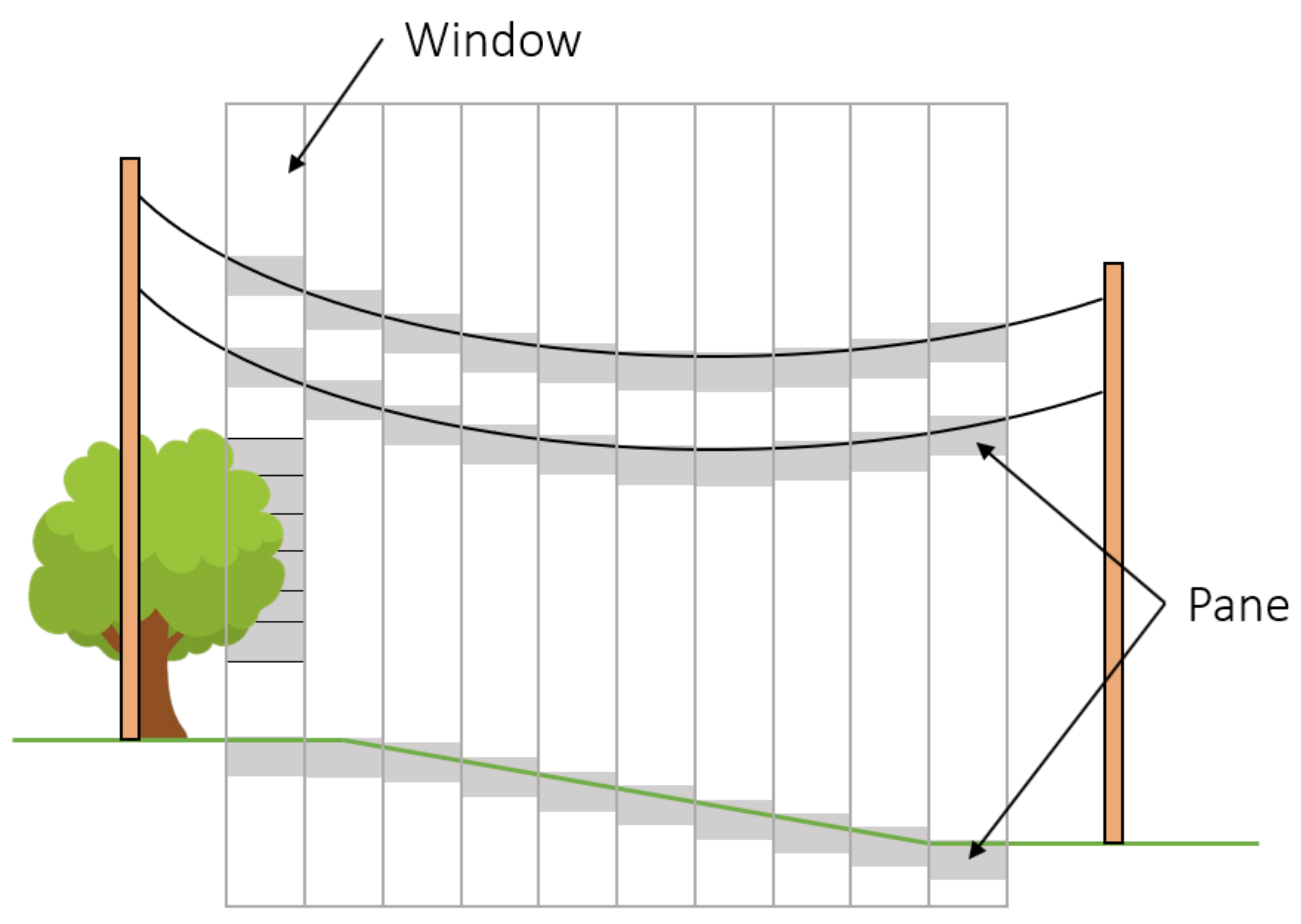
Each window is then further subdivided into regions referred to as panes. Panes are used to resolve discrete regions within the window where objects exist. The process of generating a window’s panes starts with the upper most point within the window. This uppermost point defines the top of the first pane. The bottom of this first pane is 0.5 m below the top. Starting at the bottom of the previous pane, the next highest point within the window is used to seed the top of the next pane. This process continues until all points within the window are also included within a pane; see Figure 1.

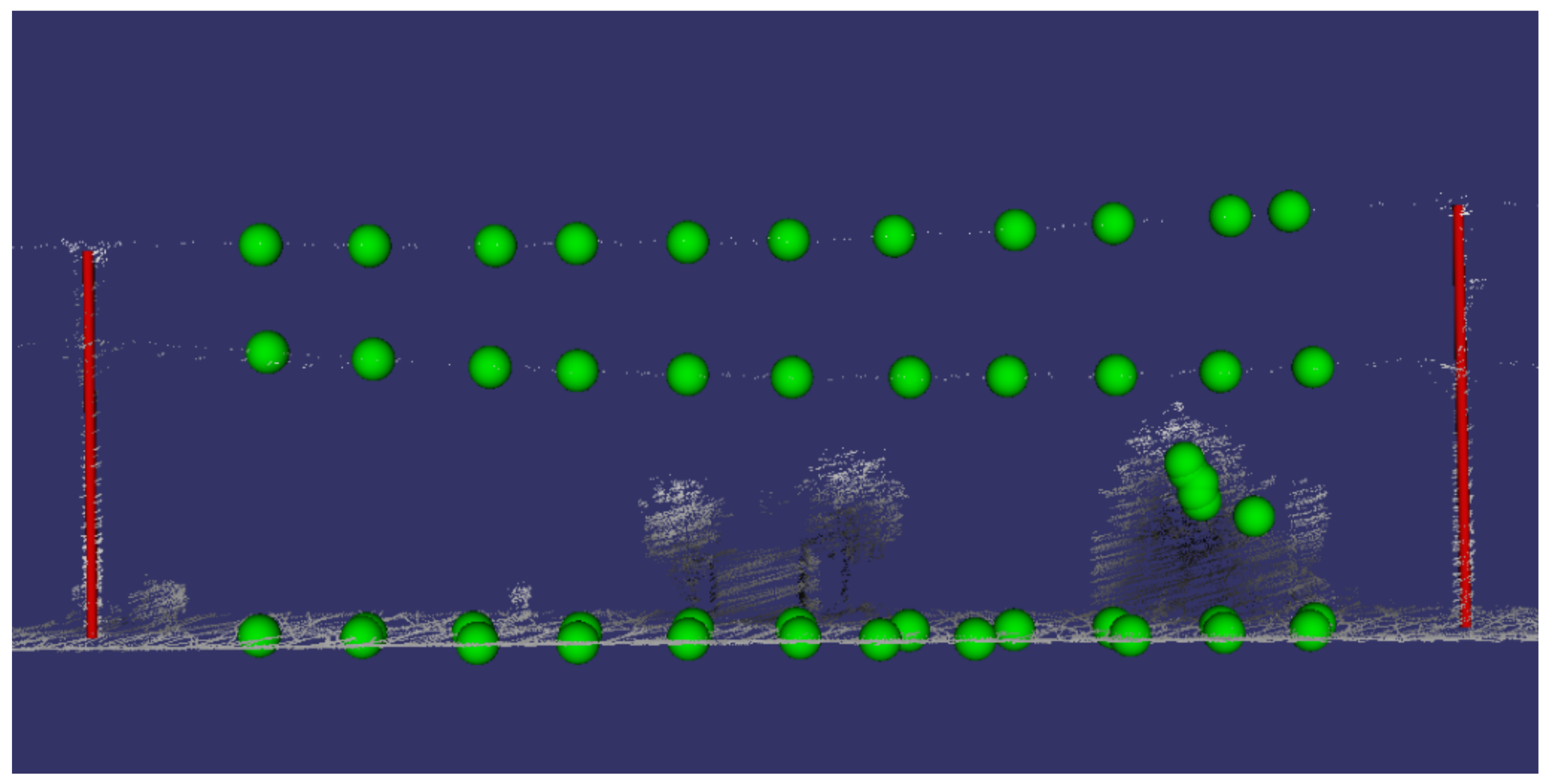
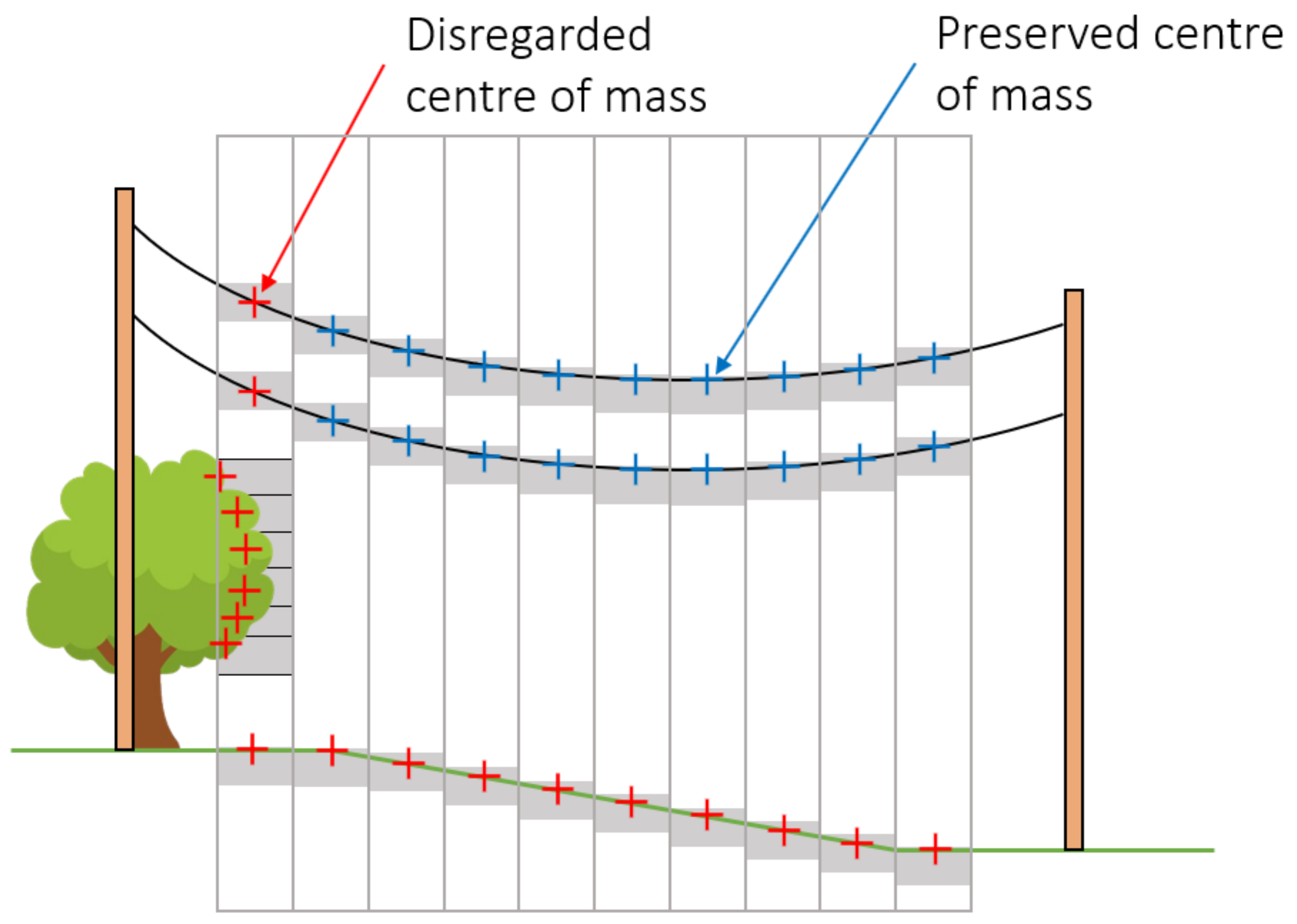
The centre of mass (COM) for the points contained within each pane is then computed; see Figure 2. Two filters are used to remove COMs belonging to regions other than those representing conductors. The first filter removes COMs without enough vertical clearance between itself an its neighbours within the same window. This filter removes the COMs generated by vertical structures such as trees and other ground clutter. As conductors are thin and do not fall by more than 0.5 m within a single window, they are not removed by this filter. The second filter removes any centre of masses less than 1 m above the vector linking the two pole bottoms. This filter is designed to remove points along the ground. This is required because often the ground will have less than 0.5 m in height difference within a single window. With such a small variance in height, the ground will occupy a single pane and result in only one centre of mass. Figure 3 illustrates these filtering processes.

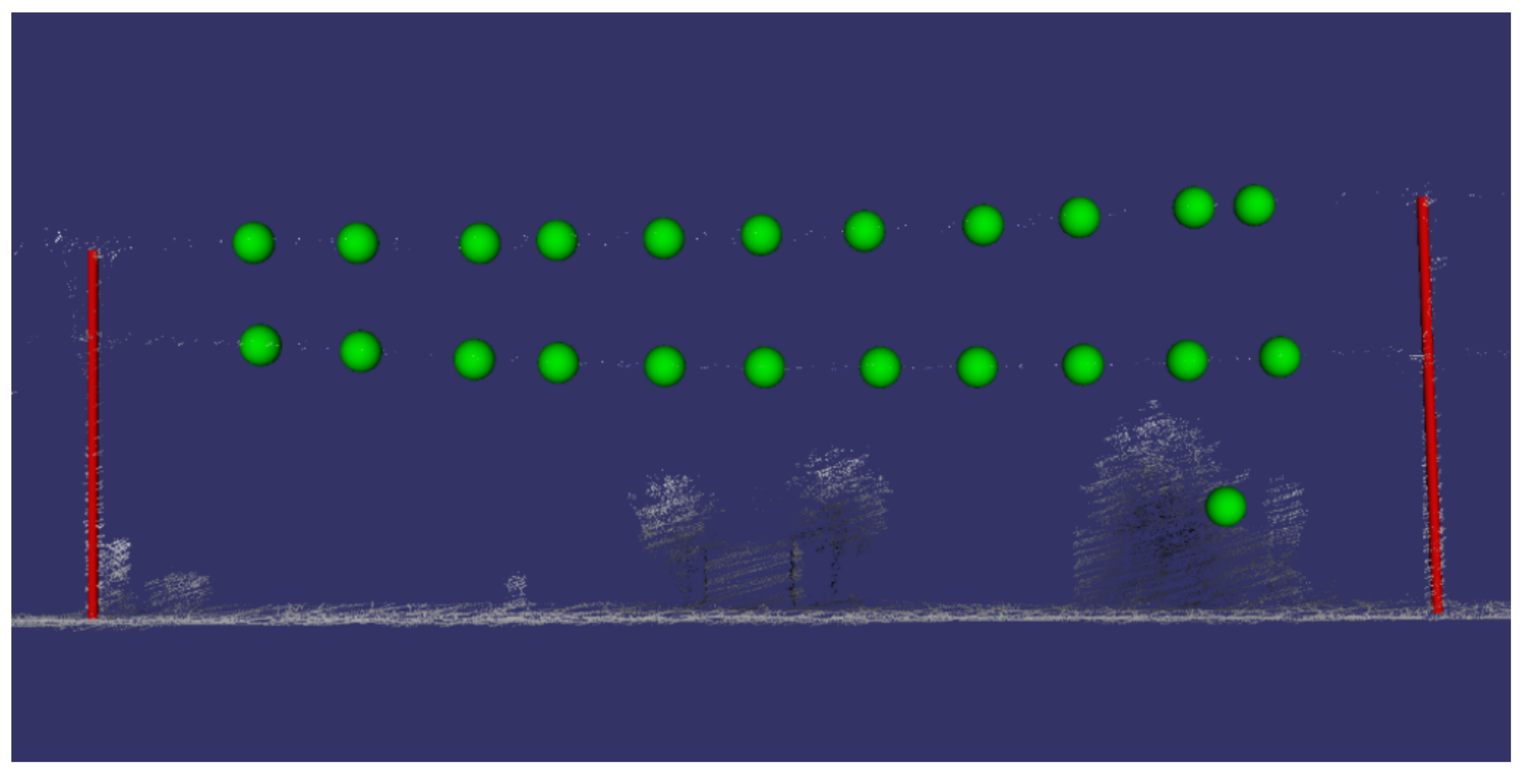
The modal number of remaining COMs within each window is used to calculate the number of conductor levels. The mode allows for the number of conductor levels to be robustly calculated in situations where erroneous COMs have survived the filtering process; see Figure 4.

3.4. Conductor Sag Compensation

A conductor sag model is generated for each of the conductor levels using the filtered set of COMs. The COMs are grouped based on their vertical order within the windows, i.e. all of the topmost centre of masses are grouped together. Any window with an incorrect number of COMs is not included within this process.

Each collection of COMs within the vertical stack is then used to fit a conductor sag model. This process fits a 2-dimensional catenary to the vertical and span-wise components of the COMs using a least-squares solver [21]. An example of fitted sag models can be seen in Figure 5. Three tests are applied to check the validity of the fitted sag models. (1) The model is checked that is is hanging downwards, (2) that the model’s ground clearance is more that 2.5 m, (3) and that the conductor model does not terminate more than 1 m above the connected pole tops. The sag model is allowed to terminate above the pole top to allow for the extra height provided by the cross-arm and insulators. The thresholds for these criteria have been selected with wide tolerances, this is to ensure that models are not falsely rejected. When models are generated falsely, they tend to be significantly incorrect, and thus still rejected using these thresholds.

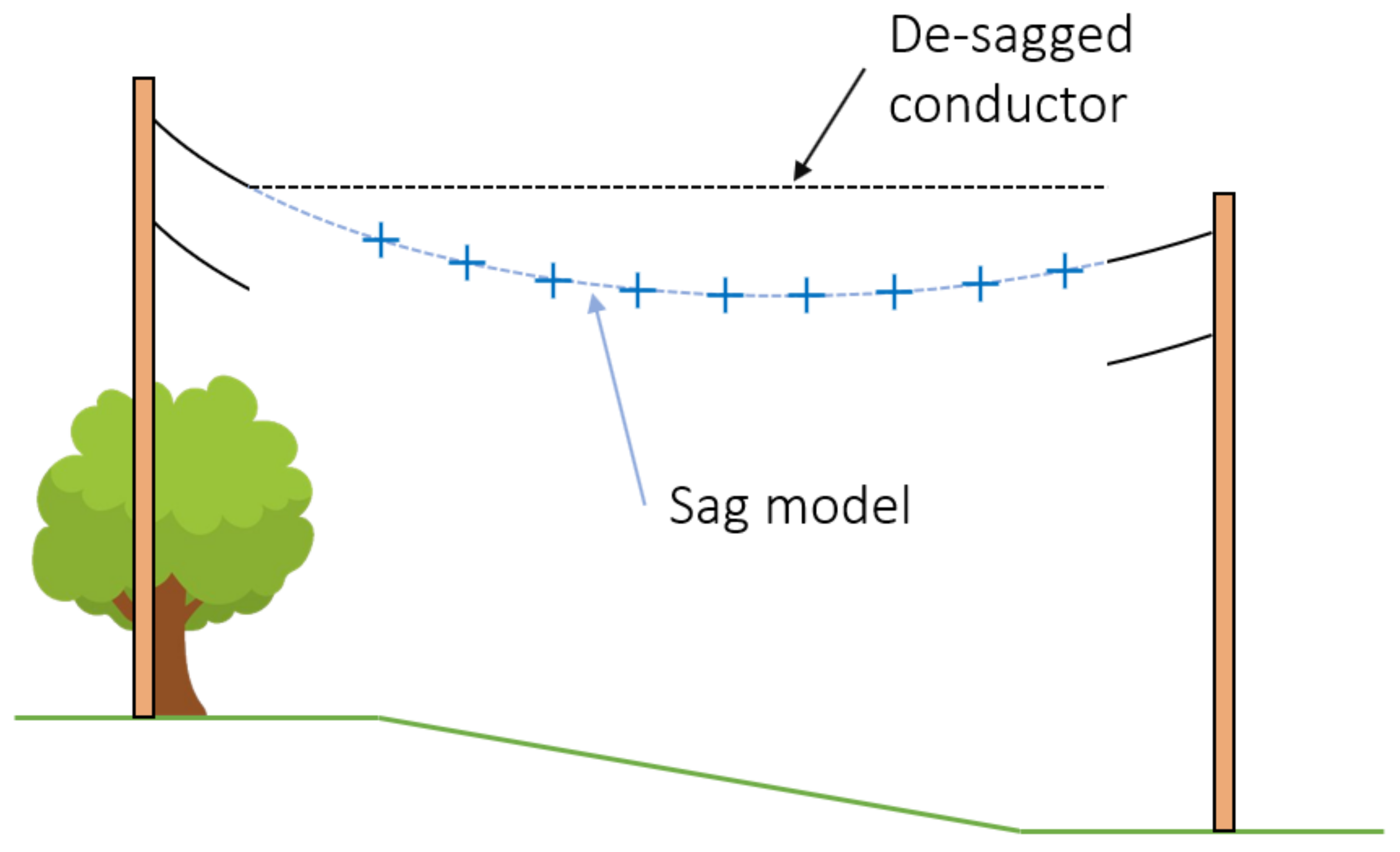
All points within the conductor search space are then filtered using these conductor level sag models. If a point is less the 0.25 m vertically from a conductor sag model, it is associated with the conductor level, otherwise it is discarded. This results in a set of points for each conductor level. The points within each conductor level set then have their sag removed by subtracting the estimated sag computed using the same conductor level sag model used to segment them; See Figure 6.

3.5. Clustering Plane

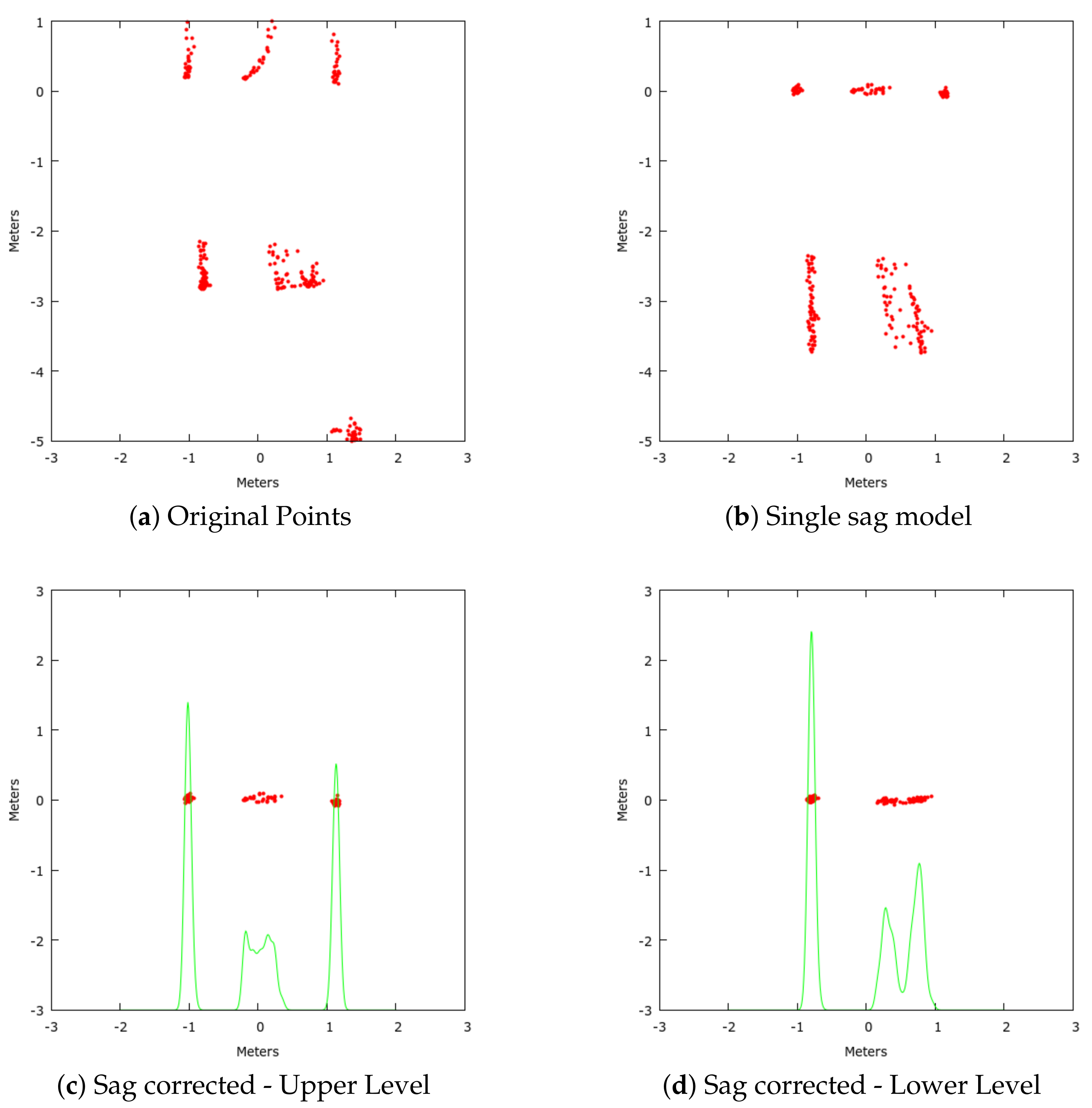
The clustering plane is a projection technique previously introduced [18] to improve point density and simplify the clustering processes. The clustering plane is a plane perpendicular to the span-wise direction. Points within the conductor search space are projected onto this plane by removing their span-wise component; see examples in Figure 7. In this previous work, points were directly projected onto the clustering plane which resulted in them appearing as vertical structures due to the conductors’ hanging shape. This previous work also had no notion of conductor levels, thus all points were projected onto the same plane; increasing the clustering complexity. Our new proposed method can overcome both of these limitations by leveraging the conductor sag models. Each conductor level is processed individually and a separate clustering plane is used for each one. Because these points have had their sag removed in the previous step, they appear in tight groupings; a significant improvement compared to the vertical structures that the previous work suffered from.

3.6. Conductor Clustering

Conductor clustering is performed on the 2-Dimensional points in the clustering plane. In previous work this clustering process was made more complex by multiple conductor levels being projected onto the same plane, and the vertical distortion caused by the hanging shape of the conductors. Clustering using this sag compensation method is considerably easier as conductors form tighter clusters with significantly less distortion. Three clustering algorithms were considered, K-Means, DBSCAN, and Mean-shift. K-Means was ruled out because determining the number of conductors on a given level can be challenging. DBSCAN was ruled out because the density of conductor clusters varies a lot based on many factors including conductor diameter, age, length of span, and distance from the LiDAR. Ultimately Mean-shift clustering was selected because, while we may not know the number and density of conductors, the shape and size of conductors on the clustering plane is fairly consistent regardless of the conductors’ parameters. Following clustering, each cluster is tested to ensure the points within it are distributed along the entire span. This test is used to eliminate clusters formed by other structures close to the target conductors and present on the clustering plane, such as other conductors not belonging to this span but sharing one of the poles. This test is performed by dividing the conductor search space into thirds along the span-wise direction and discarding any clusters which do not have points present in each region.

3.7. Conductor Model Fitting

Conductor models consist of two components. The horizontal component describes the cross span-wise offset (point along the cross-arm where the conductor is attached). The horizontal component is found using the cross-spanwise component of the cluster on the clustering plane. The vertical component describes the height of the conductor for any given point along the span and is based on the cantenary model. The vertical component is fitted to the original 3-Dimensional points which made up the projected cluster on the clustering plane. This fitting process is similar to the conductor level sag model fitting process described in Section 3.4. As with sag model fitting, the fitted conductor model also undergoes the same three tests to identify and eliminate erroneous models. These tests being that the conductor is hanging downward, there is more than 2.5 m clearance with the ground, and that the conductor does not terminate more than 1 m above the pole tops.

4. Test Cases

4.1. Mapping Data

The proposed algorithm was tested on datasets captured using a vehicle-mounted mobile laser scanner. The system is based around a single Velodyne VLP-16; a LiDAR with a spatial accuracy of $\pm 3$ cm [22]. This LiDAR is mounted to the roof of a vehicle at the height of 1.6 m and a downward inclination of 10 degrees in the forward direction. The downward inclination allows LiDAR to both scan points ahead and behind the vehicle while also increasing the number of intersections with the overhead conductors. The raw range data from the LiDAR is collected using an embedded Linux computer for later reconstruction. A point cloud is generated from the raw range data after collection is complete using the LiDAR Odometry And Mapping (LOAM) algorithm [23]. This reconstruction takes place on a workstation with significantly more computing resources than available to the data collection computer attached to the LiDAR.

The conductors within a scan are divided up into three categories; primary, secondary, and road-crossing. A conductor is part of the primary group if it is a candidate for DLR; this is the case if it is part of the main circuit for that street. Secondary conductors are conductors that are not being considered for DLR; they are used for feeding individual houses and do not carry enough current to warrant the implementation of DLR. In these scans the conductors which are crossing roads are also not part of the primary circuit, instead they are used for feeding small groups of houses on the opposite side of the road to the primary circuit. We have separated the road crossing conductors from the other secondary conductors, because they are not as well observed or represented due to being largely orthogonal to the path taken by the scanner.

4.2. Hounslow Dataset

The point cloud for the Hounslow dataset was collected along a 240 m narrow stretch of road in a well-established suburban area of Christchurch City, New Zealand. The data was collected by driving the length of the test area, completing a U-Turn at an intersection, and observing the test area again by driving in the opposite direction. The Hounslow dataset contains 24 primary conductors contained within six spans running along one side of the street. A fifth communications cable is present in these spans, but disregarded due to its irrelevance to the application of this research. There are three conductors crossing the road and three secondary conductors on the opposite side of the road. All of these conductors are suspended from 13 poles. Many of the conductors in this dataset have less than one meter of horizontal separation from trees alongside.

4.3. Gilberthorpes Dataset

The point cloud for the Gilberthorpes dataset was collected along a 680 m stretch on the outskirts of Christchurch City, New Zealand. The spans tested in this dataset stretch between 19 poles along the western side of the street. These spans have two layers of conductors, most commonly with three conductors on the upper level and five on the lower. In addition to these primary conductors there are 8 secondary conductors on the opposite side of the road to the vehicles path and 19 crossing over the road.

4.4. Comparison with Previous Works’ Datasets

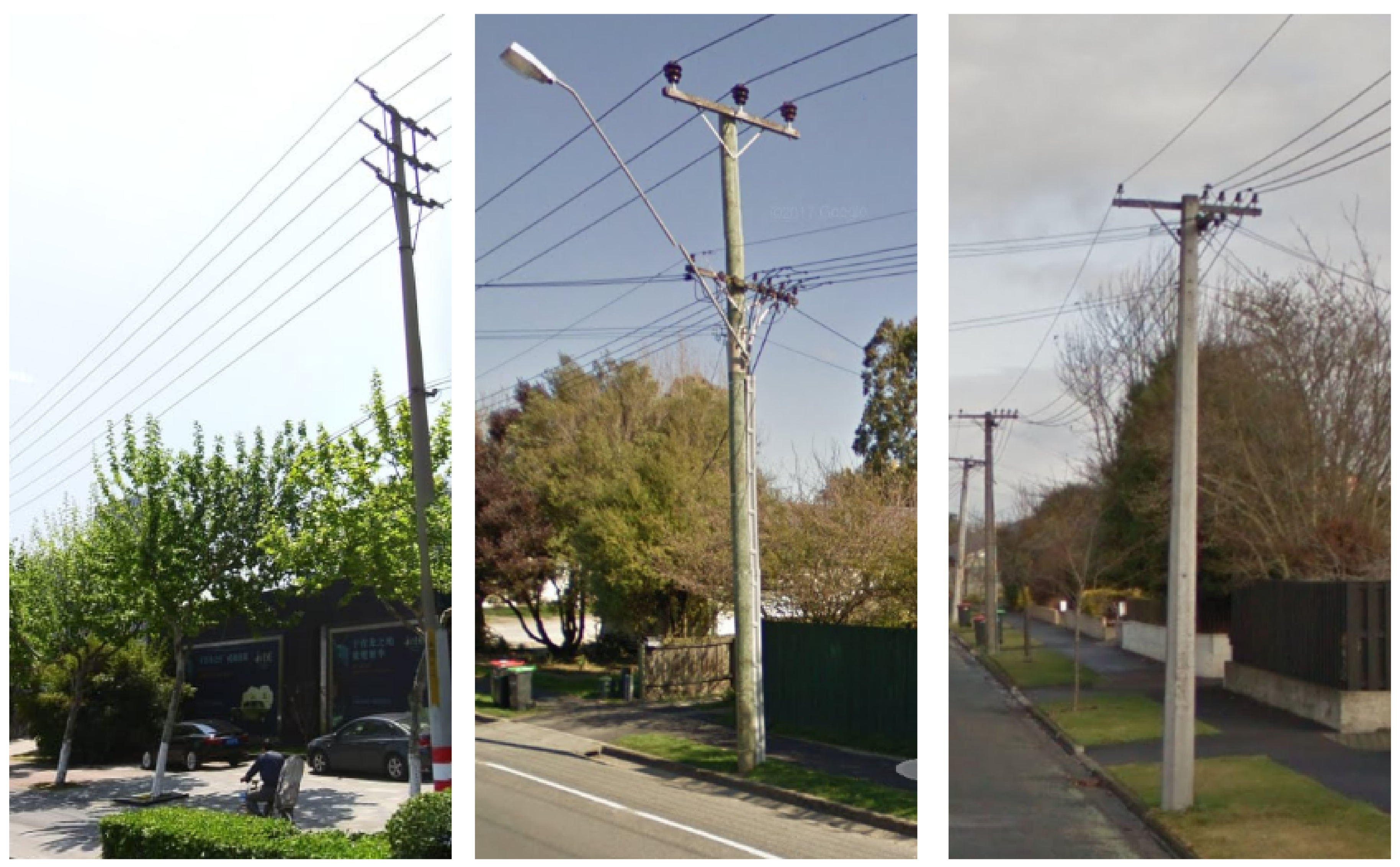
The method presented in this paper is compared with the work by Cheng et. al, as it is the closest previous attempt at realising the goal of automated low cost vehicle surveys of electrical infrastructure. However the equipment employed by Cheng requires significantly more investment, consisting of multiple LiDARs, IMUs, and a high accuracy GPS, compared to the single VLP-16 used here. The conductor spans in Cheng’s work are all similar, consisting of 6 conductors stacked vertically in two groups of three; see Figure 8. In contrast the spans used in this work are from a well established portion of the network where the infrastructure is less homogeneous. Unfortunately Cheng’s dataset was unavailable for direct comparison, however the same metrics are provided to allow for meaningful comparisons to be made in the following sections.

5. Results

5.1. Sag Estimation

The sag estimation performed well on the Hounslow dataset, fitting valid sag models to all primary and secondary conductors; see

Table 1. Sag model recovery performance on the Hounslow dataset.

	Correct	Error
Primary	6	0
Secondary	3	0
Crossing	1	3

. Only one of the four spans crossing the road was recovered. The recovered span took a longer diagonal path across the road, while the other three spans were too short to generate enough valid COMs.

The sag estimation also performed well on the Gilberthorpes dataset, fitting sag models to all 18 primary spans and 7 of 8 secondary spans; see

Table 2. Sag model recovery performance on the Gilberthorpes dataset.

	Correct	Error
Primary	18	0
Secondary	7	1
Crossing	10	9

. Over half of the spans crossing the road were also fitted, this better performance is primarily due to the road crossing spans being longer than those in the Hounslow dataset.

5.2. Sag Model Rejection

On both the Hounslow (

Table 3. Sag model rejection performance on the Hounslow dataset.

	Accepted	Rejected
Valid Sag Model	11	0
Invalid Sag Model	0	5

) and Gilberthorpes (

Table 4. Sag model rejection performance on the extended Gilberthorpes dataset.

	Accepted	Rejected
Valid Sag Model	54	0
Invalid Sag Model	10	8

) datasets there were no falsely rejected sag models. On the Hounslow dataset, all incorrect sag models were rejected and 45% were rejected on the Gilberthorpes dataset.

5.3. 1-Dimensional Mean Shift Clustering

The 1-Dimensional Means Shift clustering was performed using only the cross span-wise component of the conductor points on the clustering plane. This method was able to cluster all primary conductors with a kernel size of 3 and 4 cm on the Hounslow dataset; see

Table 5. This table shows the number of successfully clustered conductors using 1D Mean Shift Clustering with various bandwidths. All conductor spans from the Hounslow dataset were tested.

Bandwidth	Primary	Secondary
3 cm	24	7
4 cm	24	7
5 cm	23	7
6 cm	14	7
7 cm	6	7
8 cm	0	7

. With larger kernels, the primary conductors began being clustered together due to their proximity. All secondary conductors were correctly clustered regardless of the kernel size because they all had larger clearances.

For the primary spans in the Gilberthorpes dataset, all top-level conductors were clustered except for when using a 3cm kernel; see

Table 6. This table shows the number of successfully clustered conductors using 1D Mean Shift Clustering with various bandwidths. Conductor spans with two layers from the extended Gilberthorpes dataset were tested.

Bandwidth	Primary	Secondary
3 cm	53	84
4 cm	54	78
5 cm	54	71
6 cm	54	58
7 cm	54	46
8 cm	54	42

. With the smaller kernel the failure was caused by splitting a single conductor into many clusters resulting in its rejection due to not being distributed along the entire span.

5.4. 2-Dimensional Mean Shift Clustering

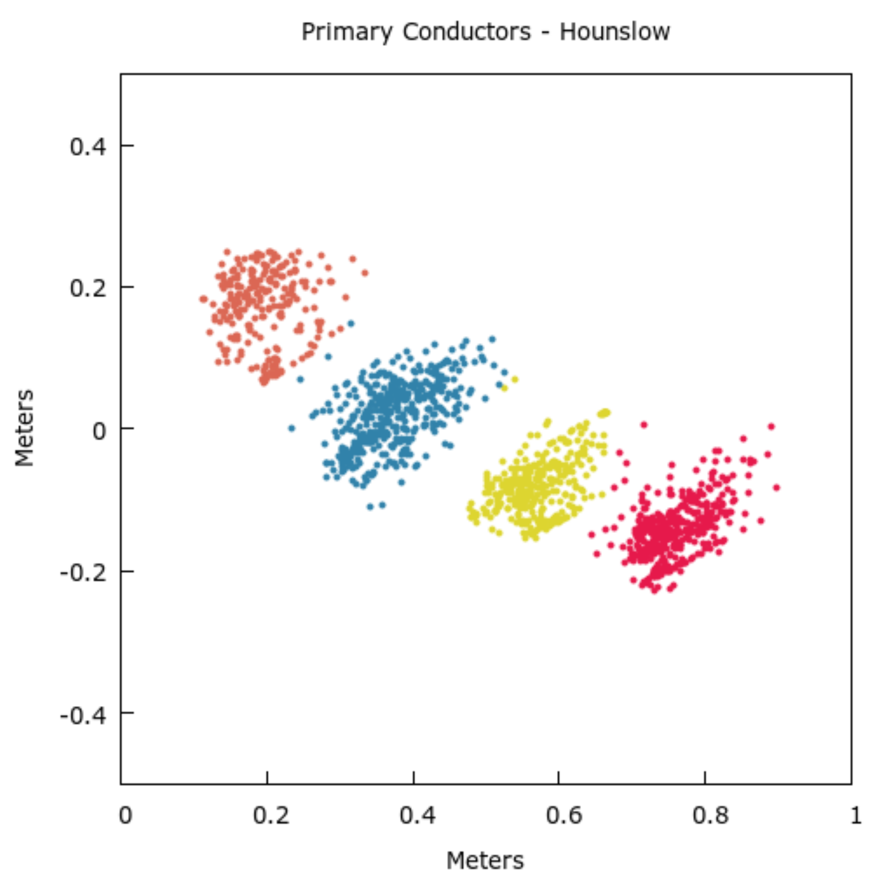
The 2-Dimensional Mean Shift Clustering used both the cross span-wise and vertical components of the points on the clustering plane. This approach performed better over a broader range of kernel sizes than its 1-Dimensional counterpart for the Hounslow dataset; see

Table 7. This table shows the number of successfully clustered conductors using 2-Dimensional Mean Shift Clustering with various bandwidths. All conductor spans from the Hounslow dataset were tested.

Bandwidth	Primary	Secondary
3 cm	24	4
4 cm	24	4
5 cm	24	4
6 cm	24	4
7 cm	16	6
8 cm	6	7

. Upon closer inspection it can be seen that while only a single level of conductors is being clustered, there is still some cross span-wise overlap between the conductors which will result in less defined boundaries between clusters when only 1-Dimension is considered; see Figure 9. For smaller kernel sizes, not all of the secondary conductors could be clustered.

On the Gilberthorpes dataset the 2-Dimensional Mean Shift clustering was able to recover all top layer conductors for kernel sizes greater than 4 cm. With a kernel size of 4 cm, 82 of the 90 bottom layer conductors were also successfully clustered. A steady drop off in performance in bottom layer clustering was observed for larger kernel sizes due to the merging of close conductors; see

Table 8. This table shows the number of successfully clustered conductors from the extended Gilberthorpes dataset using 2-Dimensional Mean Shift Clustering with various bandwidths.

Bandwidth	Top Layer	Bottom Layer
3 cm	50	78
4 cm	52	82
5 cm	54	74
6 cm	54	63
7 cm	54	50
8 cm	54	43

.

5.5. Conductor Recovery Performance

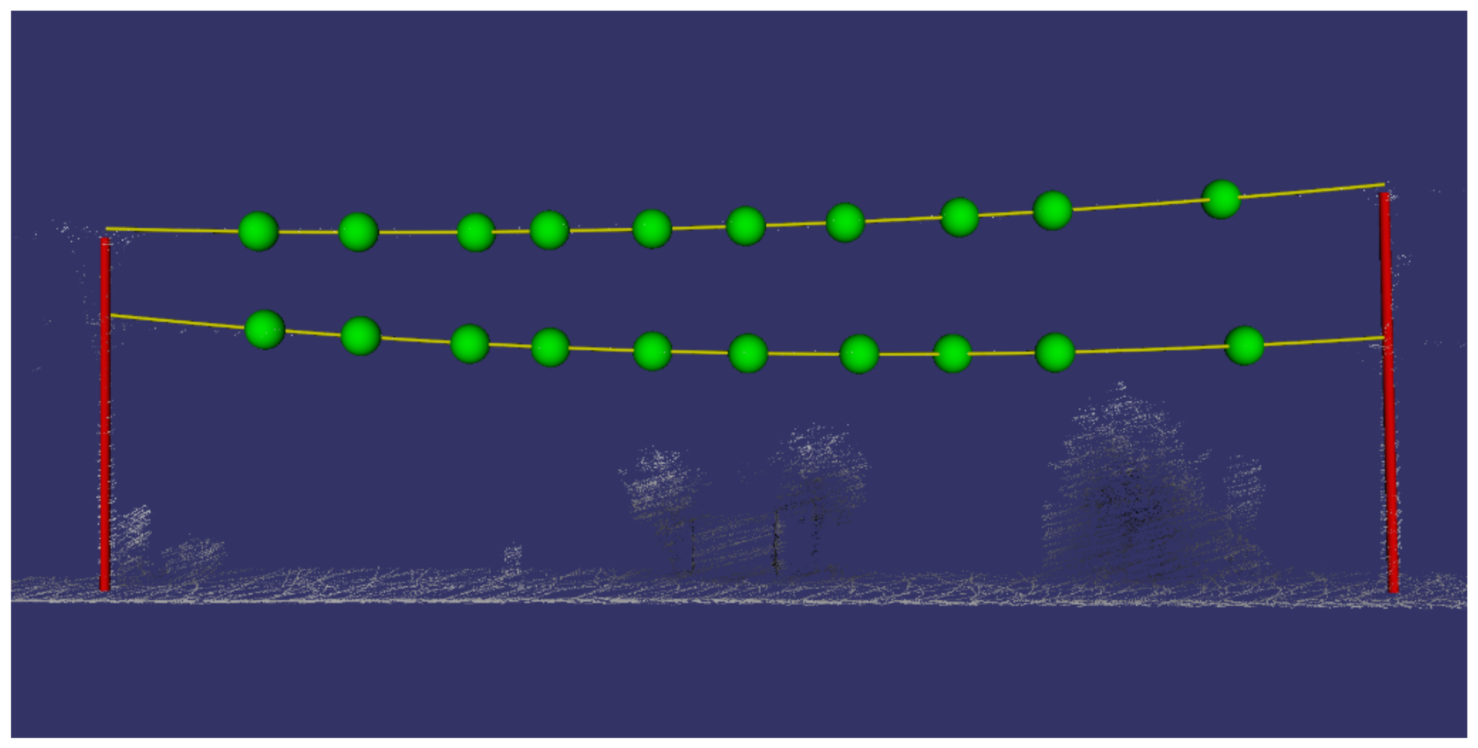
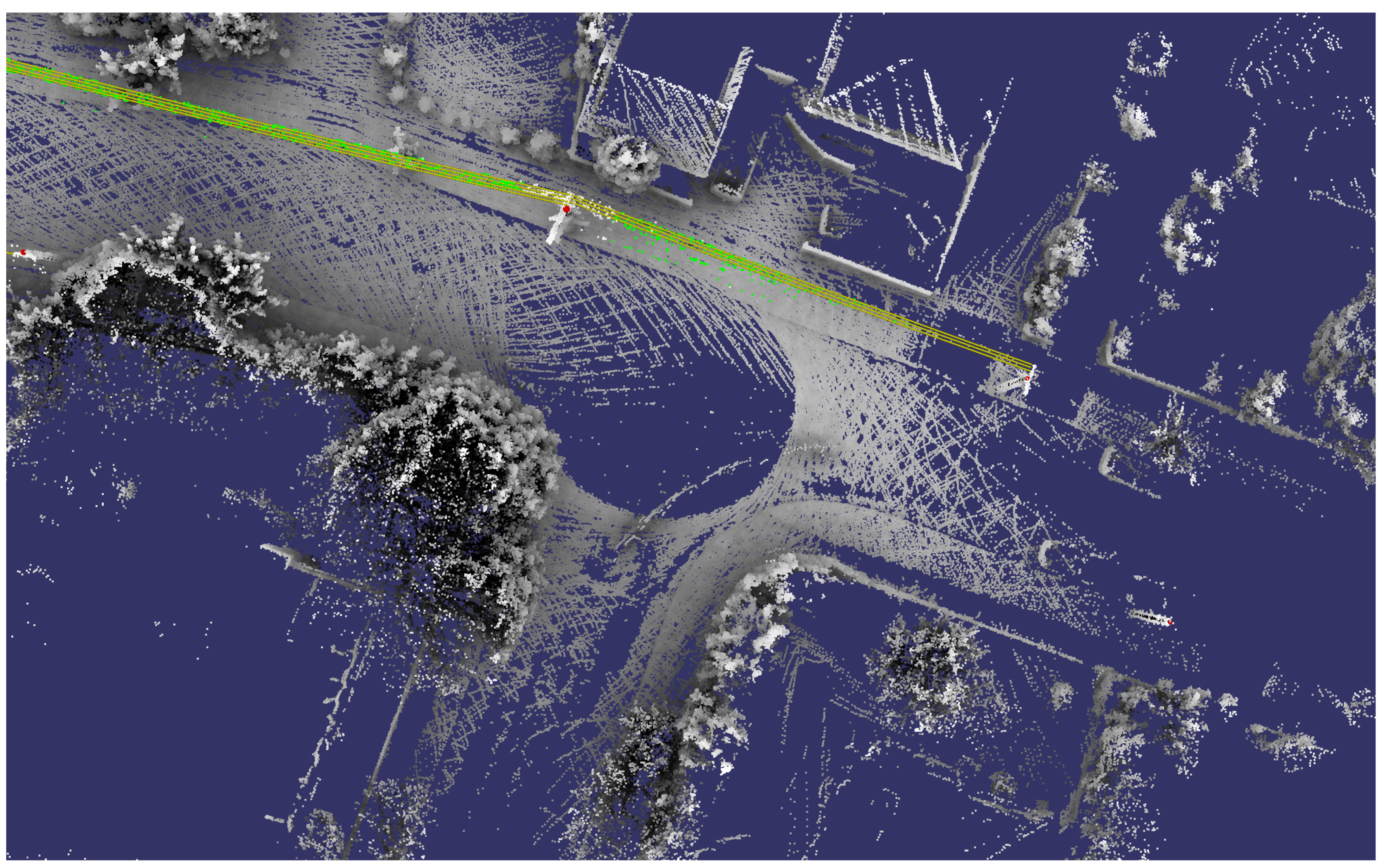
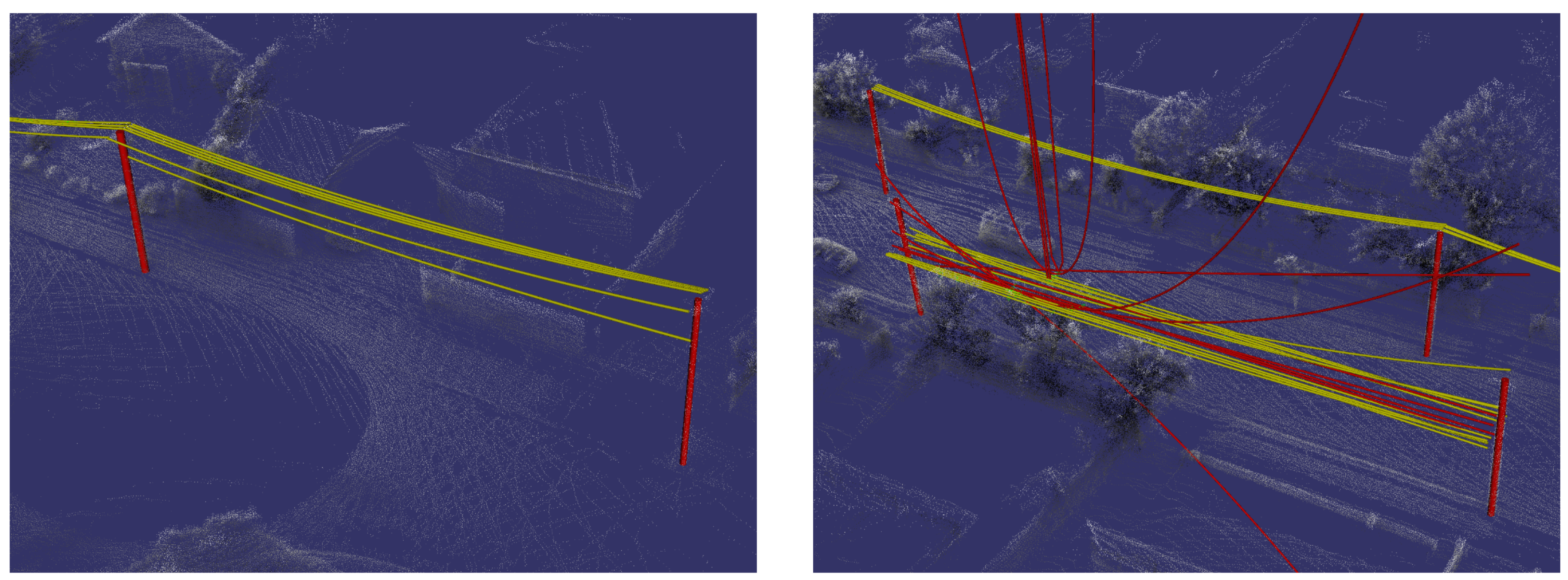
On the Hounslow dataset 23 of the 24 primary conductors, 2 of 3 secondary, and 1 of 4 crossing conductors were recovered; see

Table 9. Final output on Hounslow dataset using 2-Dimensional Mean Shift Clustering with a bandwidth of 4 cm.

	Conductor	Non-Conductor
Modelled Conductors	26	0
Missed Conductors	5

. There were no false positive conductors recovered. The one primary conductor that was missed belonged to a span that was not well observed at the end of the scan; see Figure 10. The conductor was clustered but then rejected by the rule requiring that conductors have points distributed along the entire span. If this rule is removed, the conductor can be recovered (Figure 11) at the cost of losing robustness to non-conductor objects on the clustering plane.

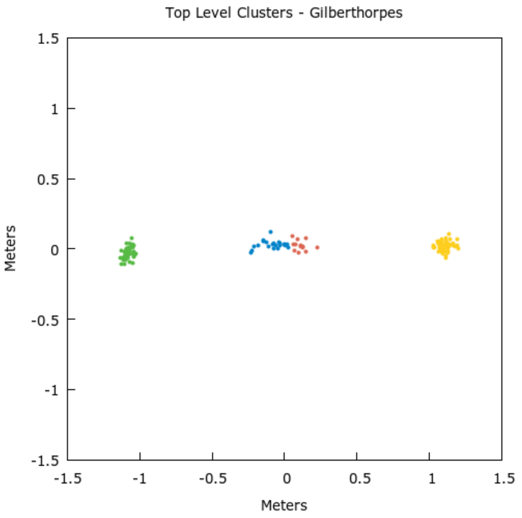
On the Gilberthorpes dataset 90% of the top level conductors and 91% of the bottom level conductors were recovered from the primary spans; see

Table 10. Final output on extended Gilberthorpes dataset using 2-Dimensional Mean Shift Clustering with a bandwidth of 4 cm.

	Top	Bottom	Crossing	Secondary
Modelled Conductors	49	74	5	6
Missed Conductors	5	7	14	2

. 25% of the conductors crossing the road and 75% of the secondary conductors were recovered. All of the missed top level conductors were the centre conductor. These centre conductors weaved between the left and right of the poles which caused the projected points to be spread horizontally on the clustering plane; see Figure 12. This horizontal spread results in the conductor being broken into multiple clusters. Furthermore, the left most points of these clusters will be close to one pole while the right are closer to the other. Because these clusters are more distributed towards a particular end of the span, they tend to be rejected by the rule stating that clusters must be found along the entire length. It is for this reason that these top-level conductors were missed.

On the Gilberthorpes dataset, there were also three falsely recovered conductors. Two of these falsely recovered conductors were the result of two shorter conductor spans being co-linear. While both of the short spans were successfully recovered, they also produced a false positive when treated as a single larger span.

Correctness and Completeness

For comparison with Cheng et al’s work on extraction of power lines in urban environments, we have adopted their two primary metrics.

$$Completeness=\frac{TP}{TP+FN}$$

$$Correctness=\frac{TP}{TP+FP}$$

An important note of difference is Cheng used the length of the conductors, while here the absolute count of conductors has been used. This is due to the difference in the final representation of the conductors. Cheng’s method performs a piecewise recovery of the conductors; thus it is possible to only partially recover a conductor. Our method produces a model constrained in length by the two poles it is attached to, thus it is not possible to partially recovery a conductor; only complete conductor models are produced.

Table 11. Completeness and Correctness for primary conductors in Hounslow and Gilberthorpes datasets.

	Completeness	Correctness
Hounslow - Primary	95.6 %	100%
Gilberthorpes - Top	90.7%	98.0%
Gilberthorpes - Bottom	91.4%	100%
Combined	91.8%	98.6%

shows a break down of the completeness and correctness for our proposed conductor recovery method.

6. Discussions

6.1. Comparison with Existing Work

When compared with the state of the art in urban power line surveying using vehicle-mounted LiDAR, we achieve a similar level of performance. In Cheng’s work, a correctness of 99.1% and completeness of 93.9% was achieved. These numbers show comparable performance with our proposed method; 98.6% and 91.8% respectively. These metrics, however, fail to account for other differences between the systems. While the distances between conductors are not given in Cheng’s works, imagery from the surveyed street indicates that the conductors had significantly more clearance between them than those used in this work; see Figure 8. Many previous methods of conductor recovery, including that presented by Cheng, rely on finding the eigenvectors to traverse along the spans. As previously stated, using eigenvectors is problematic when the conductors are close together. This is because it is difficult to include enough points to generate stable eigenvectors, while not increasing the size of the search space to where it is polluted with points from adjacent conductors. By using a clustering plane instead of conductor traversal, conductors closer together can be recovered with comparable levels of performance.

6.2. Parallel Assumption

One assumption made by the use of a clustering plane is that conductors run parallel to the overall span. While this mostly holds, the centre conductor on the top level of the Gilberthorpes dataset is attached to the cross arm on alternating sides of the pole. This zig-zag path results in a distorted projection of the conductors’ points onto the clustering plane. With larger clustering kernels these distorted clusters could still be recovered, but at the cost of merging the lower level conductors that were closer together. One solution would be to use different kernel sizes for different conductor levels, but this would require prior knowledge of the conductor configurations. Instead, a method similar to sag compensation could be applied to each level of conductors in an attempt to measure how far off parallel the conductors are, and then subtract this difference as is done with sag.

6.3. Failure Modes

On the Hounslow dataset, one primary conductor was missed at the end of the scan where the point-cloud was less uniform and dense. The span where the conductor was missed was only well represented at one end. While the conductor was clustered, it was rejected because it didn’t have points along the entire span. By disabling this rejection rule the missing primary conductor and the secondary telecommunication cable below were recovered. However, by removing this rule, other areas of the scan where trees were inside the conductor search space resulted in erroneous conductors being recovered; see Figure 11. In all fairness, this span should not have been used in the evaluation of this method as the vehicle did not travel the entire length, but its inclusion does better highlight the relation of this rejection rule to the method’s overall performance.

The final failure of note was caused by two aligned short spans. While the conductors belonging to the two spans were correctly recovered, there were two additional falsely recovered conductors produced by combining the two spans into one. The proposed method performs no checks to ensure that the geometry of the poles is valid other than measuring their distance. A possible extension would be to check a candidate span against those around it for conflicting infrastructure.

7. Conclusions

In this article, we have presented a conductor reconstruction method that operates on point clouds collected from vehicle-mounted LiDAR. By using the utility poles to locate the conductor search space, finding the number of conductor levels, and estimating the conductor sag before attempting to cluster and reconstruct the conductors, this method can operate in more challenging environments which previous methods have avoided or only achieved poor performance in. We have shown this method is robust to foliage within close proximity to the conductors and can cluster neighbouring conductors with significantly different point densities.

This method has made an assumption that the conductors run parallel to the conductor search space. While this assumption largely holds true, our proposed method is sensitive to conductor configurations where conductors deviate from parallel. In the future, we plan to implement a method of detecting and compensating for non-parallel conductors using a similar approach as used for managing the conductor sag.

While this method does have some limitations, we believe that it offers a solid foundation for future development and extension. It has an immediate utility to the application of Dynamic Line Rating and could have additional potential use monitoring tree encroachment due to its robustness to nearby foliage.

References

1. Transpower. Clearances and Conductor Spacings; Transpower: Wellington, New Zealand, 2009. [Google Scholar]
2. NZ Standards. ASNZS 7000:2016—Overhead Line Design; Standards Australia Limited/Standards New Zealand: Sydney, Australia; Wellington, New Zealand, 2016. [Google Scholar]
3. Golinelli, E.; Perini, U.; Ogliari, G. A new IR laser scanning system for power lines sag measurements. In Proceedings of the 8th Italian National Conference on Photonic Technologies (Fotonica 2016), Rome, Italy, 6–8 June 2016. [Google Scholar] [CrossRef]
4. HD Electric Company. Cable Distance Meter. 2004. Available online: https://www.transcat.com/media/pdf/CDM-75.pdf (accessed on 1 November 2020).
5. Müller, M.; Hoffmann, J.; Kersting, A. Transmission Line Up-Rating Design Using Survey Data from Airborne Lidar; Cigré: Paris, France, 2006. [Google Scholar]
6. Clode, S.; Rottensteiner, F. Classification of Trees and Powerlines from Medium Resolution Airborne Laserscanner Data in Urban Environments; APRS Workshop on Digital Image Computing: Brisbane, Australia, 2005. [Google Scholar]
7. Jwa, Y.; Sohn, G. A Piecewise Catenary Curve Model Growing for 3D Power Line Reconstruction. Photogramm. Eng. Remote Sens. 2012, 78, 1227–1240. [Google Scholar] [CrossRef]
8. Zhu, L.; Hyyppä, J. Fully-Automated Power Line Extraction from Airborne Laser Scanning Point Clouds in Forest Areas. Remote Sens. 2014, 6, 11267–11282. [Google Scholar] [CrossRef] [Green Version]
9. Sohn, G.; Jwa, Y.; Kim, H.B. Automatic Powerline Scene Classification and Reconstruction Using Airborne Lidar Data. ISPRS Ann. Photogramm. Remote Sens. Spat. Inf. Sci. 2012, I-3, 167–172. [Google Scholar] [CrossRef] [Green Version]
10. Otcenasova, A.; Hoger, M.; Altus, J. Possible use of airborne LiDAR for monitoring of power lines in Slovak Republic. In Proceedings of the 2014 15th International Scientific Conference on Electric Power Engineering (EPE), Brno, Czech Republic, 12–14 May 2014. [Google Scholar] [CrossRef]
11. Mclaughlin, R. Extracting Transmission Lines From Airborne LIDAR Data. IEEE Geosci. Remote Sens. Lett. 2006, 3, 222–226. [Google Scholar] [CrossRef]
12. Jwa, Y.; Sohn, G.; Kim, H.B. Automatic 3D Powerline Reconstruction Using Airborne Lidar Data. In Laser Scanning; Bretar, F., Pierrot-Deseilligny., M., Vosselman, G., Eds.; IAPRS: Paris, France, 2009; Volume XXXVIII. [Google Scholar]
13. Guo, B.; Li, Q.; Huang, X.; Wang, C. An Improved Method for Power-Line Reconstruction from Point Cloud Data. Remote Sens. 2016, 8, 36. [Google Scholar] [CrossRef] [Green Version]
14. Cheng, L.; Tong, L.; Wang, Y.; Li, M. Extraction of Urban Power Lines from Vehicle-Borne LiDAR Data. Remote Sens. 2014, 6, 3302–3320. [Google Scholar] [CrossRef] [Green Version]
15. Liang, J.; Zhang, J.; Deng, K.; Liu, Z.; Shi, Q. A New Power-Line Extraction Method Based on Airborne LiDAR Point Cloud Data. In Proceedings of the 2011 International Symposium on Image and Data Fusion, Tengchong, China, 9–11 August 2011. [Google Scholar] [CrossRef]
16. Wang, Y.; Chen, Q.; Liu, L.; Zheng, D.; Li, C.; Li, K. Supervised classification of power lines from airborne LiDAR data in urban areas. Remote Sens. 2017, 9, 771. [Google Scholar] [CrossRef] [Green Version]
17. Melzer, T.; Briese, C. Extraction and Modeling of Power Lines from ALS Point Clouds. In Proceedings of the 28th Workshop of the Austrian Association for Pattern Recognition, Hagenberg, Austria, 17–18 June 2004. [Google Scholar]
18. McCulloch, J.; Green, R. Density based Recovery of Urban Power Lines using Vehicle-Mounted LiDAR. In Proceedings of the 2018 International Conference on Image and Vision Computing New Zealand (IVCNZ), Auckland, New Zealand, 19–21 November 2018. [Google Scholar] [CrossRef]
19. McCulloch, J.; Green, R. Extraction of utility poles in LIDAR scans using cross-sectional slices. In Proceedings of the 2016 International Conference on Image and Vision Computing New Zealand (IVCNZ), Palmerston North, New Zealand, 21–22 November 2016. [Google Scholar] [CrossRef]
20. McCulloch, J.; Green, R. Utility pole extraction using vehicle-mounted LIDAR for dynamic line rating. In Proceedings of the 2017 International Conference on Image and Vision Computing New Zealand (IVCNZ), Christchurch, New Zealand, 4–6 December 2017. [Google Scholar] [CrossRef]
21. Agarwal, S.; Mierle, K. Ceres Solver. 2010. Available online: http://ceres-solver.org (accessed on 1 November 2020).
22. Velodyne. Velodyne VLP-16. 2017. Available online: https://velodynelidar.com/wp-content/uploads/2019/12/63-9229_Rev-K_Puck-_Datasheet_Web.pdf (accessed on 1 November 2020).
23. Zhang, J.; Singh, S. LOAM: Lidar Odometry and Mapping in Real-time. In Robotics: Science and Systems X; Robotics: Science and Systems Foundation: Berkeley, CA, USA, 2014. [Google Scholar] [CrossRef]
Figure 1. Each window is traversed downwards and new panes are fitted until all points within the window are also included within a pane.
Remotesensing 12 03718 g001
Figure 2. An example of the multiple centre of masses found for each window. Note the bush in the lower right is partially within the conductor search region and thus has centre of masses associated with it.
Remotesensing 12 03718 g002
Figure 3. An example of filtered centre of masses. COMs along the ground are filtered due to their low height, those belonging to the tree are filtered due to their close proximity to each other. The left most COMs on the conductors are filtered because they belong to a window with the incorrect number of COMs.
Remotesensing 12 03718 g003
Figure 4. The remaining centre of masses after filtering. Note all the centre of masses belonging to the ground and the majority of the bush have been removed. The single bush centre of mass remaining fell in a separate window to the rest of the object.
Remotesensing 12 03718 g004
Figure 5. Example of two fitted sag models and the centre of masses used for fitting. Note the centre of mass that was part of a bush in the lower right along with the two directly above in the same window are no longer present when compared with Figure 4.
Remotesensing 12 03718 g005
Figure 6. Using the individual sag models, each level can be individually de-sagged and projected onto the clustering plane. This figure shows the de-sagging process for the upper conductor level; lower levels are each individually processed too.
Remotesensing 12 03718 g006
Figure 7. These figures show the projection of points onto the clustering plane for the span featured in Figure 4 and Figure 5. (a) shows the points projected without sag removal, the points in the lower right belong to a nearby tree. (b) shows the projected points using a single sag model. Note the spread of the points on the lower level has increased when compared with the original points. (c,d) show the upper and lower levels after sag removal using separate sag estimation models. The probability density function is plotted to better show the point density.
Remotesensing 12 03718 g007
Figure 8. Comparison between Cheng’s Nanjing dataset (left), Gilberthorpes (centre), and Hounslow (right). Note the Nanjing image is from 2014 while the LiDAR survey was conducted in 2011.
Remotesensing 12 03718 g008
Figure 9. Example of 2-Dimensional Mean Shift clustering of primary conductors from the Hounslow dataset. Note there is some cross span-wise overlap which results in less defined boundaries if only the cross span-wise component is used.
Remotesensing 12 03718 g009
Figure 10. Example of a poorly observed span which caused a primary conductor to be rejected because it did not contain points along the entire span. Clustered conductor points are rendered green and fitted models are yellow.
Remotesensing 12 03718 g010
Figure 11. Removing the requirement that a conductor cluster must have points distributed along the entire span can increase conductor recovery in less well-observed regions (left) at the cost of less robust rejection of non-conductor objects on the clustering plane (right).
Remotesensing 12 03718 g011
Figure 12. Example of the weaving centre conductor being split into two clusters due to it not being parallel to the span.
Remotesensing 12 03718 g012