Abstract
Carbon dioxide (CO2) is a significant atmospheric greenhouse gas and its concentrations can be observed by in situ surface stations, aircraft flights and satellite sensors. This paper investigated the ability of the CO2 satellite observations to monitor, analyze and predict the horizontal and vertical distribution of atmospheric CO2 concentration at global scales. CO2 observations retrieved by an Atmospheric Infrared Sounder (AIRS) were inter-compared with the Global Atmosphere Watch Program (GAW) and HIAPER Pole-to-Pole Observations (HIPPOs), with reference to the measurements obtained using high-resolution ground-based Fourier Transform Spectrometers (FTS) in the Total Carbon Column Observing Network (TCCON) from near-surface level to the mid-to-high troposphere. After vertically integrating the AIRS-retrieved values with the column averaging kernels of TCCON measurements, the AIRS observations are spatio-temporally compared with HIPPO-integrated profiles in the mid-to-high troposphere. Five selected GAW stations are used for comparisons with TCCON sites near the surface of the Earth. The results of AIRS, TCCON (5–6 km), GAW and TCCON (1 km) CO2 measurements from 2007 to 2013 are compared, analyzed and discussed at their respective altitudes. The outcomes indicate that the difference of about 3.0 ppmv between AIRS and GAW or other highly accurate in situ surface measurements is mainly due to the different vertical altitudes, rather than the errors in the AIRS. The study reported here also explores the potential of AIRS satellite observations for analyzing the spatial distribution and seasonal variation of CO2 concentration at global scales.
1. Introduction
Carbon dioxide (CO2) is considered as one of the primary greenhouse gases (GHGs) in the Earth’s atmosphere [1]. Once CO2 is added to the atmosphere, it exists for a long time: between 300 and 100 years [2]. The global monthly mean CO2 mixing ratio reached about 414.38 parts per million (ppm) in August 2020 [3], which is its highest record since preindustrial times. Understanding and managing the global carbon cycle requires analysis of the spatial distribution and temporal changes of highly accurate CO2 observations.
CO2 concentrations are often measured by in situ surface stations, aircraft flights or satellite instruments. The horizontally sparse surface stations can continuously observe the near-surface CO2 concentration at fixed sites with high accuracy. The vertical profiles of CO2 concentration are measured when the aircraft ascends or descends. However, due to the uneven distribution of ground-based stations, it is not possible to provide the macroscopic monitoring information of CO2 concentrations, especially for the monitoring of CO2 over the ocean, polar region, desert, and other underpopulated areas. Aircraft observations also have similar problems and cannot provide sufficient, stable and continuous monitoring information of atmospheric CO2 concentrations. The advent of satellite observations of CO2 offers exciting opportunities to address some of the above issues.
In the past decade, considerable efforts have been made to extract information about atmospheric CO2 from satellite observations [4]. The TV Infrared Observation Satellite (TIROS), which carried the TIROS Operational Vertical Sounder (TOVS) to provide vertical profiles for climate studies, was first launched on 1 April 1960 [5]. Agencies such as the European Space Agency (ESA), National Aeronautics and Space Administration (NASA), and Japan Aerospace Exploration Agency (JAXA), have also initiated different satellite missions for retrieving estimates of XCO2, including the Scanning Imaging Absorption Spectrometer for Atmospheric Cartography (SCIAMACHY) instrument on Envisat [6], the Atmospheric Infrared Sounder (AIRS) on NASA’s Aqua spacecraft [7], the Orbiting Carbon Observatory (OCO) mission [8,9,10], and the Greenhouse Gases Observing Satellite (GOSAT) [11]. The TanSat (CarbonSat, Tan means “carbon” in Chinese), the first mini-satellite of China dedicated to CO2 detection and monitoring, was launched into space on 21 December 2016 [12]. It fills the gap in GHG-observing technology in China [13]. More and more CO2-measuring satellites, including the Fen-Yun-3D and Gaofen 5, have also been launched and others are also under planning [14]. Table 1 lists these satellite technologies for measuring CO2 in different ways. Since 2002, these satellites have provided researchers with national or global atmospheric CO2 concentration data.

Table 1.
Specification of satellite instruments for Carbon dioxide (CO2) measurements.
The stable, continuous and large-scale atmospheric CO2 concentrations observed by satellites have played an undeniably significant role in observing and understanding the global carbon cycle [15]. Table 1 shows a comparison of the satellites that provide CO2 retrievals with their height range, spatial/temporal resolution, precision and accuracy information. As can be seen from the specification in Table 1, AIRS retrievals use cloud-cleared thermal infrared radiance spectra with an accuracy better than 2 ppm. Compared with other satellite missions, Envisat is an Earth observation mission of the European Space Agency (ESA), which ended on 8 April 2012, following the unexpected loss of contact with the satellite. The precision and accuracy of the Infrared Atmospheric Sounding Interferometer (IASI), the Thermal and Near Infrared Sensor for Carbon Observation Fourier-Transform Spectrometer (TANSO-FTS) and TanSat are lower than those of the AIRS. The height range, spatial/temporal resolution, precision and accuracy of the Orbiting Carbon Observatory 2 (OCO-2) are indeed better than the AIRS, but because it was launched in 2014, there is no time overlap between OCO-2 and HIAPER Pole-to-Pole Observations (HIPPOs) (7 January 2009 to 15 September 2011). AIRS data are still favorable for long-term monitoring and time-series studies which are used by weather prediction centers around the world to improve their forecasts.
Various studies about the inversion and validation of different XCO2 satellite products have been carried out over the last two decades. The CO2 in the troposphere, derived from the SCIAMACHY [16], IASI [17], TANSO-FTS [18,19] and OCO-2 [20], was validated and significantly improved through comparing with the measurements from the ground-based Fourier transform infrared (FTIR) stations network, Comprehensive Observation Network for Tracegases by Airliner (CONTRAIL) [21] or other highly accurate in situ surface and aircraft measurements [22]. All these studies on satellite validation of atmospheric CO2, however, are still in their early stage, and the validation in almost all of these studies has been only carried out based on in situ surface and aircraft measurements, which are horizontally discrete and cannot be very well compared with satellite observations.
In order to make AIRS observations useful for understanding the sources, sinks and the transport of atmospheric CO2 from the surface into the troposphere around the globe, the differences between the AIRS and other reliable accurate in situ surface and aircraft measurements should be validated, understood and characterized. Table 2 lists a collection of major articles and studies related to the validation of AIRS CO2 retrievals. The table summarizes the studies that compare AIRS CO2 retrievals with other different in situ measurements to validate accuracy. Some studies attempt to validate the AIRS CO2 retrievals by comparing them to highly accurate in situ aircraft data and in situ surface measurements.
Table 2.
Summary of the studies using different in situ measurements to compare and validate Atmospheric Infrared Sounder (AIRS) CO2 retrievals.
The mixing ratio of carbon dioxide in the troposphere was derived from the AIRS observations with a high spectral resolution and compared to the aircraft measurements [23]. The CONTRAIL observations obtained by commercial airliner Japan Airlines (JALs) from April 1993 to March 2003 between Japan and Australia were analyzed and reported by Mastsueda et al. [24], which covered the altitude range of 9–13 km, and provided us with knowledge on CO2 distributions in the mid-to-upper troposphere. The retrieved seasonal cycle of the AIRS and its latitudinal dependence were well aligned with aircraft CO2 in situ measurements made at the same altitude range [25]. The AIRS, compared to the aircraft flask CO2 measurements obtained by Matsueda et al. over the Western Pacific, demonstrated skill in tracking the measured 5-ppmv seasonal variation with an accuracy of 0.43 ± 1.20 ppmv [26]. The validation of AIRS retrievals of CO2 via comparison to in situ measurements indicated that the AIRS allowed the monitoring of the distribution of global CO2 in the free troposphere on a weekly basis [27,28]. A methodology for comparing an offline observation of AIRS CO2 with all accessible aircraft measurements of NOAA Earth System Research Laboratories (ESRL)/ Global Monitoring Division (GMD) during 2005 was also proposed [29]. The HIAPER Pole-to-Pole Observations (HIPPOs) were used to evaluate GOSAT, the Tropospheric Emission Spectrometer (TES) and AIRS remote sensing estimates of CO2 [30]. CO2 concentrations measured by aircrafts are closer in altitude to what the AIRS measured, but the difference (1–2 ppmv) found in previous studies could be simply due to the averaging kernel of the AIRS which integrate CO2 concentrations across a wide swath of the mid-to-upper troposphere; thus, the same air was not sampled.
Mid-tropospheric CO2 data retrieved from the AIRS were validated with five ground-based station measurements, illustrating a good agreement in the Northern Hemisphere which had a monthly average accuracy better than 3 ppmv [31]. The further accuracy comparisons of CO2 data derived from the AIRS, SCIAMACHY and GOSAT with the ground-based data from six sites showed that the CO2 retrieved from the AIRS was in excellent agreement with the ground-based data and the most of correlation coefficients were more than 0.9 [32]. The comparison analysis of the global carbon concentration column derived from the SCIAMACHY, AIRS and GOSAT with surface station measurements indicated that the AIRS could reflect the distribution and changes of CO2 very well [33]. The reliability of the mid-tropospheric CO2 data derived from the AIRS was confirmed by comparing with atmospheric CO2 concentration data from GAW ground-based station observations in Malaysia and the deviation between two datasets was less than 1 ppm [34]. From the above studies, CO2 concentrations at the surface are often 2–3 ppmv deviated from that in the mid-to-upper troposphere directly above the same spot on the surface, due to surface sources and sinks that most directly influence the near-surface air. The surface flask data sampled in the boundary layer cannot be used as the estimates representing the mid-to-upper troposphere. The CO2 mixing ratio varies across the different parts of the column, from the near surface reflecting the surface fluxes most strongly to the mid-troposphere reflecting fluxes at broader time/space scales, and the comparison of different measurements reflect the underlying variability. Since these in situ surface measurements that measure CO2 in different vertical portions of the atmospheric column are much lower than what the AIRS measures, the meaning of this direct comparison is arguable. These direct comparisons to surface in situ data, which have been drawn in most of the current studies, are not very useful for validating the AIRS data.
Rather than being acceptable, this level of difference will seriously skew the estimates of sources and sinks of CO2 at the surface, if used in an atmospheric flux inversion. This will lead to incorrect assumptions about what processes drive these fluxes and models for predicting future CO2 levels, defeating the purpose of looking at the AIRS CO2 data in the first place.
The direct validation of the AIRS observations to in situ measurements was not statistically correct due to lack of spatio-temporal coincidence between different measurements. Besides, the peak sensitivity of AIRS CO2 retrievals provided by NASA is broadly in between 6 and 8 km at mid-latitudes, because they are mid-tropospheric estimates rather than CO2 profiles [35]. Therefore, the in situ surface and aircraft profiles should be vertically integrated with reference to the surface and flying altitudes in order to better validate CO2 concentrations of the AIRS.
Therefore, we believe that a real attempt at validating the AIRS CO2 data would be useful. This might involve comparing individual AIRS retrievals to collocated in situ data which has a high accuracy. Collocated data here include both horizontally and vertically collected data. Hence, we attempt to compare the in situ surface data (GAW), full column XCO2 data from the Total Carbon Column Observing Network (TCCON) and in situ aircraft data (HIIPPO) with mid-to-upper tropospheric CO2 data from the AIRS, on equal terms—that is, sampling the same portion of the vertical column.
The vertical profile information in the TCCON estimations can be integrated with the same weighting as it is embodied in the other CO2 profile data.
This paper presents the results of a study on spatio-temporal validation of AIRS CO2 observations using the GAW, HIPPOs and TCCON. The study aims to explore the potential of AIRS satellite observations for monitoring and analyzing CO2 concentrations at global scales. The specific objective of this paper are (1) to study the potential of the combination of high-resolution in situ surface and aircraft measurements for validating AIRS observations by using GAW observations, HIPPO aircraft measurements, TCCON column data and AIRS-retrieved observations; (2) to develop the method and the parameters for validating AIRS using in situ surface and aircraft measurements by vertically integrating the high-resolution HIPPO in situ aircraft and AIRS profiles with column averaging kernels of FTS measurements; (3) to inter-compare the AIRS observations with GAW, TCCON (1 km, 5–6 km) and HIPPO-integrated profiles for understanding the differences of CO2 at their respective altitudes; (4) to analyze the spatial distribution, rising trend and seasonal variation using monthly averaged AIRS observations. The results of the integration, comparison and analysis are also discussed.
2. Datasets and Methods
2.1. Datasets
To assess the derived sensitivity of the AIRS CO2 observations, we selected GAW observations, HIPPO aircraft observations and TCCON column measurements to validate NASA’s AIRS satellite retrieval data. The following sub-sections briefly describe these datasets.
2.1.1. NASA’s AIRS Satellite Data
NASA’s AIRS satellite datasets were used and validated against the GAW, HIPPOs and TCCON in this paper. The NASA Aqua spacecraft carries AIRS instrument, which is an A-Train satellite following 705 km orbits and was launched on 4 May 2002 [36].
AIRS data products contain data at four levels: Level 0, Level 1, Level 2 and Level 3 [39]. The AIRS data are assumed as the initial state for the Vanishing Partial Derivatives (VPDs) retrieval algorithm that separately determines the tropospheric CO2 mixing ratio. The AIRS satellite data used in this paper are AIRSX3C2M (AIRS/Aqua L3 Monthly CO2 in the free troposphere (AIRS + AMSU) 2.5° × 2° V005) from 1 September 2002 to 29 February 2012, which has more overlapped time with the HIPPOs to compare and validate. NASA has also provided another dataset named AIRS3C2M (AIRS/Aqua L3 Monthly CO2 in the free troposphere (AIRS only) 2.5° × 2° V005) from 1 January 2010 to 28 February 2017, which can be used in the future work. They are available from the NASA Goddard Earth Sciences (GES) Data and Information Services Center (DISC) (http://disc.sci.gsfc.nasa.gov/).
The AIRS, a high-resolution infrared spectrometer, covers a wide wavelength range from 3.7 to 15.4 µm, with 2378 spectral channels [37]. As a portion of the NASA’s Earth Observation Satellites (EOSs), the AIRS is considered as one of the most reliable products of CO2 observation data at a global scale [38]. The data have become important tools for improving numerical predictions and supporting climate studies.
2.1.2. HIPPO Airplane Information
The HIPPO research project, funded by the US National Science Foundation (NSF), aims at investigating GHGs, aerosols particles, reactive species and CO2 isotopes. The program is overseen by the Earth Observing Laboratory (EOL) of the National Center for Atmospheric Research (NCAR) [40].
The objectives of HIPPOs are to address the issue of detecting surface GHG emissions, fluxes and transports. Its in-depth information can be utilized to validate both satellite observations and global climate models. The HIPPOs include five worldwide aircraft programs that measure the air from 85°N to 67°S across seasons [41]. Most vertical profiles range from elevations of roughly 0.3 to 8.5 km, but may sometimes go over 14 km.
All HIPPO data are available at EOL data archive (http://www.eol.ucar.edu/field_projects/hippo). The HIPPO datasets contain values (e.g., CO2 observations) and auxiliary data (e.g., Coordinated Universal Time (UTC) and altitude).
Currently, there are five HIPPO flight paths during five different periods. Three instruments have been used to measure CO2, including the Harvard Quantum Cascade Laser Spectrometer (QCLS), the NCAR Airborne Oxygen Instrument (AO2) and the Observation Middle Stratosphere (OMS) CO2 instrument onboard the HIPPO aircrafts (http://data.eol.ucar.edu/master_list/?project=HIPPO-1) [42].
2.1.3. Ground-Based Data
GAW Surface Data
Using eddy covariance towers or wireless sensors networks to obtain atmospheric CO2 concentrations has increasingly become an effective way to monitor the CO2 concentrations on a local scale. In addition to this approach, the commonly adopted measurement method is a ground-based measurement from the Global Atmosphere Watch (GAW) program of the World Meteorological Organization (WMO). The GAW program facilitates the measurements of GHGs in the air environment through a system of stations situated in more than 50 nations [43]. GAW observes the changes and trends in physical and chemical parameters of air composition and evaluates the environmental influences [44]. The GAW observing project provides datasets and services to the decision makers and the public for scientific evaluation and forewarning of changes in the air composition that may have adverse effects on environment [45].
The WMO’s World Data Center for Greenhouse Gases (WDCGGs) controls, archives and distributes the surface station flask data, which provides efficient and dependable meteorological measurements for monitoring the atmospheric environment of the Earth.
TCCON Column Data
The TCCON is a worldwide observing system of ground-based FTSs that records direct solar spectrum in the near infrared. It is associated with the network for the GAW program and the Detection of Atmospheric Composition Change Infrared Working Group (NDACC-IRWG) [46].
The TCCON achieves an accuracy and precision of 0.3 and 0.1 ppm, respectively, in total column measurements and produces a fundamental validation resource for remote sensing observations [47]. It provides accurate measurements of the column average XCO2 at more than a dozen operational sites worldwide. The sites are generally located at low altitudes, where the biosphere/ocean exchange has the most impact on the atmospheric concentrations [48].
The GGG2014 TCCON data used in this study can be obtained from the TCCON Data Archive (http://tccon.ornl.gov/), provided by the Carbon Dioxide Information Analysis Center (CDIAC). The precision of the latest version has been improved through comparing with that of GGG2014 by correcting laser-sampling errors and adding more aircraft and AirCore profiles as bias correction data [49].
TCCON observations are retrieved to provide a long-term, almost continuous time series to assist vertical verification as a transfer standard between in situ measurements and satellite observations, and to help better understand carbon cycle processes [50].
In this paper, the XCO2 data retrieved with AIRS, GAW and HIPPO are validated against the collected ground-based measurements at TCCON sites listed in Table 3.
Table 3.
Geolocation and reference of each TCCON station used in comparison and validation.
2.2. Methods
The spatio-temporal validation method is to inter-compare mid-to-upper tropospheric CO2 data from AIRS retrievals with collocated highly accurate CO2 observations (GAW, TCCON and HIIPPO) based on vertical integration method. The nominal precision and accuracy for these highly accurate CO2 measurements are listed in Table 4.
Table 4.
Precision and accuracy of highly accurate CO2 measurements (Unit 1: ppmv).
At present, there are more than 300 GAW ground-based observation stations for collecting and distributing atmospheric GHG data, and about 212 of these are for monitoring atmospheric CO2 concentrations. GAW observations have decent accuracy, but are restricted to altitude, so additional datasets (HIPPOs and TCCON) are needed for the surface and satellite retrievals. Most of the TCCON sites are close to GAW ground stations, which provide a useful means for validating AIRS satellite retrievals at different elevations with GAW surface observations. The sketch of spatio-temporal validation among the GAW, HIPPOs, TCCON and AIRS are shown in Figure 1.
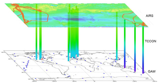
Figure 1.
Sketch of spatio-temporal validation: Global Atmosphere Watch Program (GAW) surface stations (blue dots on the floor), Total Carbon Column Observing Network (TCCON) retrievals (colorful columns), HIAPER Pole-to-Pole Observation (HIPPO) flight paths (orange lines) and AIRS observations (colorful ceiling).
In the sketch of spatio-temporal validation, the blue dots on the floor represent the GAW surface stations, the colored columns represent the TCCON retrievals, the orange lines indicate the HIPPO flight paths, and the colored ceiling represent the AIRS observations. Taking the TCCON column as a bridge, the vertical column of the TCCON is sampled and compared with other CO2 observations from near-surface level to mid-to-high troposphere.
Figure 2 illustrates the overall process of this study which includes three stages: First, the TCCON column averaging kernels and apriori profiles are used to vertically integrate HIPPO aircraft and AIRS retrievals based on kernel-smoothing method. Second, the AIRS-integrated profile is compared with highly accurate HIPPO aircraft profile at flying altitude; third, different portions of the TCCON vertical column from near-surface level to mid-to-high troposphere are sampled to compare with CO2 observations retrieved by AIRS and highly accurate GAW at different altitudes.
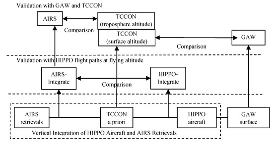
Figure 2.
Overall process of spatio-temporal validation of AIRS CO2 observation.
When inter-comparing measurements made by remote sounders, it is necessary to consider the differing characteristics of the observing system [61]. When inter-comparing AIRS, GAW, HIPPO and TCCON observations, we used the vertical integration method based on averaging kernels and apriori to kernel-smoothing.
After vertical integration of HIPPO aircraft and AIRS retrievals, multiple HIPPO routes can be aggregated into a comprehensive HIPPO-integrated profile and the AIRS-retrieved values could also be regarded as the AIRS-integrated profile from 6 to 8 km. Therefore, the AIRS-integrated profile can be compared with HIPPO profile at the aircraft flying altitude. Then, AIRS, TCCON (5–6 km), GAW and TCCON (1 km) CO2 measurements are compared, analyzed and discussed at their respective altitudes. In this study, the horizontal and vertical comparisons in the spatio-temporal framework were performed at as many as possible different locations and times of year to characterize the AIRS retrieval biases as broadly as possible.
2.2.1. Validation Sites and Dates
TCCON Sites vs. HIPPO Flight Paths
The TCCON can provide very useful means for validating AIRS satellite retrievals at different elevations with HIPPO aircraft high-resolution observations. The accuracy of the TCCON differs at locations, whose single XCO2 measurement (approx. 90 s) is usually less than 0.25 (1-sigma) if it is under a clear sky or partly cloudy conditions (maximally 5% fractional change in solar intensity) and the solar zenith angle is less than 82° [48]. The HIPPO completed campaign consists of numerous flights from December 2008 to September 2011 (see the orange lines in Figure 3). To estimate the accuracy of AIRS XCO2 observations, we use purple dots as shown in Figure 3 to display a dozen operational TCCON sites at different locations and altitudes.
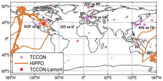
Figure 3.
Overlay of TCCON site locations (purple dots) and HIPPO flight paths (orange lines).
In all TCCON sites, sufficient flight data were collected to conduct comparison analysis based on the average values, except for those sites with no flight. The locations and dates of the HIPPO flights over TCCON sites are given in Table 5. There are three overlapped TCCON sites, including Lamont (OC), Park Falls (PA) and Darwin (DB), which can be used to compare with HIPPO flight profiles. The first HIPPO mission (HIPPO-1) campaign [50] included cross sections of the globe from the North Pole to the South Pole with vertical profiles over the TCCON site Lamont during 2009–2011.
Table 5.
HIPPO flights over TCCON sites. The TCCON site, HIPPO missions, locations, TCCON site height, altitude range of the HIPPO profiles and overlap dates are listed.
GAW Stations vs. TCCON Sites
To estimate the accuracy of global XCO2 observations, we selected the GAW surface stations and TCCON sites at different locations and altitudes as shown in Figure 4. The selected locations of GAW and TCCON sites are appropriate choices for several reasons: (1) the GAW stations should be as close to the TCCON sites as possible; (2) the time interval of the comparisons among the GAW, TCCON and AIRS should be as long as possible. Site selection was also subject to the distribution of stations, which may not be evenly distributed and may not be statistically representative.
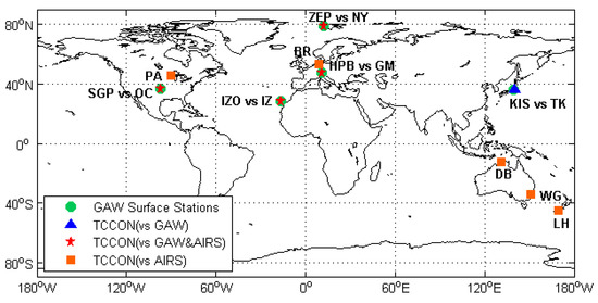
Figure 4.
Locations of GAW surface stations (green dots ●) and TCCON sites (blue triangle ▲, red stars ★ and orange square ■).
The five selected GAW stations were Zeppelinfjellet (ZEP), Hohenpeissenberg (HPB), Kisai (KIS), Izana (IZO), and the Southern Great Plains (SGPs), which were used for comparisons with the five TCCON sites near the surface of the Earth, including Ny Alesund (NY), Garmisch (GM), Tsukuba (TK), Izana (IZ), and Lamont (OC). The TCCON sites located in TK were abandoned because they only had data for 23 months. Instead, Bremen (BR), Darwin (DB), Lauder 120HR (LH), Park Falls (PA), and Wollongong (WG) were taken into account because they had data on a longer period of time for comparison.
2.2.2. Vertical Integration Method
Integration of HIPPO Aircraft and AIRS Retrievals
The AIRS CO2 retrievals provided by NASA are mid-tropospheric estimates, not a CO2 profile, and their extremely high sensitivity is within 6 and 8 km at mid-latitudes [21]. The AIRS-retrieved values integrated vertically with TCCON column data could be regarded as the profile to validate the accuracy of AIRS from 6 to 8 km. Besides, multiple in situ HIPPO aircraft paths also need to be combined and aggregated into a comprehensive vertical HIPPO-integrated profile according to the flying altitude of aircraft.
The TCCON apriori is treated as if it was a wet air mole fraction. When comparing the TCCON data with other data, we found that the difference induced by different H2O formulations is small, but ignoring H2O can cause a significant effect [62]. One site and time-specific TCCON apriori profile per day is included in the GGG2014 netCDF files. These profiles are indexed (note that the index begins at 0) to make it easy to link the apriori profile to a particular measurement. The TCCON is apriori treated as if it is a wet mole fraction. In order to inter-compare the the TCCON data with HIPPO measurements, it must therefore be converted to a dry-air mole fraction by [63]
where the is the dry-air mole fraction of carbon dioxide, is the TCCON apriori profile (vector), and is the mole fraction of H2O [62]. Then the total column-averaged dry-air mole fraction of atmospheric CO2 () can be calculated. TCCON sites are encouraged to obtain in situ profiles as often as possible and to the highest possible altitudes to assure network accuracy and lack of bias. Therefore, the altitude and height range of column at different sites are different. For all sites, the retrieved vertical column abundances of CO2 have been provided in the TCCON archive in the agreed format. Hence, the corresponding XCO2 should be calculated according to the respective height ranges of different sites.
In order to compare TCCON data with high-resolution aircraft and other profile data, we need to use TCCON column averaging kernels and apriori profiles. This information is also covered in the [48] which based on kernels-smoothing method [51]. The main equation is:
where is the smoothed column dry-air mole fraction, is the TCCON apriori column, describes the vertical summation, is the TCCON absorber-weighted column averaging kernel, is the aircraft profile or other model profile, and is the TCCON apriori profile. If = , then it is . There is one apriori profile per local day of measurements, but many TCCON sites measure over two UTC days per local day due to their time zones [62].
In order to properly validate the AIRS CO2 observations, the TCCON column data were integrated vertically with HIPPO in situ aircraft profiles, which is considered as a high-resolution measure of the true atmosphere CO2. The integration equation (Equation (3)) might be utilized as the basis for validating observations and model predictions by the real measurements with detailed vertical resolution and less reliance on the TCCON apriori. For such vertical integration, the scale factor and the mean value of FTS kernels ought to be considered [61].
where denotes the averaging kernel-smoothed profile, is the retrieved profile scale factor, represents the apriori profiles of TCCON, represents the averaging kernels of the FTS measurements which are a formula involving air pressure and solar zenith angle, and is the vertical profile of aircraft CO2 measurements.
For column measurement validation, the profiles need to be vertically integrated according to altitude calculated based on Equation (4), developed according to [53].
where is the averaging kernel-smoothed column from integrating the HIPPO aircraft profile with TCCON apriori profile, and ā is a vector containing the FTS arid compression weight column around kernels. The expression represents the vertical integration weighted with the column mean kernel of the distinction between the HIPPO aircraft profile and the TCCON apriori profile.
Similarly, the mean kernel-smoothed profile and the averaging kernel-smoothed column from integrating the AIRS profile with the TCCON apriori profile are determined by Equations (5) and (6) as follows, developed based on [63].
where is the AIRS CO2-retrieved mid-tropospheric estimation.
Evaluation Parameters
A concentration is the daylight-portion average XCO2 of CO2 observations, which can be one of three possible types: TCCON, HIPPO-integrated or AIRS. The mean absolute error (MAE) is a mean of the proving example of the absolute quantities of the changes. It is used to estimate precision of continuous variables, which can be defined as between two types of observed concentrations of CO2.
where and are the observed CO2 datasets, which can be processed into two token sets as and , and is the number of matched days of XCO2 comparison. The root mean squared error (RMSE) is the square root of the mean of the squares of absolute error, which is a risk function and thus incorporates both the variance of the estimator and its bias.
The average relative error (AVER) is the average of all relative errors, which is defined as the ratio between the absolute error and the magnitude of exact value, which is defined as Equation (9).
3. Results
3.1. Validation with TCCON and HIPPO Flight Paths
The altitude range of flight data varied depending on the air traffic control restrictions. The aircraft equipped with the AO2 and OMS instruments were carried out on 30 January 2009, 20 October 2009, and 9 June 2011 over Lamont (36.6°N, 97.5°W). The largest altitude range of HIPPO flight data was obtained over the TCCON site Lamont (OC), where a lower altitude range (0.4–2.0 km) and higher part of the profile (2.0–13.0 km) were obtained together on 30 January 2009. Based on the above criteria, the TCCON sites located in the Lamont (OC) site (red star in Figure 3) were taken into account because this site had the maximum profile data within the overlap location and time for integration. Here, the 10-s merged CO2 data, obtained from the HIPPO-1 and the TCCON CO2 profile on 30 January 2009, were used. The HIPPO-1, TCCON and integrated CO2 profiles over Lamont are shown in Figure 5.
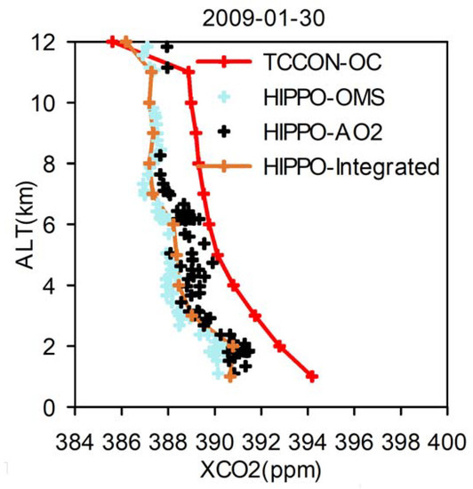
Figure 5.
The integrated CO2 profile by comparing the HIPPO aircraft profiles with the TCCON column data over Lamont (OC) on 30 January 2009. The red line shows the observed TCCON CO2 profile. The light-green and black crosses indicate the observation data of different instruments: HIPPP-OMS and HIPPO-AO2, respectively. The dark-red line shows the integrated CO2 profile.
As shown in Figure 5, the HIPPO aircraft profiles have good accuracy and precision, but lack of smooth continuity in vertical altitude. Thus, additional TCCON column information for the surface and the stratosphere needs to be utilized. There are two instruments—OMS and AO2 in this case—onboard the HIPPO-1 aircraft to measure CO2. A mean (HIPPO-integrated) is applied with HIPPO1-OMS and HIPPO1-AO2.
In this study, a mean (HIPPO-integrated) profile was created from HIPPO1-OMS and HIPPO1-AO2 data. The method for creating a HIPPO-integrated CO2 vertical profile from the HIPPO1-OMS and HIPPO1-AO2 data points is described as follows. First, all of the HIPPO1-OMS data points were averaged within each kilometer to create an altitude-averaged HIPPO-OMS profile. Second, the altitude-average HIPPO1-AO2 was averaged so that its concentration fit to each of the HIPPO1-OMS profiles at each level flight altitude. Finally, the integrated profile of the HIPPOs was created from both the altitude-averaged HIPPO1-OMS profile and HIPPO1-AO2 profile over the Lamont measurement location.
A straight comparison among absolute values therefore makes no sense as the instruments measure CO2 at different altitudes of the atmosphere. In order to obtain the AIRS vertical profiles from 6 to 8 km, the AIRS-retrieved values were integrated vertically with TCCON column data according to Equation (3). The HIPPO and TCCON CO2 data were all collected during the daylight portion of day, and the AIRS Version 5 Level 3 CO2 products from 1 September 2002 to 29 February 2012 contain both the daylight and night portions of day. Therefore, the night-portion AIRS data should be excluded using the tag <DayNightFlag> to better compare profiles, which is embedded in the XML file for each AIRS Level 3 dataset file.
Figure 6 shows the comparison of the AIRS CO2 profile with the TCCON and HIPPO-integrated profile at mid-troposphere over the Lamont site on 30 January 2009. As clearly shown in Figure 6, the AIRS is in good agreement with HIPPO-integrated CO2 data and the TCCON column data have significant bias from the aircraft-based XCO2 of the HIPPOs, especially in the surface. The dependence of biases on altitude can be observed from Figure 6. The minimum deviation of the HIPPOs and TCCON is less than 1 ppm at 12 km, while the maximum deviation is about 4 ppm at 1 km. The average deviation between the HIPPOs and TCCON is 1.92 ppm. The average biases between the AIRS and TCCON is 2.07 ppm. The reason is currently unknown which may be related to the different peak sensitivity altitudes of the AIRS, HIPPOs and TCCON.
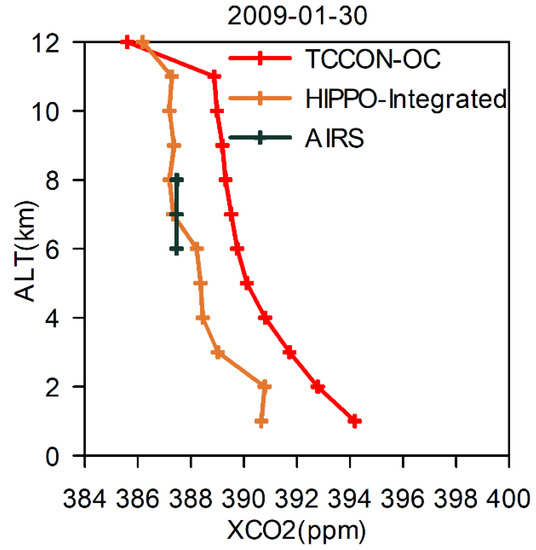
Figure 6.
Spatial validation of AIRS daylit average XCO2 vertical profiles on 30 January 2009. The red line shows the TCCON-OC CO2 profile. The orange line indicates the profile of HIPPO integration. The dark-green line is XCO2 of AIRS at mid-troposphere.
3.2. Validation with GAW and TCCON
The different mean absolute errors, average relative errors and correlation coefficients between TCCON and GAW observations show that the concentrations of CO2 are impacted by a number of factors with various areas and heights, which include but are not limited to surface structure, land cover, vegetation type, and human activities (Table 6).
Table 6.
Results between GAW and TCCON observations. The TCCON and GAW observed data are in mole fraction units: data × 106 = ppm in volume (ppmv).
Table 6 shows the data comparison between TCCON sites and GAW stations near the surface of the Earth. The data listed in this table are the calculations based on monthly average XCO2 in the selected TCCON and GAW stations. The average of is 3.498 ppmv, and the average of is 2.973 ppmv. The value of is less than 2%, and the value of is greater than 0.9030.
The scatter plots (Figure 7) were used to evaluate the retrieved TCCON measurements against the GAW flask surface observations from the same or nearly the same latitude and longitude rages. Figure 7 illustrates the data validation between XCO2 derived from TCCON and GAW surface station observations at five locations (ZEP vs. NY, HPB vs. GM, KIS vs. TK, IZO vs. IZ and SGPs vs. OC) described in Figure 4. The results indicate that a positive correlation exists between TCCON and GAW sites at a global scale, which in turn indicates that the TCCON is an important, reliable observation data source in XCO2 validation research. It can reflect the actual trend of local XCO2 and serve as the basis data for research on the validation of satellite observations of CO2.
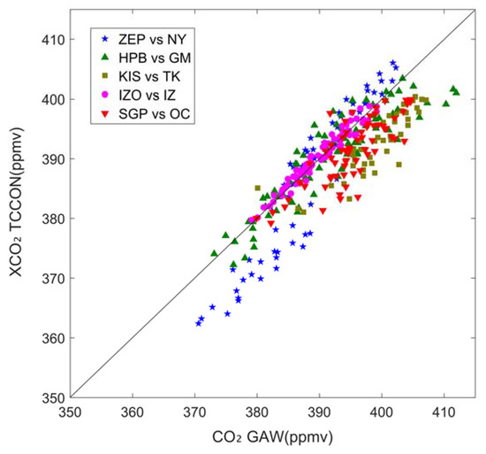
Figure 7.
Validation of TCCON monthly average retrieval results with observational flask CO2 concentration from GAW surface locations: Zeppelinfjellet (ZEP) site vs. Ny Alesund (NY) station (★), Hohenpeissenberg (HPB) site vs. Garmisch (GM) stations (▲), Kisai (KIS) site vs. Tsukuba (TK) station (■), Izana (IZO) site vs. Izana (IZ) station (●), Southern Great Plains (SGPs) site vs. OC station (▼). The black line is the 1:1 line between TCCON retrieval data and GAW data.
Table 7 depicts the comparison between TCCON and AIRS observations at 5–6 km observed altitude. The average of is 2.066 ppmv and the average of is 2.560 ppmv. All of monthly average XCO2 is less than 0.8% and is greater than 0.7.
Table 7.
Validation between TCCON and AIRS observations at 5–6 km observed altitude.
The scatter plots in Figure 8 represent the validation of monthly average XCO2 between TCCON and AIRS observations at AIRS observed altitude and the selected TCCON sites with locations described in Figure 6. The validation result indicates that AIRS observations can reflect the monthly variation of global XCO2 exactly and veritably.
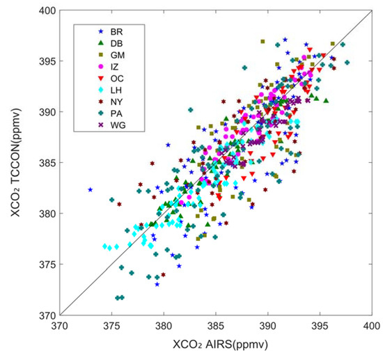
Figure 8.
Validation of monthly average XCO2 between TCCON and AIRS observations at 5–6 km observed altitude: Bremen (BR) (★), Darwin (DB) (▲), GM (■), IZ (●), OC (▼), Lauder 120HR (LH) (♦). NY (🟌), Park Falls (PA) (+) and Wollongong (WG) (×). The black line is the 1:1 line between the TCCON and AIRS.
4. Discussion
4.1. Validation Results Analysis
To evaluate the long-term trends of the total CO2 column concentrations, we inter-compared the mid-to-upper tropospheric CO2 data from AIRS, TCCON and GAW for the period from January 2007 to December 2013, as shown in Figure 9, on equal terms—i.e., sampling the same portion of the vertical column over collocated location. We selected HPB (GAW station) and GM (TCCON site) as comparison sites for analysis because they have good spatial proximity and time continuity. The two sites, HPB and GM, had a contiguously overlapped time span from July 2007 to February 2012.
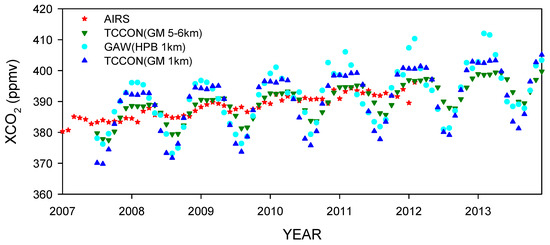
Figure 9.
Comparison of monthly average variation and tendency of CO2 concentrations among the GAW, TCCON (GM 1 km), TCCON (GM 5–6 km) and AIRS.
Figure 9 also shows the time series of the monthly mean CO2 concentrations from different observations. CO2 concentrations measured by the GAW (HPB 1 km) and TCCON (GM 1 km) at the surface are often 2–3 ppmv away from the observations of the TCCON (GM 5–6 km) and AIRS in the mid-to-upper-troposphere above the co-located locations, due to surface sources and sinks that most directly impact the near-surface air. Since the CO2 mixing ratio varies across different parts of the column, from the near-surface (which reflects the surface fluxes most strongly) to the mid-to-upper troposphere (which reflects fluxes at very broad time/space scales), the measurements compared here reflect very different levels of underlying variability.
As shown in Figure 9, GAW located at the HPB site (1 km) and the TCCON located at the GM site (1 km) present higher seasonal amplitudes, which may be caused by vegetation growth, fossil fuel emissions and other human activities. The reasons for this could be attributed to the carbon sources and sinks at the near surface combined with atmospheric mixing determining the spatial distribution and temporal variation of the CO2 in the lower troposphere.
On the other hand, the CO2 concentrations of the AIRS and TCCON (GM 5–6 km) show smaller seasonal amplitudes, which can be attributed to the fact that CO2 is well-mixed within the mid-to-upper troposphere. The results indicate that the amplitude of monthly mean XCO2 fluctuations gradually decreases with increasing altitude and obviously show seasonal characteristics. It appears that atmospheric mixing makes the upper tropospheric CO2 concentrations rather zonal, which indicates that AIRS data inform on very broad features of the surface fluxes only.
Figure 9 further indicates that the monthly variation tendency of XCO2 retrieved from AIRS observations has not only a good consistency with the TCCON measurements from the selected sites at high altitudes, but also good agreement with GAW observations near the surface of the Earth.
The seasonal variation can be further compared to understand the deviation by plotting the amplitude of monthly mean CO2 observations over the year. Figure 10 illustrates the amplitude of monthly mean CO2 observations retrieved from the AIRS (red star), TCCON (GM 5–6 km, green triangle), GAW station (light blue circle, HPB 1 km) and TCCON (GM 1 km, dark-blue triangle) from January to December 2008. In 2008, the annual mean of the AIRS, TCCON (GM 5–6 km) and TCCON (GM 1 km) is 385.4574, 385.7304, and 385.8919 ppmv, respectively, while the annual mean of GAW is 387.1508 ppmv.
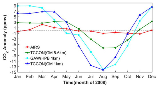
Figure 10.
CO2 amplitude of the AIRS, TCCON (GM 5–6 km), GAW (HPB 1 km) and TCCON (GM 1 km) over 2008.
After subtracting each monthly mean CO2 concentration by annual average, the monthly mean CO2 amplitude is plotted in Figure 10. In 2008, the averaged seasonal cycle amplitude measured at the surface by GAW is about 7 ppmv, whereas in the mid-to-upper troposphere the AIRS observes an averaged amplitude of about 1 ppmv. Additionally, it is worth noting that the maximum values occur approximately three months earlier for the GAW (HPB 1 km) than for the AIRS over the year. The time lag between the AIRS and GAW extremum indicates that the delay was caused by the upward transportation of the seasonal signal from the surface to mid-to-upper troposphere.
Comparing the results (Figure 9 and Figure 10) of this study with previous studies (Table 2), we find that the difference of about 3 ppmv between the AIRS and GAW or other highly accurate in situ surface measurements is mainly due to the different vertical altitude, rather than the errors in AIRSs. Hence, a direct comparison between absolute values from AIRSs and other in situ surface measurements is meaningless as the instruments observe and capture the seasonal variability within different altitude layers of the atmosphere. The validation results demonstrate that AIRS data can provide reliable inter-annual variation information for atmospheric CO2, which are able to provide a great understanding of spatial distribution, temporal variation and vertical exchange of CO2.
4.2. Spatial CO2 Distribution of AIRS
The data file format of AIRS L3 monthly gridded products is Hierarchical Data Format—Earth Observing System (HDF-EOS 2.12) corresponding to HDF 4, the canonical data format for standard datasets retrieved from EOS missions [64]. It contains 4-byte floating derived average values, 4-byte floating standard deviations and a 2-byte integer input counts, as well as the double array (array [0] is latitude and array index [1] is longitude) giving the centers of the 2° (lat) × 2.5° (long) latitude–longitude grids which use the equidistant cylindrical projection.
The nine global views of annual average AIRS XCO2 during 2003–2011 is visualized with MATLAB, as shown in Figure 11. The arithmetic means of the CO2 observations have been averaged into 2° (lat) × 2.5° (long) grids, from 60.0°S to 84.0 ± 4°N latitude and 180.0°W to 180.0°E longitude. The polar regions (between 90°S and 60°S Latitudes) with no retrievals are not considered (white area in Figure 11).
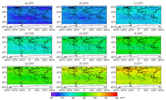
Figure 11.
Global views of AIRS annual average CO2 concentration from 2003 to 2011 as illustrated in (a–i), one for each year’s annual average CO2 concentration. White regions indicate the areas with no retrievals. These figures are based on the compute and visualization of the AIRS level-3 product, which is gridded (2.5° × 2°) data, and they share the same color bar.
The global distribution map of the average of AIRS mean average XCO2 over the 9 years after the high-resolution reconstruction is shown in Figure 12. The areas with the highest value of CO2 concentration in the mid-troposphere are mainly between 30°N and 70°N. From west to east, the ocean areas near Southern Alaska, the central region of the Northern America, Eastern Canada, surrounding areas of Nuuk in Greenland, Central Asia and Northern China, have mean CO2 concentrations of above 385 ppmv in the mid-troposphere during 2003–2011.
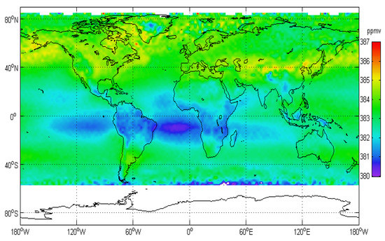
Figure 12.
Global distribution map of the average of AIRS (from 6 to 8 km) annual mean XCO2 during 2003 to 2011 after high-resolution reconstruction. White regions indicate areas with no retrievals.
The areas with low CO2 concentration values are mainly between the Tropic of Cancer and the Tropic of Capricorn. The region in the Atlantic between the equatorial line, latitude 40°W, longitude 20°S, 40°W and the central meridian was the center of the low-value areas. It extends eastward to Eastern Africa and Western India Ocean, and westward to Eastern Pacific Ocean and Western South America.
4.3. Seasonal Variation of AIRS
According to the data retrieved from the AIRS, the mid-tropospheric CO2 concentration was in continuous growth. The average growth rate was approximately 2.1 ppmv/year from January 2003 to December 2011, and the mean of the mid-troposphere CO2 concentration in 2011 exceeded 390 ppmv, while preindustrial atmospheric CO2 concentration levels were around 280 ppmv [65].
During the 9 years from 2003 to 2011, the annual average CO2 concentration in the mid-troposphere at a global scale was in a fluctuating state of growth which increased by 16.8 ppmv. The annual average CO2 concentration in the Northern Hemisphere grew by 17.07 ppmv and in the Southern Hemisphere it increased by 16.47 ppmv from 2003 to 2012. The growth rate of CO2 in the Southern Hemisphere (the areas where effective data were not included) is slightly lower than that in the Northern Hemisphere. The gap between the Northern and Southern Hemisphere is gradually increasing. The annual average CO2 concentration in the Northern Hemispheric troposphere is 1.2 ppmv higher than that in the Southern Hemispheric troposphere.
Figure 13 shows the time–latitude Hovmöller diagrams which were created by averaging the monthly AIRS retrieval results into 2° altitude bins for all longitudes from January 2003 to December 2011. As shown in Figure 13, there is a continuous flow of CO2 from the Northern Hemisphere to the Southern Hemisphere with a time scale. The time cycle in the Northern Hemisphere shows a significant increase around May, followed by a constant decrease, with maximum (peak) in spring (April or May) and minimum (valley) in winter (November or December). The AIRS CO2 concentration in the Southern Hemisphere showed a rising tendency different from those gained in the upper hemisphere. The time cycle of AIRS-retrieved dataset in the Southern Hemisphere shows a small increase followed by a small decrease, with a two-maximum structure in March and November, and a minimum in May.
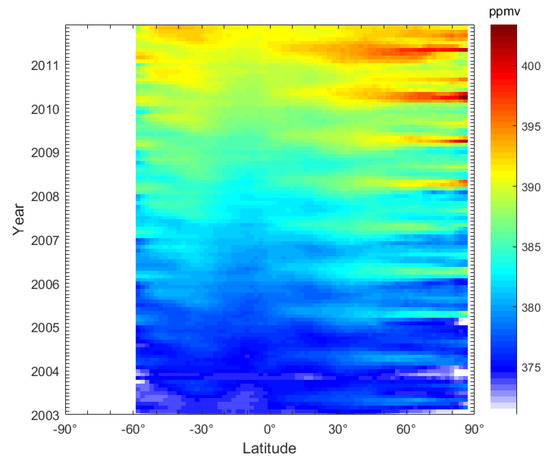
Figure 13.
Time–latitude Hovmöller diagram of monthly average CO2 concentration in mid-troposphere based on AIRS from March 2003 to February 2012. The regions without effective data are not included.
The time series of the monthly average CO2 concentration in the Northern Hemisphere showed a more significant seasonal change circle and the extremum was presented from month to month. The seasonal amplitudes of AIRS-retrieved dataset in the Southern Hemisphere is significantly smaller. This corresponds to what is presently known about the greenhouse effect [66].
Figure 14 illustrates the amplitude of the monthly mean CO2 observations retrieved from AIRS in the Northern (red bar) and Southern (blue bar) Hemisphere. The peak-to-peak fluctuation range of the time variation in the Northern Hemisphere displays the evolution in time as follows: if the rate increases faster, it also decreases faster, and vice versa. A clear amplitude of CO2 variability in the Northern Hemisphere is about 4 ppmv, which is much greater than the amplitude of CO2 time variability in the Southern Hemisphere (1 ppmv).
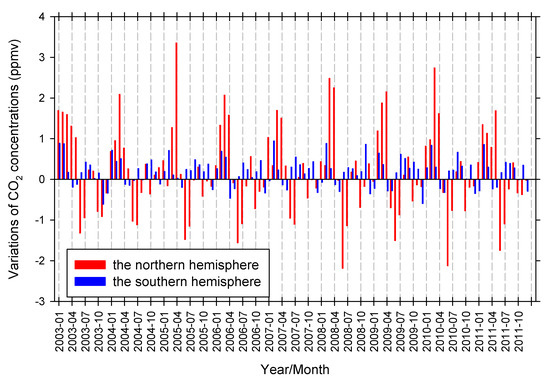
Figure 14.
The amplitude of monthly average CO2 concentration retrieved from the AIRS in the Northern (red) and Southern (blue) Hemisphere.
5. Conclusions
In this paper, a spatio-temporal validation method of AIRS CO2 observations with the XCO2 retrieved from the GAW, HIPPOs and TCCON according to their observation locations and altitudes was proposed for better understanding of the spatial and temporal variation of global XCO2. After the TCCON (wet mole fraction) was apriori converted to a dry-air mole fraction, the high-resolution HIPPO in situ aircraft profiles and AIRS CO2 retrievals were integrated vertically with TCCON column data.
To estimate the accuracy of global XCO2 observations, we selected the GAW surface stations and TCCON sites at different locations and altitudes for two reasons: (1) the GAW stations should be as close to the TCCON sites as possible; (2) the time periods of the comparisons among GAW, TCCON and AIRS should be as long as possible.
Three overlapped TCCON sites, including Lamont (OC), Park Falls (PA) and Darwin (DB), were used for comparisons with HIPPO flight profiles. The largest altitude range and the maximum profile data of HIPPO flight data were obtained over the TCCON site Lamont (OC), where the lower altitude range (0.4–2.0 km) and higher part of the profile (2.0–13.0 km) were obtained together on 30 January 2009, where the scale factor and the averaging kernels of FTS measurements were considered. The method for creating a HIPPO-integrated CO2 vertical profile from the HIPPO1-OMS and HIPPO1-AO2 data points was proposed in this paper to validate the TCCON and AIRS.
The five selected GAW stations were used for comparisons with TCCON sites near the surface of the Earth. With the TCCON sites located in TK adopted because they could be compared with the AIRS for only 23 months, another four TCCON sites which have longer time spans to compare with AIRS observations were added. The monthly variation tendency of XCO2 retrieved from the AIRS shows a decent agreement with the high-altitude TCCON observations from the selected sites, which also presented good consistency with the GAW observations near the surface of the Earth.
The spatial distributions of global AIRS XCO2 showed an obviously higher hemispherical difference with concentrations of 1.2 ppmv in the Northern Hemisphere, in response to the effects by natural sources and human activities. The CO2 concentrations increased yearly, with an average growth rate of approximately 2.1 ppmv/year from January 2003 to December 2011. A significant seasonal variation of CO2 was shown with a peak in April or May and valleys in August or September.
The study results prove the potential of AIRS satellite observations for monitoring and analyzing mid-tropospheric CO2 concentrations at global scales, which will provide new insights into more accurate, sufficient, stable and continuous XCO2 observations. Future work is needed to extend this spatio-temporal validation using an assimilation system. We expect that the CO2 observations that are more reliable will eventually be assimilated into the chemical transport model to calibrate AIRS observations.
Author Contributions
Conceptualization, H.Y., Y.Q. and S.L.; methodology, H.Y., R.X. and Y.X.; software, G.F.; validation, G.F. and Y.X.; formal analysis, H.Y., G.F. and Y.X.; writing—original draft preparation, H.Y.; writing—review and editing, S.L.; funding acquisition, H.Y. All authors have read and agreed to the published version of the manuscript.
Funding
This research was funded by the National Natural Science Foundation of China (grant number 41971335, 51978144 and 51678127) and the project was funded by the Priority Academic Program Development of Jiangsu Higher Education Institutions (PAPD).
Acknowledgments
The authors would like to thank the National Center for Atmospheric Research (NCAR), the Network for the Detection of Atmospheric Composition Change Infrared Working Group (NDACC-IRWG), and the National Aeronautics and Space Administration (NASA), for making their data and code freely available. The TCCON data were obtained from the TCCON Data Archive hosted by CaltechDATA at https://tccondata.org. We thank TCCON PIs for the TCCON measurements at stations of Lamont, Park Falls, Darwin, Ny Alesund, Garmisch, Tsukuba, Izana, Bremen, Lauder 120HR, and Wollongong. The TCCON station at Lamont is supported in part by the OCO and OCO-2 series project. Park Falls TCCON site has received funding from National Aeronautics and Space Administration. Darwin and Wollongong TCCON stations are supported by ARC grants DP160100598, LE0668470, DP140101552, DP110103118 and DP0879468. Local support for Bremen is provided by the European Union (26188, 36677, 284274, 313169 and 640276). Lauder TCCON site has received funding from National Institute of Water and Atmospheric Research and Ministry of Business, Innovation and Employment.
Conflicts of Interest
The authors declare no conflict of interest.
References
- Solomon, S.; Qin, D.; Manning, M.; Marquis, M.; Averyt, K.; Tignor, M.M.B.; Miller, H.L., Jr.; Chen, Z.E. IPCC (Intergovernmental Panel on Climate Change), Climate Change 2007: The Physical Science Basis Contribution of Working Group I to the Fourth Assessment Report of the Intergovernmental Panel on Climate Change; Cambridge University Press: Cambridge, UK; New York, NY, USA, 2007; p. 996. [Google Scholar]
- Available online: https://climate.nasa.gov/news/2915/the-atmosphere-getting-a-handle-on-carbon-dioxide/ (accessed on 8 September 2020).
- NOAA Mauna Loa CO2 Data. Available online: http://co2now.org/Current-CO2/CO2-Now/noaa-mauna-loa-co2-data.html (accessed on 16 October 2020).
- Engelen, R.J.; Serrar, S.; Chevallier, F. Four-dimensional data assimilation of atmospheric CO2 using AIRS observations. Geophysical Research. J. Geophys. Res. Atmos. 2009, 114. [Google Scholar] [CrossRef]
- Chédin, A.; Hollingsworth, A.; Scott, N.A.; Serrar, S.; Crevoisier, C.; Armante, R. Annual and seasonal variations of atmospheric CO2, N2O and CO concentrations retrieved from NOAA/TOVS satellite observations. Geophys. Res. Lett. 2002, 29, 110–114. [Google Scholar] [CrossRef]
- Burrows, J.P.; Hölzle, E.; Goede, A.; Visser, H.; Fricke, W. SCIAMACHY—Scanning imaging absorption spectrometer for atmospheric chartography. Acta Astronaut. 1995, 35, 445–451. [Google Scholar] [CrossRef]
- Engelen, R.J.; Andersson, E.; Chevallier, F.; Hollingsworth, A.; Matricardi, M.; McNally, A.P.; Thepaut, J.; Watts, P.D. Estimating atmospheric CO2 from advanced infrared satellite radiances within an operational 4D-Var data assimilation system: Methodology and first results. J. Geophys. Res. 2004, 109. [Google Scholar] [CrossRef]
- Eldering, A.; O’Dell, C.W.; Wennberg, P.O.; Crisp, D.; Gunson, M.R.; Viatte, C.; Avis, C.; Braverman, A.; Castano, R.; Chang, A.; et al. The Orbiting Carbon Observatory-2: First 18 months of science data products. Atmos. Meas. Tech. 2017, 10, 549–563. [Google Scholar] [CrossRef]
- Eldering, A.; Wennberg, P.O.; Crisp, D.; Schimel, D.; Gunson, M.R.; Chatterjee, A.; Liu, J.; Schwandner, F.M.; Sun, Y.; O’Dell, C.W.; et al. The Orbiting Carbon Observatory-2 early science investigations of regional carbon dioxide fluxes. Science 2017, 358, eaam5745. [Google Scholar] [CrossRef] [PubMed]
- Crisp, D.; Pollock, H.R.; Rosenberg, R.; Chapsky, L.; Lee, R.A.M.; Oyafuso, F.A.; Frankenberg, C.; O’Dell, C.W.; Bruegge, C.J.; Doran, G.B.; et al. The on-orbit performance of the Orbiting Carbon Observatory-2 (OCO-2) instrument and its radiometrically calibrated products. Atmos. Meas. Tech. 2017, 10, 59–81. [Google Scholar] [CrossRef]
- Yokota, T.; Yoshida, Y.; Eguchi, N.; Ota, Y.; Tanaka, T.; Watanabe, H.; Maksyutov, S. Global Concentrations of CO2 and CH4 Retrieved from GOSAT: First Preliminary Results. SOLA 2009, 5, 160–163. [Google Scholar] [CrossRef]
- Yang, D.; Liu, Y.; Cai, Z.; Chen, X.; Yao, L.; Lu, D. First Global Carbon Dioxide Maps Produced from TanSat Measurements. Adv. Atmos. Sci. 2018, 35, 621–623. [Google Scholar] [CrossRef]
- Liu, Y.; Cai, Z.; Yang, D.; Zheng, Y.; Duan, M.; Lü, D. Effects of spectral sampling rate and range of CO2 absorption bands on XCO2 retrieval from TanSat hyperspectral spectrometer. Sci. Bull. 2014, 59, 1485–1491. [Google Scholar] [CrossRef]
- Hakkarainen, J.; Ialongo, I.; Maksyutov, S.; Crisp, D. Analysis for Four Years of Global XCO2 Anomalies as Seen by Orbiting Carbon Observatory-2. Remote Sens. 2019, 11, 850. [Google Scholar] [CrossRef]
- Zhang, M.; Zhang, X.Y.; Liu, R.X.; Hu, L.Q. A study of the validation of atmospheric CO2 from satellite hyper spectral remote sensing. Adv. Clim. Chang. Res. 2014, 5, 131–135. [Google Scholar] [CrossRef]
- Buchwitz, M.; Khlystova, I.; Schneising, O.; Bovensmann, H.; Burrows, J.P. SCIAMACHY/WFM-DOAS tropospheric CO, CH4, and CO2 scientific data products: Validation and rcent developments. In Proceedings of the Third Workshop on the Atmospheric Chemistry Validation of ENVISAT (ACVE-3), ESA/ESRIN, Frascati, Italy, 4–7 December 2006. [Google Scholar]
- Cortesi, U.; Bianco, S.D.; Gai, M.; Carli, B. Carbon dioxide retrieval from IASI measurements using the KLIMA inversion algorithm. In Proceedings of the ESA Living Planet Symposium, Bergen, Norway, 28 June–2 July 2010. [Google Scholar]
- Tadić, J.M.; Loewenstein, M.; Frankenberg, C.; Iraci, L.T.; Yates, E.L.; Gore, W.; Kuze, A. A comparison of in-situ aircraft measurements of carbon dioxide to GOSAT data measured over Railroad Valley playa. Nevada, USA. Atmos. Meas. Tech. Discuss. 2012, 5, 5641–5664. [Google Scholar] [CrossRef]
- Tanakaa, T.; Shiomia, K.; Kawakamia, S.J.; Saitoh, N.; Imasu, R.; Inoue, M.; Morino, I.; Uchino, O.; Sweeney, C.; Tans, P. Characterization and validation of CO2 and CH4 products derived from the GOSAT thermal infrared band. In Earth Observing Missions and Sensors: Development, Implementation, and Characterization II; Asia-Pacific Remote Sensing: Kyoto, Japan, 2012. [Google Scholar]
- Tadic´, J.M.; Michalak, A.M. On the effect of spatial variability and support on validation of remote sensing observations of CO2. Atmos. Environ. 2016, 132, 309–316. [Google Scholar] [CrossRef]
- Saitoh, N.; Kimoto, S.; Sugimura, R.; Imasu, R.; Kawakami, S.; Shiomi, K.; Kuze, A.; Machida, T.; Sawa, Y.; Matsueda, H. Algorithm update of the GOSAT/TANSO-FTS thermal infrared CO2 product (version 1) and validation of the UTLS CO2 data using CONTRAIL measurements. Atmos. Meas. Tech. 2016, 9, 2119–2134. [Google Scholar] [CrossRef]
- Kulawik, S.S.; O’Dell, C.; Payne, V.H.; Kuai, L.; Worden, H.M.; Biraud, S.C.; Sweeney, C.; Stephens, B.; Iraci, L.T.; Yates, E.L.; et al. Lower-tropospheric CO2 from near-infrared ACOS-GOSAT observations. Atmos. Chem. Phys. 2017, 17, 5407–5438. [Google Scholar] [CrossRef]
- Chevallier, F.; Engelen, R.J.; Peylin, P. The contribution of AIRS data to the estimation of CO2 sources and sinks. Geophys. Res. Lett. 2005, 32, 161–164. [Google Scholar] [CrossRef]
- Matsueda, H.; Inoue, H.Y.; Ishii, M. Aircraft observation of carbon dioxide at 8–13 km altitude over the western Pacific from 1993 to 1999. Tellus B Chem. Phys. Meteorol. 2002, 54, 1–21. [Google Scholar]
- Crevoisier, C.; Heilliette, S.; Che´din, A.; Serrar, S.; Armante, R.; Scott, N.A. Midtropospheric CO2 concentration retrieval from AIRS observations in the tropics. Geophys. Res. Lett. 2004, 31, L17106. [Google Scholar] [CrossRef]
- Chahine, M.; Barnet, C.; Olsen, E.T.; Chen, L.; Maddy, E. On the determination of atmospheric minor gases by the method of vanishing partial derivatives with application to CO2. Geophys. Res. Lett. 2005, 32, L22803. [Google Scholar] [CrossRef]
- Olsen, E.T.; Chahine, M.T.; Chen, L.; Jiang, X.; Pagano, T.S.; Yung, Y.L. Validation of AIRS retrievals of CO2 via comparison to in-situ measurements. In Abstract A32B-04 Presented at AGU Fall Meeting; AGU: San Francisco, CA, USA, 2008. [Google Scholar]
- Lee, S.; Im, J.; Lee, M. The spatiotemporal variations of CO2 in the Troposphere using multi-sensor Satellite Data and Aircraft Observation. In Proceedings of the 2015 IEEE International Geoscience and Remote Sensing Symposium (IGARSS), Milan, Italy, 26–31 July 2015; pp. 2214–2217. [Google Scholar]
- Maddy, E.S.; Barnet, C.D.; Goldbert, M.; Sweeney, C.; Liu, X. CO2 retrievals from the Atmospheric Infrared Sounder: Methodology and validation. J. Geophys. Res. 2008, 113. [Google Scholar] [CrossRef]
- Frankenberg, C.; Kulawik, S.S.; Wofsy, S.C.; Chevallier, F.; Daube, B.; Kort, E.A.; O’Dell, C.; Olsen, E.T.; Osterman, G. Using airborne HIAPER Pole-to-Pole Observations (HIPPO) to evaluate model and remote sensing estimates of atmospheric carbon dioxide. Atmos. Chem. Phys. 2016, 16, 7867–7878. [Google Scholar] [CrossRef]
- Zhang, X.; Bai, W.; Zhang, P. Temporal and spatial distribution of tropospheric CO2 over China based on satellite observations. IOP Conf. Ser. Earth Environ. Sci. 2019, 373. [Google Scholar] [CrossRef]
- Zhang, L.J.; Zhang, X.Y.; Jiang, H. Accuracy comparisons of AIRS, SCIAMACHY and GOSAT with ground-based data based on global CO2 concentration. Int. Conf. Geoinform. Kaifeng. 2013, 1–5. [Google Scholar] [CrossRef]
- Zhang, L.J.; Jiang, H.; Zhang, X.Y. Comparison analysis of the global carbon dioxide concentration column derived from SCIAMACHY, AIRS, and GOSAT with surface station measurements. Int. J. Remote Sens. 2015, 36, 1406–1423. [Google Scholar] [CrossRef]
- Diao, A.; Shu, J.; Song, C.; Gao, W. Global consistency check of AIRS and IASI total CO2 column concentrations using WDCGG ground-based measurements. Front. Earth Sci. 2017, 11, 1–10. [Google Scholar] [CrossRef]
- Wunch, D.; Wennberg, P.O.; Toon, G.C.; Keppel-aleks, G.; Yavin, Y.G. Emissions of greenhouse gases from a North American megacity. Geophys. Res. Lett. 2009, 35, 139–156. [Google Scholar] [CrossRef]
- Aumann, H.H.; Chahine, M.T.; Gautier, C.; Goldberg, M.D.; Kalnay, E.; McMillin, L.M.; Revercomb, H.; Rosenkranz, P.W.; Smith, W.L.; Staelin, D.H.; et al. AIRS/AMSU/HSB on the Aqua mission: Design, science objectives, data products, and processing systems. Geoscience and Remote Sensing. IEEE Trans. Geosci. Remote Sens. 2003, 41, 253–264. [Google Scholar] [CrossRef]
- Pagano, T.S.; Aumann, H.H.; Hagan, D.E.; Overoye, K. Prelaunch and In-Flight Radiometric Calibration of the Atmospheric Infrared Sounder (AIRS). IEEE Trans. Geosci. Remote Sens. 2003, 41, 265–273. [Google Scholar] [CrossRef]
- Engelen, R.J.; McNally, A.P. Estimating atmospheric CO2 from advanced infrared satellite radiances within an operational four-dimensional variational (4D-Var) data assimilation system: Results and validation. J. Geophys. Res. 2005, 110. [Google Scholar] [CrossRef]
- Chahine, M.T.; Pagano, T.S.; Aumann, H.H.; Atlas, R.; Barnet, C.; Blaisdell, J.; Chen, L.; Divakarla, M.; Fetzer, E.J.; Goldberg, M.; et al. AIRS: Improving weather forecasting and providing new data on greenhouse gases. Bull. Am. Meteorol. Soc. 2006, 87, 911–926. [Google Scholar] [CrossRef]
- Wofsy, S.C. HIAPER Pole-to-Pole Observations (HIPPO): Fine-grained, global-scale measurements of climatically important atmospheric gases and aerosols. Philos. Trans. R. Soc. A 2011, 369, 2073–2086. [Google Scholar] [CrossRef] [PubMed]
- Wang, Q.; Jacob, D.J.; Spackman, J.R.; Perring, A.E.; Schwarz, J.P.; Moteki, N.; Marais, E.A.; Ge, C.; Wang, J.; Barrett, S.R.H. Global budget and radiative forcing of black carbon aerosol: Constraints from pole-to-pole (HIPPO) observations across the Pacific. J. Geophys. Res. Atmos. 2014, 119, 195–206. [Google Scholar] [CrossRef]
- Samset, B.H.; Myhre, G.; Herber, A.; Kondo, Y.; Li, S.M.; Moteki, N.; Koike, M.; Oshima, N.; Schwarz, J.P.; Balkanski, Y.; et al. Modelled black carbon radiative forcing and atmospheric lifetime in AeroCom Phase II constrained by aircraft observations. Atmos. Chem. Phys. 2014, 14, 12465–12477. [Google Scholar] [CrossRef]
- Hatakka, J.; Aalto, T.; Aaltonen, V.; Aurela, M.; Hakola, H.; Komppula, M.; Laurila, T.; Lihavainen, H.; Paatero, J.; Salminen, K.; et al. Overview of the atmospheric research activities and results at Pallas GAW station. Boreal Environ. Res. 2003, 8, 365–383. [Google Scholar]
- Karla, T.R.; Diamonda, H.J.; Bojinskib, S.; Butlerc, J.H.; Dolmand, H.; Haeberlie, W.; Harrisonf, D.E.; Nyongg, A.; Rösnerh, S.; Seizi, G.; et al. Observation Needs for Climate Information, Prediction and Application: Capabilities of Existing and Future Observing Systems. Procedia Environ. Sci. 2010, 1, 192–205. [Google Scholar] [CrossRef]
- WMO/GAW Glossary of QA/QC-Related Terminology, WMO (2007). Available online: http://gaw.empa.ch/glossary.html (accessed on 16 August 2019).
- Wunch, D.; Toon, G.C.; Wennberg, P.O.; Wofsy, S.C.; Stephens, B.B.; Fischer, M.L.; Uchino, O.; Abshire, J.B.; Bernath, P.; Biraud, S.C.; et al. Calibration of the Total Carbon Column Observing Network using aircraft profile data. Atmos. Chem. Phys. 2010, 3, 1351–1362. [Google Scholar]
- Wunch, D.; Toon, G.C.; Blavier, J.F.L.; Washenfelder, R.A.; Notholt, J.; Connor, B.J.; Griffith, D.W.T.; Sherlock, V.; Wennberg, P.O. The Total Carbon Column Observing Network (TCCON). Philos. Trans. R. Soc. A 2011, 369, 2087–2112. [Google Scholar] [CrossRef]
- Messerschmidt, J.; Geibel, M.C.; Blumenstock, T.; Chen, H.; Deutscher, N.M.; Engel, A.; Feist, D.; Gerbig, C.; Gisi, M.; Hase, F.; et al. Calibration of TCCON column-averaged CO2: The first aircraft campaign over European TCCON sites. Atmos. Chem. Phys. 2011, 11, 10765–10777. [Google Scholar] [CrossRef]
- Total Carbon Column Observing Network (TCCON) Team. 2014 TCCON Data Release (Version GGG2014) [Data Set]. CaltechDATA. 2017. Available online: https://doi.org/10.14291/TCCON.GGG2014 (accessed on 16 August 2019).
- Keppel-Aleks, G.; Wennberg, P.O.; Schneider, T.; Honsowetz, N.Q.; Vay, S.A. Total column constraints on Northern Hemisphere carbon dioxide surface exchange. In Proceedings of the American Geophysical Union Fall Meeting, San Francisco, CA, USA, 15–19 December 2008. [Google Scholar]
- Wennberg, P.O.; Wunch, D.; Roehl, C.; Blavier, J.-F.; Toon, G.C.; Allen, N. TCCON Data from Lamont(US), Release GGG2014.R1, TCCON Data Archive, Hosted by CaltechDATA. 201. Available online: https://doi.org/10.14291/tccon.ggg2014.lamont01.R1/1255070 (accessed on 16 August 2019).
- Wennberg, P.O.; Roehl, C.M.; Wunch, D.; Toon, G.C.; Blavier, J.-F.; Washenfelder, R.; Keppel-Aleks, G.; Allen, N.T.; Ayers, J. TCCON Data from Park Falls (US), Release GGG2014.R1 (Version GGG2014.R1) [Data Set]. CaltechDATA. 2017. Available online: https://doi.org/10.14291/TCCON.GGG2014.PARKFALLS01.R1 (accessed on 16 August 2019).
- Griffith, D.W.T.; Deutscher, N.M.; Velazco, V.A.; Wennberg, P.O.; Yavin, Y.; Keppel-Aleks, G.; Washenfelder, R.A.; Toon, G.C.; Blavier, J.-F.; Paton-Walsh, C.; et al. TCCON Data from Darwin (AU), Release GGG2014.R0 (Version GGG2014.R0) [Data Set]. CaltechDATA. 2014. Available online: https://doi.org/10.14291/TCCON.GGG2014.DARWIN01.R0/1149290 (accessed on 16 August 2019).
- Notholt, J.; Warneke, T.; Petri, C.; Deutscher, N.M.; Weinzierl, C.; Palm, M.; Buschmann, M. TCCON Data from Ny Ålesund, Spitsbergen (NO), Release GGG2014.R1 (Version R1) [Data Set]. CaltechDATA. 2019. Available online: https://doi.org/10.14291/TCCON.GGG2014.NYALESUND01.R1 (accessed on 16 August 2019).
- Sussmann, R.; Rettinger, M. TCCON Data from Garmisch (DE), Release GGG2014.R2 (Version R2) [Data Set]. CaltechDATA. 2018. Available online: https://doi.org/10.14291/TCCON.GGG2014.GARMISCH01.R2 (accessed on 16 August 2019).
- Morino, I.; Matsuzaki, T.; Horikawa, M. TCCON Data from Tsukuba (JP), 125HR, Release GGG2014.R2 (Version R2) [Data Set]. CaltechDATA. 2018. Available online: https://doi.org/10.14291/TCCON.GGG2014.TSUKUBA02.R2 (accessed on 16 August 2019).
- Blumenstock, T.; Hase, F.; Schneider, M.; García, O.E.; Sepúlveda, E. TCCON Data from Izana (ES), Release GGG2014.R1 (Version R1) [Data Set]. CaltechDATA. 2017. Available online: https://doi.org/10.14291/TCCON.GGG2014.IZANA01.R1 (accessed on 16 August 2019).
- Notholt, J.; Petri, C.; Warneke, T.; Deutscher, N.M.; Palm, M.; Buschmann, M.; Weinzierl, C.; Macatangay, R.C.; Grupe, P. TCCON Data from Bremen (DE), Release GGG2014.R1 (Version R1) [Data Set]. CaltechDATA. 2019. Available online: https://doi.org/10.14291/TCCON.GGG2014.BREMEN01.R1 (accessed on 16 August 2019).
- Sherlock, V.; Connor, B.; Robinson, J.; Shiona, H.; Smale, D.; Pollard, D.F. TCCON Data from Lauder (NZ), 120HR, Release GGG2014.R0 (Version GGG2014.R0) [Data Set]. CaltechDATA. 2014. Available online: https://doi.org/10.14291/TCCON.GGG2014.LAUDER01.R0/1149293 (accessed on 16 August 2019).
- Griffith, D.W.T.; Velazco, V.A.; Deutscher, N.M.; Paton-Walsh, C.; Jones, N.B.; Wilson, S.R.; Macatangay, R.C.; Kettlewell, G.C.; Buchholz, R.R.; Riggenbach, M.O. TCCON Data from Wollongong (AU), Release GGG2014.R0 (Version GGG2014.R0) [Data Set]. CaltechDATA. 2014. Available online: https://doi.org/10.14291/TCCON.GGG2014.WOLLONGONG01.R0/1149291 (accessed on 16 August 2019).
- Rodgers, C.D.; Connor, B.J. Intercomparison of remote sounding Instruments. J. Geophys. Res. 2003, 108, 4116–4229. [Google Scholar] [CrossRef]
- Deutscher, N.; Griffith, D.W.T.; Bryant, G.W.; Wennberg, P.O.; Toon, G.C.; Washenfelder, R.A.; Keppel-Aleks, G.; Wunch, D.; Yavin, Y.; Allen, N.T.; et al. Total column CO2 measurements at Darwin, Australia—Site description and calibration against in situ aircraft profiles. Atmos. Meas. Tech. 2010, 3, 947–958. [Google Scholar] [CrossRef]
- Available online: https://tccon-wiki.caltech.edu/Main/AuxilaryData (accessed on 18 August 2019).
- Leptoukh, G.; Ouzounov, D.; Savtchenko, A.; Ahmad, S.; Lu, L.; Pollack, N.; Liu, Z.; Johnson, J.; Qin, J.; Cho, S.; et al. HDF/HDF-EOS data access, visualization and processing tools at the GES DAAC. IEEE Int. Geosci. Remote Sens. Symp. 2003, 6, 3571–3573. [Google Scholar]
- Etheridge, D.M.; Pearman, G.I.; Silva, F.D. Atmospheric trace-gas variations as revealed by air trapped in an ice core from Law Dome. Ann. Glaciol. 1988, 10, 28–33. [Google Scholar] [CrossRef]
- Schneider, S.H. The greenhouse effect: Science and policy. Science 1989, 243, 771–781. [Google Scholar] [CrossRef]


Publisher’s Note: MDPI stays neutral with regard to jurisdictional claims in published maps and institutional affiliations. |
© 2020 by the authors. Licensee MDPI, Basel, Switzerland. This article is an open access article distributed under the terms and conditions of the Creative Commons Attribution (CC BY) license (http://creativecommons.org/licenses/by/4.0/).