Article

Validation of Close-Range Photogrammetry for Architectural and Archaeological Heritage: Analysis of Point Density and 3D Mesh Geometry

by
Juan Moyano
*,
Juan Enrique Nieto-Julián
,
David Bienvenido-Huertas
and
David Marín-García
Departamento de Expresión Gráfica e Ingeniería en la Edificación, Escuela Técnica Superior de Ingeniería de Edificación, Universidad de Sevilla, 4A Reina Mercedes Avenue, 41012 Seville, Spain
*
Author to whom correspondence should be addressed.
Remote Sens. 2020, 12(21), 3571; https://doi.org/10.3390/rs12213571
Submission received: 28 September 2020 / Revised: 23 October 2020 / Accepted: 28 October 2020 / Published: 31 October 2020

Abstract

:
The 3D digitization and Building Information Modeling (BIM), which is based on parametric objects, have considerably advanced by developing massive data capture techniques. Thus, reverse engineering currently plays a major role as these technologies capture accurately and efficiently the geometry, color and textures of complex architectural, archaeological and cultural heritage. This paper aims to validate close-range Structure from Motion (SfM) for heritage by analyzing the point density and the 3D mesh geometry in comparison with Terrestrial Laser Scanning (TLS). The accuracy of the results and the geometry mainly depends on the processing performed on the point set. Therefore, these two variables are significant in the 3D reconstruction of heritage buildings. This paper focuses on a 15th century case study in Seville (Spain): the main façade of Casa de Pilatos. Ten SfM surveys were carried out varying the capture method (simple and stereoscopic) and the number of shots, distances, orientation and procedure. A mathematical analysis is proposed to verify the point spatial resolution and the accuracy of the 3D model geometry by section profiles in SfM data. SfM achieved acceptable accuracy levels to generate 3D meshes despite disordered shots and the number of images. Hence, stereoscopic photography using new instruments improved the results of close-range photogrammetry while reducing the required number of photographs.

1. Introduction

Throughout history, the knowledge of built heritage has been based on diverse topographic techniques that are rudimentary to a greater or lesser extent. With simple instruments and sketching techniques, master builders could design, arrange and construct complex buildings. Various drawing and cartographic instruments have been presented by Hambly [1]. In addition, many churches and cathedrals have been erected around the world through geometric patterns. Their façade structure is even simpler [2] and their technology is far from what is available currently. All these examples show that geometric data are crucial to build actual and 3D digital models, which recently have drawn the attention of researchers in the field of museography, architects, engineers and archaeologists [3]. Today, Building Information Modeling (BIM) appears as a new paradigm of design and digital management [4]. The imaging technology based on photogrammetry, the 3D laser scanning, the videometry and range imaging [5] are the most effective tools as Massive Data Capture Systems (MDCSs). Moreover, Structure from Motion (SfM) has undoubtedly revolutionized the way archaeologists and architects model cultural heritage, although Rönnholm et al. [6] stated that no single registration method overcomes others. Thus, cultural heritage assets should be accurately modeled to plan their conservation and restoration [7]. However, actions such as a preliminary survey, the interpretation of metric data and the analysis of materials, among others, also contribute to knowing the heritage buildings and their components. Concerning the 3D modeling in both architecture and archaeology, there are new Structure from Motion/Multi-View-Stereo (SfM/MVS) implementation algorithms making such modeling easier from photo or video surveys. Today, conducting surveys at a certain height is not possible, so photographs are collected using Unmanned Aerial Vehicles (UAVs). These data acquisition techniques are low-cost, but require time to process the field work, to generate point cloud data and to model with a suitable software. The quality of 3D models depends on the surveys that should meet certain conditions. To decide upon the appropriateness and the consistency of the quality of the photogrammetric model according to the time spent on data collection, various photogrammetric processes are analyzed using disordered image sequences. As the focus is the architectural archaeology, the resolution of Digital Surface Models (DSMs) is analyzed to optimize the geometry of the objects. Therefore, photogrammetric surveys should be organized to obtain optimal point cloud densities. Based on this new paradigm of BIM, this paper also studies the geometry obtained and compares it with that measured using Terrestrial Laser Scanning (TLS), so results could be applied in the future in Heritage Building Information Modeling (HBIM).

2. Similar Works

DSMs are the essence in archaeological and architectural heritage. These 3D models should be geometrically accurate to truly represent the assets. Experts in photogrammetry have published studies on the accuracy analysis when generating surface models [8]. Thus, several works on UAV terrain digital modeling are currently being developed [9,10,11]. These studies, especially with the appearance of low-cost drones, are improving the survey work procedures in SfM photogrammetry to know and to date a heritage building façade. In this regard, the massive point capture is used for both the textured 3D digital modeling [12] and the reconstruction and the semantic integration in BIM platforms. SfM is a data capture technique to obtain the geometry of objects at low cost by using a work process different to the post-processing operations of TLS. In contrast, TLS equipment is expensive. These technologies are useful for digitization in architecture and engineering, and they are also used for other purposes, such as the development of hyper-realistic video games. Consequently, these technologies could be considered the cornerstone of HBIM as structural deformations are captured, so physical and mechanical properties of heritage are studied [13]. As a result, they contribute to its maintenance [4] and conservation [14].
After emphasizing the importance of HBIM in this area, an important issue is what and how the accuracy influences 3D model. The accuracy of SfM photogrammetry depends on various factors [15]: the optical and digital performance of the camera, the spatial distribution and the Ground Control Points (GCPs), among others. Many studies [16,17,18,19] implicitly agreed that accuracy and point density are two important parameters in the quality evaluation of a point cloud. Khoshelham [20], who worked on the geometric quality and the depth resolution of data from a Kinect [21] sensor for indoor applications, also agreed with that statement.
To understand the influence of variables on the accuracy of geometry, topographic instruments should be used to accurately measure each face of the solid to be represented. The validity of the model is no longer based on establishing 3D coordinates (x,y,z) of the GCPs—this guarantees that the model is properly scaled. A studied building component should be modeled to verify whether it corresponds to the actual measurements. Other works [22,23] used orthophotographs to measure the horizontal accuracy between them and DSMs [24]. Working on a dihedral projection image could show the horizontal accuracy (x,y), although the vertical axis (z) should also be analyzed. Therefore, it would be better to evaluate the accuracy of mesh profiles fitting the objects [25], since both 3D curves and 3D surfaces are paired and parametrically represented in the 3D space [26]. Point cloud profiles have been analyzed to evaluate façade alterations quantitatively [27]. Concerning photogrammetry, other studies [28] analyzed the influence of the number of GCPs used for georeferencing on DSMs and orthoimage accuracies obtained using UAV-based photogrammetry. Hence, the number of control points is a key aspect in accuracy. The overlapping of images and the suitable number of GCPs has also been studied. Dai and Col [18] defined the quality parameters of the point cloud, so the distribution of the point density was determined according to the number of points in a region. Murtiyoso et al. [29] studied the performance of the Damped Bundle Adjustment Toolbox (DBAT) in reprocessing terrestrial and UAV close-range photogrammetry projects in several configurations of self-calibration setting.
Research on SfM applied to building façades has advanced from ground-based models [30] to UAV photogrammetry using Remotely Piloted Aircraft Systems (RPASs) [15], whose advantage against traditional photogrammetry is the aerial view [31,32]. The combination of both techniques is ideal for large façades and heights when working in drawings at scales 1:200 or higher, as this scale would rarely leave areas uncovered. This paper analyzes the influence of variables on the SfM survey to achieve suitable resolutions in the massive point capture in a 1:50 scale model. Furthermore, the influence of the disordered sequences of the set of images on the accuracy of the geometry is studied, and the density of the point cloud, which is an intrinsic variable of the process, and the methodology and software used. DSMs and orthophotographs provide metric information for the model reconstruction [24]. The mesh geometry obtained by the software applications available in the market determines its accuracy in close-range photogrammetric techniques. Therefore, all these variables should be considered. In addition, the standard deviation and the average distance between the points of the SfM surveys against TLS enable the evaluation of the photogrammetric DSM and the reference DSM [15,33].

3. Methodology

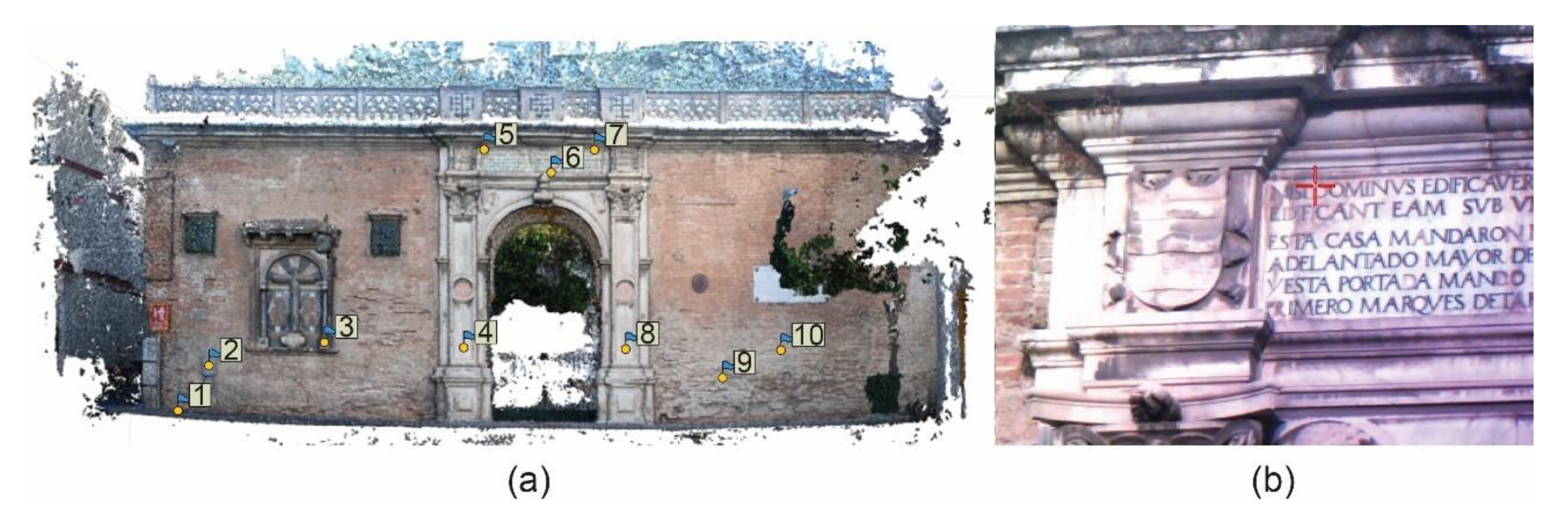
3.1. Case Study: The Main Façade of Casa de Pilatos

Casa de Pilatos is a palace located in the historic centre of Seville (Spain), whose orientalist architectural features and decorative elements (Figure 1) are in Mudejar, Gothic and Renaissance styles—the traditional Sevillian architecture from the early 16th century. The building is inspired by the Real Alcázar in Seville, particularly by the Palace of King Don Pedro, whose influence is evident in the inscriptions on its gypsum friezes [34]. One of the most remarkable spaces in the palace is the main courtyard because of its rich architectural shapes: the decoration of the arches, the Genoese marble columns imported by Don Fadrique, and the window openings to the courtyard on the ground floor, with pseudo-Nasrid columns dating from 1861 [35]. The main gate was built on an old wall (see Figure 1), including a central semicircular arch between the Corinthian pilasters erected on high bases, which were popular in Tuscany and Lombardy in the second half of the 15th century; according to Lleó Cañal [35], Don Fradrique saw this style during his trip to Italy. An 18th-century Gothic tracery balustrade, which replaces the original one, constitutes the decorative details of the top. Thus, most of the architectural details were copied from the Italian architecture of that period. This façade was chosen because of its uniqueness, since it alternates flat brick canvases with marble pilasters and an openwork crest.

3.2. Data Collection

The geometrical design seeks effective methods to visualize and, if necessary, modify the geometrical representations of solid shapes [37]. Thus, construction representations are suitable to build and transform models using high-level engineering parameters, such as distances, angles, radii and coordinate systems. For this reason, architecture makes use of spatial measurement systems. In this work, three survey methods were used: (1) traditional range survey techniques, e.g., laser meter and tape meter; (2) TLS and total station and (3) photogrammetry using a reflex camera. Short-range digital photogrammetry measures directly from photos captured at close range. The model is based on the central perspective projection and the coordinate system is arbitrarily placed in the object space, and instead the origin is located in the center of the perspective camera. The methods have been defined numerous times [38,39,40] and defined in detail the parameters camera calibration, resection, intersection and coplanarity [41]. TLS is the most widely used data acquisition technique today. It differs from the Laser Imaging Detection and Ranging (LIDAR) since it operates on an airborne platform. Its methodology is based on calculating the distance between the laser and the object. This procedure is developed using the time-of-flight method or through the transmitted and received wave of the signal [42]. The method performs a sweep of the entire surface capturing thousands of points in a coordinate system (x, y, z), obtaining the range cloud. The classic measurements were used to compare the wall thicknesses with TLS data, which were captured using a Leica ScanStation C10 [43]. Although this laser scanner had a 4-Megapixel embedded camera to map colors onto the point cloud data, a NCTech Istar [44] camera was used because of its higher resolution and HDR imaging.
On the other hand, a Leica Flexline TS02 total station with 2 mm accuracy [45] was used to record the coordinates of the GCPs on the façade. Furthermore, a Leica Disto S910 laser distance meter was used as an auxiliary piece of equipment. Its ±1.00 mm accuracy and 0.5 m in 300 m make it usable in research works [46,47]. Ten control points spread out on the façade were recorded (see Figure 2). These points should be identifiable in the subsequent photographs for SfM. GCPs above 2 m high were recorded on the upper frieze by means of natural targets.
Several devices were used in the photogrammetric survey: two Canon Digital Single Lens Reflex (DSLR) cameras producing RAW files, and a Canon E600D, an E650D and a Nikon D80 reflex camera (NEF files). The sensor of the cameras has 12 Megapixels (4000 by 3000 pixels). The main specifications of the cameras are described in Table 1. The Ground Sample Distance (GSD) represents the resolution and the detail of the final 3D reconstruction [48]. When images are not perpendicular, the GSD should be corrected using the formulae given by Leachtenauer and Driggers [49]. The effective pixel size may vary due to the lens distortion, but, as these images are not intended to perform a detailed mapping, the nominal GSD was considered [50]. Recent studies [10] determined the importance of the GSD on the accuracy of an UAV recording, for which the flight altitude is a key factor in the quality of results. In this regard, the distance was not fixed in the SfM survey. The average distance was 9 m for simple captures and 12 m for stereoscopic captures. Based on the work by Gonçalves and Henriques [50], the GSD and a fixed focal distance of 18 mm, the values 4.07 and 5.42 mm were obtained. According to these authors, the effective pixel size may be different due to the lens diffraction. The Darktable [51] open-source software was used to develop the photographs. The values for white balance, sharpness, contrast, brightness [52] and illumination parameters were adjusted. Moreover, Agisoft Metashape [53] was used for the image processing to produce 3D models from oriented and scaled images with random control points. Agisoft PhotoScan, on the other hand, processes the images through mathematical algorithms on 3D shapes [54]. Although a full description of the SfM methods is not the purpose of this paper, as [55] described them in detail, Table 2 includes the configuration parameters used in this study. This program has a simple interface and allows textured meshes and the DSM to be generated from point clouds [56].
To cover the whole width, GCPs were collected using the total station from a single position at the centre of the façade. The coordinate system was established with the axes parallel and perpendicular to the façade at 12 m. The XYZ coordinates set were 100, 100 and 10 m. The coordinates of the elements on each space were later recorded to achieve a uniform set of points. The methodology was divided into four phases. First, a test bench was chosen and survey data were collected. This test bench determined the variable geometry of the objects in the façade. As the dimensions of the case study were 20.50 m wide by 9.02 m high, short range distances were assessed [57]. Ten test datasets were carried out by varying the layout and the number of photographs. Figure 3 shows the number and the position of the cameras, and Table 3 includes the photogrammetric data. Four photograph series were taken using a single Nikon D80 SLR camera on a tripod with a nominal height of approximately 1.50 m (column 1 in Figure 3). Nadir and oblique images were taken indistinctly (up and down). Three stereoscopic series were recorded using two identical E600D and E650D reflex cameras on a single tripod with a wooden platform separated by 80 cm, considering only nadir images (column 2 of Figure 3). Other three stereoscopic series were recorded using a Nikon D80 SLR camera on a tripod with an aluminum video stabilizer sliding rail base (column 3 in Figure 3). The total width of the stabilizer was 80 cm. These last three photographic series were taken in five shots: (1) both extremes, (2) the central area and (3) two at one third. Concerning the orientation: (1) with nadir and oblique shots, (2) nadir and (3) nadir and oblique in fewer photographs and only taking central, left and right positions. The distribution of the imaging networks described in Figure 3 determines the position of the cameras in a space (x,y). To guarantee various imaging scenarios, a layout point cloud was established with different uniformity parameters and imaging distribution. Thus, researchers could know the best position in the application of façades of heritage buildings and their correlation between the number of images, capturing method, and position.
Agisoft Metashape produced dense point cloud data in a 3D coordinate system to represent the external surface of the object. An organoleptic analysis determines the distribution of the points in the space, the absence of them and the coplanarity of the segmented subset. The file formats were .e57, .ply., .xyz and .csv. The number of photographs and reprojection errors (in pixels) of the datasets were recorded. Table 3 presents the point cloud distribution, the ground resolution and the point density.
The second phase consisted of evaluating the ten photogrammetric datasets through mathematical analysis to ascertain the point density and the point cloud spatial resolution. Then, the accuracy of the entire façade between the photogrammetric series was quantitatively compared with the TLS point cloud. The fourth phase aimed at evaluating a mesh geometric pattern with the results of the previous SfM series by choosing Agisoft Metashape as the image processor. For this purpose, various applications were tested to verify the most suitable software to fit the geometry. The results were analyzed using the software chosen for the other tests. Considering the importance of DSMs, the metric accuracy of their profile as a representative standard was evaluated. Finally, following a mathematical approach, the influence of the SfM variables (the distance, the number of images, and the procedure, among others) on the results is discussed by estimating the surface deviation between the PhotoScan point set and the TLS data.

3.3. Validation of the Geometrical Pattern

After importing the SfM survey images, Agisoft Metashape performs an automatic calibration process in accordance with the exchangeable image file format (EXIF) [58] detected in the images. The process was described by Westoby et al. [59], from photo alignment to post-processing with mesh generation. On the other hand, the Metashape software has its own geometric reconstruction algorithm [60,61] and offers several levels of density of the 3D mesh. This research used the ‘high’ density level. After obtaining the dataset, various applications were tested to evaluate the quality of the 3D mesh geometry, which was later used to compare the variables from the ten surveys. Most software generate 3D meshes from TLS or SfM point clouds, such as MeshLab, Rhinoceros [62], CloudCompare [63] and Grasshopper [64], among others. Antón et al. [65] tested different commercial and open-source software to generate representative 3D meshes of the heritage assets studied in the Real Alcázar in Seville (the Pavilion of Charles V) and in the Basilica of the Baelo Claudia [66] archaeological ensemble in Tarifa, Cádiz (Spain). After a thorough accuracy and geometry evaluation of the 3D meshes, the Rhinoceros Mesh Flow plug-in [67] and the screened Poisson surface reconstruction algorithm [68] in CloudCompare provided valid results for the as-built digital reconstitution of heritage assets in HBIM.
Creating a surface mesh from a point cloud is a complex process if significant roughness is desired because of occlusion [69]. As described by Koutsoudis et al. [70], SfM methods require a large amount of memory and equipment to process field work data. In this regard, the 3D reconstruction of the façade required high performance equipment. The 3D meshing process was conducted through a dense multiple reconstruction algorithm [61]. To achieve the modeling included in Figure 4a, several steps such as those appearing in similar publications [56,59] were performed. The work was segmented into two parts to simplify the analysis. The first part focused on the base of the left pilaster (Figure 4) to analyze the geometry of the objects. On the other hand, the second part was intended to work with the commemorative plaque in the strip of the right canvas, for which the spatial resolution and point density were analyzed. Regarding the analysis of the geometry, current reconstruction algorithms smooth the surfaces if there are no points in the object. This aspect could be observed in the moldings that shape the base of the pilaster. A representative point region of the model was used for the evaluation: the section Ϡ represented in the model of Figure 4a.

4. Results and Discussion

The accuracy of SfM photogrammetric techniques is widely studied in various modalities. The accuracy and resolution of the 3D model in close-range terrestrial photogrammetry depends on several factors [57], including the distance from the camera to the façade, lens and atmospheric conditions that can alter the sharpness of photographs (e.g., fog). Poropat [71] carried out precision estimates in 95-meter and 150-meter works that showed differences between the software and the theodolite data of 0.005% and 0.02%, which are consistent experimental values in relation to theoretical expectations. Bevilacqua et al. [72] stated that the accuracy increase is linked to the base–depth relationship, the use of convergent images, and the increase in the number of points measured per image. The greater the number of images in which the same point appears, the better the accuracy. However, most studies on accuracy focus on the numbers of GCPs. Agüera et al. [28] analyzed the influence of the number of GCPs used for georeferencing on DSMs and orthoimage accuracies obtained using UAV-photogrammetry. The study showed that both horizontal and vertical accuracies increased as the number of GCPs increased. On the other hand, most studies based on the Root-Mean-Square (RMS) differentiated between GCP data and orthoimage markers for the (x,y) axis and the DSM for the z axis. Aicardi et al. [73] worked with various software to establish the accuracy between GCP data and orthophotographs. A similar work by Peña-Villasenín et al. [74] determined the accuracy of the camera arrangement on various façades. Sanz-Ablanedo et al. [10] correlated the Root-Mean-Square-Error (RMSE) with the GCPs for UAV.
Thus, many experimental DSM construction studies have evaluated the accuracy of the model. The DSM from photogrammetric surveys and the TLS reference model have been compared by evaluating the average deviation between these sources of points [7,15,75]. In contrast, Gkintzon et al. [24] discussed the reliability of the DSM and placed it at lower levels than orthophotographs and drawings–paintings, thus reconsidering the DSM as the approach to represent the geometry. Hence, the accuracy of the DSM was evaluated. The geometry from series 4 was first built to evaluate its deviation against the profile created from the TLS data. The metric variations represented in Figure 5 ranged from the pilaster floor level to approximately 1.57 m height. The average variation was therefore analyzed along the artifact, as Moyano et al. [14]. The average value yielded errors (ΔZ), and the simple absolute deviation (Dx) was calculated as per Equation (1). The results are shown in Table 4.
D x ¯ = i = 1 N xi x ¯ N
where (Dx) is the simple absolute deviation, N is the sample size, x accounts for the observed values and X is the average value of the sample (in meters).
The results showed a maximum curve dispersion of 0.0196 m between the TLS (black curve) and DSM (green curve) profiles, and an average difference of 0.0017 m. Figure 5 compares the difference between the two samples. The average value yielded errors (ΔZ) of 0.0038 m, and the simple absolute deviation (Dx) was 0.00171 m. These values represented a dispersion between the reliable model and the DSM (Figure 6) that could make the work with DSM less reliable when optimizing the accuracy in the object geometry.

4.1. Point Cloud Spatial Resolution

Point density is one of the parameters that determines the quality of the geometry of a 3D mesh when it is consistent and accurate with the geometry of the objects represented. The spatial resolution of point clouds has been scarcely determined. Peña-Villasenín et al. [74] analyzed the point density per square meter in four case studies of photogrammetry. The point density was therefore evaluated according to the surface area. The Metashape software reports the results after building the mesh model. Nevertheless, the best way to verify the point cloud spatial resolution, i.e., the 3D Euclidean distance (see Equation (2)) between the closest points, is to sample the point set.
d E P 1 , P 2 , P 3 = x 2 x 1 2 + y 2 y 1 2 + z 2 z 1 2
where d E is the Euclidean distance between points in space, and x, y and z are the Cartesian coordinates of those points.
A 70 × 70 cm2 sample of the point cloud was segmented (Figure 7) to be subsampled using CloudCompare (C2C). The flatness of this subset was approximately absolute.
Figure 8 shows the point cloud dispersion error of the ten surveys carried out at maximum, minimum and average distances from the subset. The point density was measured per square centimeter.
Survey 4 had the lowest distance values for the first, second and third quartiles of its distribution, and the lowest interquartile range. Using survey 4 as a reference for the distribution with the lowest distance between points, surveys 3, 5 and 8 obtained distributions with a low distance between points. In this regard, the values in the first and third quartiles increased with respect to survey 4: between 0.19 and 0.84 cm in survey 3, from 0.10 to 0.52 cm in survey 5 and from 0.26 to 1.21 cm in survey 8. Likewise, survey 6 yielded distributions with similar variations (between 0.26 and 0.58 cm for the distribution quartiles). However, outliers above 10 cm were detected in survey 6, which represented an excessive distance between points. In this regard, the other surveys produced outliers that showed a high distance between the points, although survey 2 obtained low values in the first quartile. Likewise, tests such as survey 1 showed high values in the first quartile, which represented high distances between the points of the element analyzed. These results implied that the number of shots and the density of points are not clearly related. Survey 4 obtained the smallest distance between points, although its low number of shots (79) was lower than those taken in survey 8 (135) and survey 10 (81). As surveys 8 and 10 were carried out on a tripod with an aluminum video stabilizer sliding rail base and survey 4 on a tripod with a nominal height of approximately 1.50 m, the number of shots and the camera positioning technique of survey 4 could be related, thus entailing better resolution of the digitized elements.

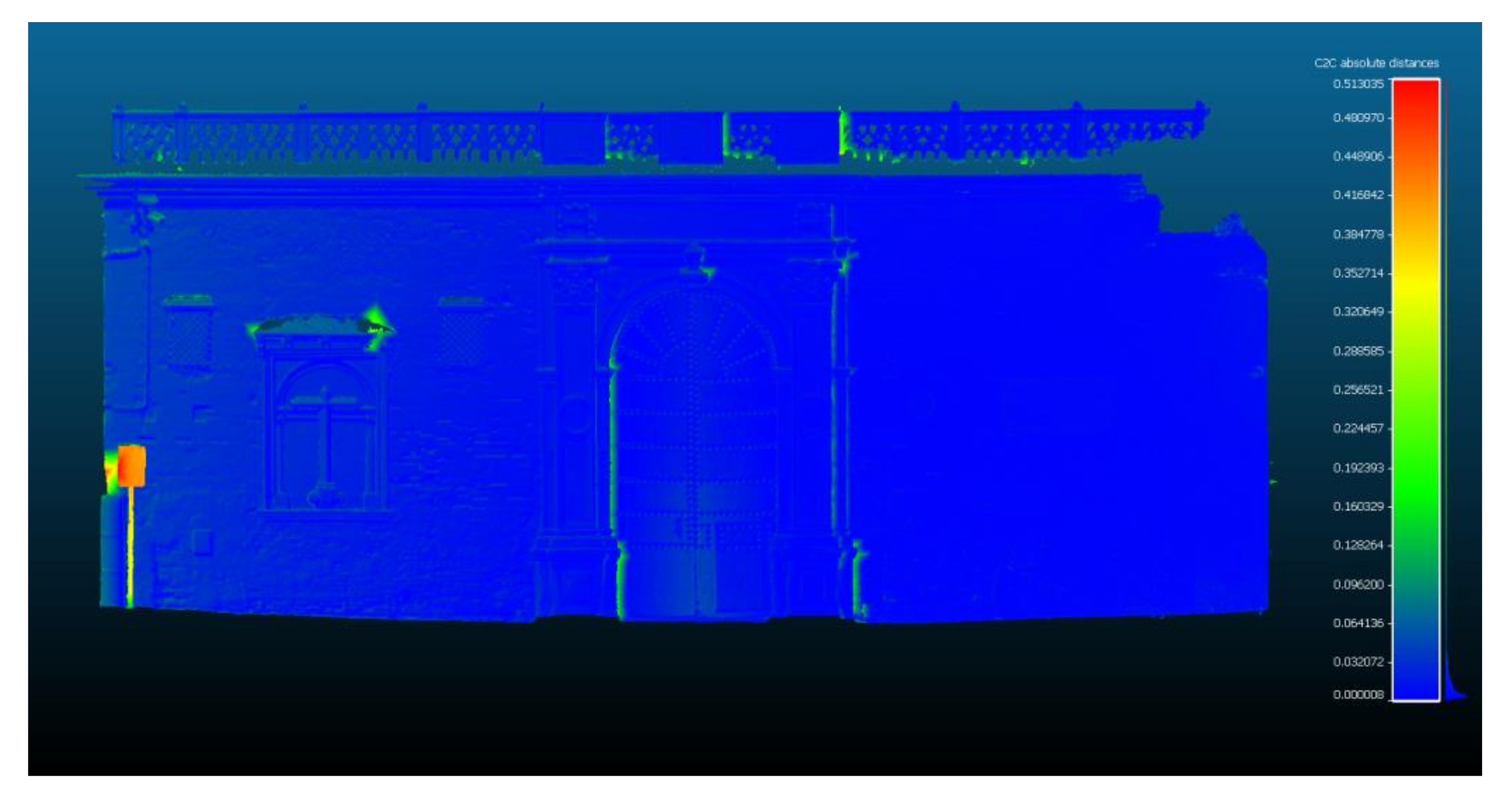
4.2. Comparison with TLS

To quantitatively compare the accuracy of the entire façade between the photogrammetric series, the TLS point cloud was taken as a reference. Once the SfM point cloud data was obtained and previously scaled with the measurements taken in Agisoft PhotoScan software, the TLS point cloud was aligned with the TLS data by selecting pairs of common points between these two point clouds in CloudCompare. The four point pairs were located at the four extreme points of the commemorative plaque, with average RMS errors of 0.01506 m. Next, the alignment was improved using the Iterative Closest Point (ICP) algorithm in CloudCompare, which was based on searching pairs of adjacent points in the two datasets to calculate the transformation parameters between them [76,77]. The RMS is stated in Table 4. Cloud-to-cloud distance computing in CloudCompare was also performed. Figure 9 shows the data capture deviation between TLS and survey 4 (in this case, taken as an example).
Georgantas et al. [78] used TLS as the reference to compare the photogrammetric IBM through C2C. Koutsoudis et al. [70] analyzed mean distances and standard deviations of all single-view range scans compared with the PhotoScan mesh. Morgan et al. [79] compared various photogrammetry applications with the TLS in laboratory on sediments with different granulometry. Thus, this method has been approved by the scientific community.
Figure 9 shows the histograms between the X, Y and Z point pairs of the photogrammetric survey 4 and the TLS point cloud as a subsample of the complete façade. The X-axis represented the intervals of distances in meters between the SfM and TLS points, whereas the Y-axis showed the point set in each interval. Variations above 82% exceeded 0.029 m. This means that 80.57% of the point pairs were matched at less than 2.9 cm using the C2C comparison algorithm, and 99.99% of the point pairs were matched at less than 1.2 cm using the M3C2® comparison algorithm created by Lague et al. [69]. The results from all series are gathered in Table 4, where surveys 3, 4 and 5 show the best results, with RMS values of 0.019, 0.026 and 0.042 m, respectively. In contrast, the other surveys were more disperse, e.g., survey 9 had a value of 0.168 m. The dataset yielded consolidated values (Figure 10). The application of the TLS and SfM in the same building allowed the point clouds recorded using quantitative data (standard deviation) to be evaluated.

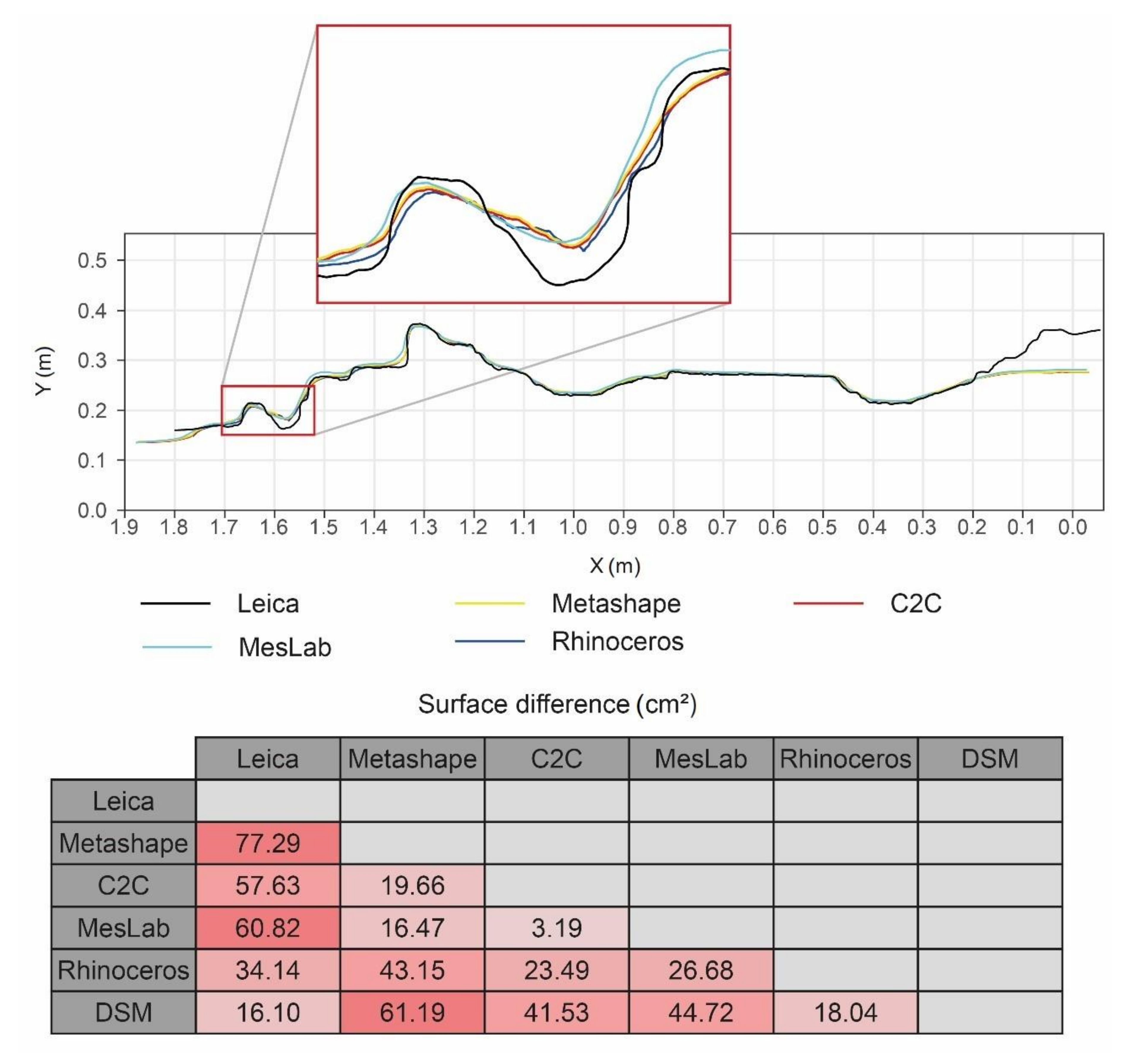
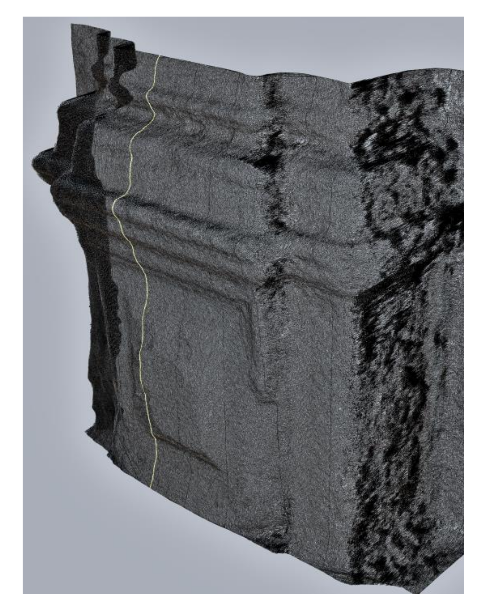
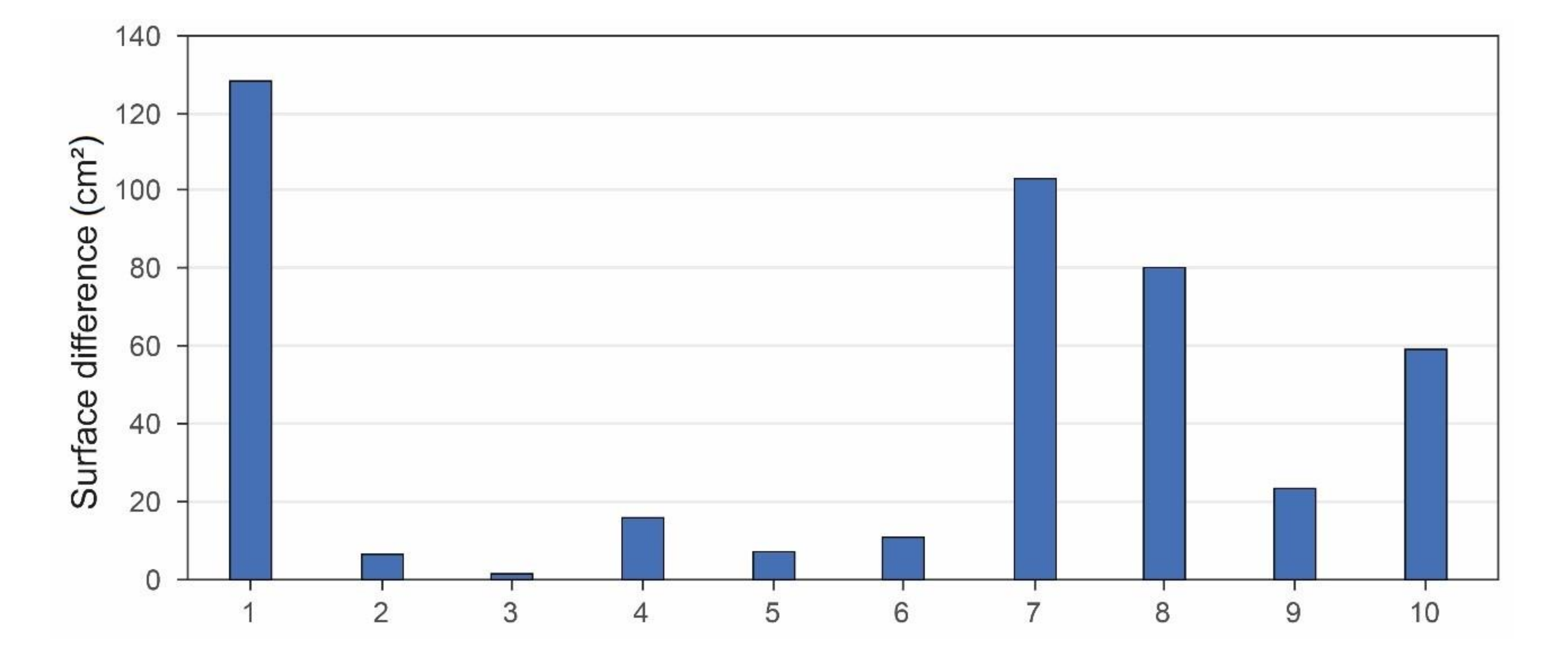
4.3. Model Geometry Analysis

Few studies have evaluated quantitatively the profiles of the textured 3D meshes from photogrammetry. Chiabrando et al. [80] established qualitative comparisons from sections generated by 3D ReShaper and radiometric sections through ESRI ArcMap. Nevertheless, profiles are important to analyze geometries and geometrical patterns in architectural objects [81]. The matching of 3D curves (one or more) with 3D surfaces was conducted by Gruen and Akca [26] with the mathematical formula. In this paper, the profiles were arranged perpendicular to the façade plane and the corresponding element at the same distance from one side of the pilaster, which means that there were geometrical constraints that made them coincide. Although a minor value of uncertainty could be estimated, it could be negligible for these geometrical values. To determine the difference between the accuracy of the 3D meshes depending on the software used, the RMS mathematical expression was used to calculate the profiles shown in the graph included in Figure 11. The difference between TLS (Leica ScanStation C10) and DSM was 1.61 mm. There was a slight difference between the geometric profiles generated by CloudCompare (C2C) and MeshLab as both used the same Poisson algorithm [68,82,83]. This accuracy was clear when reaching values of 0.31 mm, which was virtually negligible. Despite slight fluctuations in the curve, the Rhinoceros was the most stable application within the whole. This program showed variations that ranged from 2 to 4 mm with respect to the others. Metashape provided the most disperse results when generating the 3D mesh. The difference with the pattern was 7.72 mm. Compared to a uniform mesh that fits the minimum triangles, a scattered mesh and a non-uniform triangulation outcome can be observed, so this mesh was not representative of the minimum density of the point cloud. As regards the triangulation in the areas where the point density decreased, the software lengthened the triangle (vertexes displacement).
The variation between the profile shown by the TLS point cloud and that of the meshes generated by various algorithms in the evaluation of survey 4 was significant in some cases. Slight variations of 1 mm were detected, except in two regions, with variations of 10 mm (curve at 1.35 mm and 1.55 mm of elevation). The SfM series 4 was used for this validation study. Either the C2C or the MeshLab geometry could be used as both are the most uniform software and do not experience large variations. A debate could be based as to whether it would be more appropriate to compare the point cloud in an object profile environment, as in the study by Barba et al. [84], in comparison with the reprojection error. These authors believed that the purpose of information records is to generate 3D models, and therefore the best way to evaluate their accuracy is through this process, despite the fact that generated profiles of the dense cloud are mostly used. On the other hand, according to Remondino et al. [8], the accuracy would be established by a flatness error if the profile is generated from the point cloud.
Based on the results that determined the most reliable software, and considering that the sample of the TLS profile was representative, the photogrammetric surveys were compared. The 3D meshing process was performed with the Rhinoceros ‘MeshPatch’ command to create a section of the object using the Ϡ plane, as shown in Figure 12.
The subsets of the closest points in a x,y coordinate system were extracted from the mesh profiles. The values obtained as per Equation (3) are represented in the following barplot (Figure 13).
A = f x dx g x dx
where A is the differential area between the curves, and f x dx and g x dx are their functions.
Rhinoceros software was used to section the 3D meshes using the Ϡ plane to create the profiles from which the points for the accuracy calculation of the series were extracted.
Table 4 was shown as the differential area between the base profile from the TLS data and the other profiles according to the representative sample of the subset of points in each survey. The area is expressed in square centimeters. Thus, series 3 was the most suitable value within the dataset, with 1.15 cm2 along the section profile, whereas series 1 and 7 obtained the worst results: 128.01 cm2 and 103.34 cm2, respectively. Figure 13 shows that series 3, 2 and 4 obtained the lowest values (apart from survey 6) and the best shots distribution, distances and number. Accordingly, the number of photographs influenced the accuracy. The geometric quality and point coincidences on the pilaster base was greater in series 3 with only 44 photographs than in series 4, which was dispersed and included nadir and oblique photographs (Figure 3). Regarding the planning to acquire the photographs and the distances to the façade plane, series 3 and 4 had the same average length. As for this parameter, series 5, 6 and 7 were the most distant photographs; however, the results were different. The three stereoscopic series with simultaneous cameras also obtained suitable results, except for series 7 whose number of photographs was lower. The stereoscopic block with rail and a single camera produced uneven results as in survey 8, despite its 135 shots. Better results were expected to evaluate this new procedure of alternating nadir and oblique cameras in minor sequences.
McCarthy [85] stated that many studies [78,86,87] have demonstrated that multi-image photogrammetry can achieve results close or even superior to those from the TLS, always under the right conditions. This research proved that the difference between the DSM of a series (e.g., series 4) and the digital model generated from the point cloud of TLS data was approximately 1.7 mm. The 3D digital model from the TLS point cloud properly conformed to the overall geometry of the architectural shapes, including the subtle details of the vertical moldings (Figure 14). The SfM of the most accurate series, in the absence or decrease in points density when meshing, produced shapes millimeters away from the physical reality of the object.
The sample used as a reference to compare the photogrammetric samples was the TLS data. The geometry evaluation revealed that the profiles generated by the photogrammetric surveys significantly varied in the regions of points perpendicular to the camera. The reason was the inefficacy of the SfM software in the reconstruction because there were no oblique photographs. However, the 9 mm accuracy could be acceptable at the 1:50 scale, as established by the English Heritage guidelines? Regarding scale tolerance and point density [88], the maximum tolerance required for the precision of detail for scale 1:50 should be ±15 mm. Considering the density of each series and the guidelines mentioned above, survey 9 showed poor precision, and surveys 9, 1 and 7 showed poor point density.
Although this research showed suitable results of interpolation between PD density of TLS points and the photogrammetry in series 4, this test 4 is not always the best in the geometry evaluation. Therefore, this is a new open field between the results of affinity, the point density and the geometry analysis that should be validated in further studies.

5. Conclusions

One of the current issues is the reverse engineering process for HBIM, i.e., to generate a parametric 3D model from point cloud data to include the deformations and geometric peculiarities of heritage assets [65]. This research showed that photogrammetry, together with a topographic instrument, could constitute an interesting technical and economic reality. This study focuses on the accuracy between TLS and SfM, shows that photogrammetry is a suitable technique for dense 3D cloud reconstruction, and, by studying the accuracy of DSMs, assesses the point cloud geometry for the SfM geometric reconstruction of 3D architectural and archaeological objects. Thus, this study analyzed the distribution of imaging networks suitably placed in a space (x,y) to analyze a façade plane. Moreover, the difference between the capture of simple and stereoscopic images was introduced. These procedures originated various surface models where the geometric quality of the 3D results was evaluated, an aspect not studied up to now.
The point density and geometry analyses for SfM revealed how photogrammetric series should be addressed. For this purpose, low-cost elements were used, which could produce a huge advantage as in the case of stereoscopic pair shots.
In contrast to other studies, the number of photographs did not always determine an appropriate dataset, unless the survey was properly planned. In relation to the precision studies on DSM, there is a large deviation in the 3D mesh in comparison with the meshing process of the Metashape software. To obtain a good dataset, the taking of photographs disorderly distributed in the façade plane of the building should be planned. Most surface should be covered. The better the uniformity in the distances to the plane, the better are the results.
This paper is a first approach to study the accuracy that SfM can provide BIM with, thus opening a new paradigm in the use of low-cost tools in modeling. To corroborate this affirmation, medium resolution reflex cameras (compared to current cameras) were used in the experimentation, together with a Laser Leica Disto TM S910 equipment, which is cheaper than topographic equipment, such as Leica Flexline TS02 total station with 2 mm accuracy. However, Laser Leica Disto TM S910 also limits the accuracy in large lengths.
The photogrammetric process has so far used sequences of unordered images, but this research revealed that photographs should be distributed along the surface to be surveyed to achieve a suitable point density and geometry. Therefore, photogrammetric surveys using a single camera and less than 45 shots are not advisable: they should be nadir and oblique for 181.35 m2.
Today, sequences of stereoscopic photographs with the new instruments improve the results of close-range photogrammetry, requiring fewer shots. Despite the 135 shots of survey 8, for instance, the stereoscopic block with rail and a single camera produced uneven results, although better results were expected to evaluate this new procedure of alternating nadir and oblique cameras in minor sequences. The reason could be the consequence of uneven positioning (scarce dispersion) of the tripod along the façade width.
This study stresses that, based on a series of imaging networks taking through the photogrammetric technique, the accuracy of the techniques to acquire point cloud data by means of DSM is assessed. The impact relies on the fact that many research studies on this area use DSM as the model to compare the quality of the 3D representation, so researchers have a reference on the variation of the model.
As is well known in the scientific community, the methods based on photographs imply many steps, each with a certain algorithm. Each parameter could obtain various results, so this aspect will be further studied. In addition, the results could be improved by using different lens and sensors and by improving the calibration parameters, so this new challenge could be considered in the future.

Author Contributions

Conceptualisation, J.M.; Methodology, J.M., and J.E.N.-J.; Software, J.M., and J.E.N.-J.; Validation, J.E.N.-J.; Formal Analysis, D.M.-G.; Investigation, J.M. and D.B.-H.; Resources, J.M.; Data Curation, Writing—Original Draft Preparation, J.M., D.M.-G., and D.B.-H.; Writing—Review & Editing, J.M., D.M.-G., and D.B.-H.; Visualisation, D.M.-G., and J.E.N.-J.; Supervision, J.M., and D.B.-H.; Project Administration, J.M.; Funding Acquisition, J.M. All authors have read and agreed to the published version of the manuscript.

Funding

This research was funded by Universidad de Sevilla through VI Plan Propio de Investigación y Transferencia (VIPPIT).

Acknowledgments

Thanks to the Administration of Casa de Pilatos for providing access to the building.

Conflicts of Interest

The authors declare no conflict of interest. The funders had no role in the design of the study; in the collection, analyses, or interpretation of data; in the writing of the manuscript, or in the decision to publish the results.

Abbreviations

The following abbreviations are used in this paper:
TLSTerrestrial Laser Scanning
SfMStructure-from-Motion
MDCSMassive Data Capture Systems
UAVsUnmanned Aerial Vehicles
DSMsDigital Surface Models
ICOMOSInternational Council on Monuments and Sites
ISPRSInternational Society for Photogrammetry and Remote Sensing
BIMBuilding Information Modeling
HBIMHistoric Building Information Modeling
GCPsGround Control Points
DBATDamped Bundle Adjustment Toolbox
RPASRemotely Piloted Aircraft Systems
DSLRDigital Single Lens Reflex
HDRHigh Dynamic Range
RMSRoot-Mean-Square
RMSERoot-Mean-Square-Error
MVSMulti-view Stereo
EXIFExchangeable image file format

Symbols

The following symbols are used in this paper:
d E Euclidean Distance
wSensor width
WPhotograph width
HDistance from camera to object
σStandard deviation
nSample size
x, yObserved values
x ¯ Mean value

References

  1. Hambly, M. Drawing Instruments, 1580–1980; Sotheby’s Publications by Philip Wilson Publishers Ltd.: London, UK, 1988. [Google Scholar]
  2. Bork, R. The Flowering of Rayonnant Drawing in the Rhineland. In The Geometry of Creation Architectural Drawing and the Dynamics of Gothic Design; Routledge: Abingdon-on-Thames, UK, 2011; pp. 56–165. [Google Scholar]
  3. Sansoni, G.; Trebeschi, M.; Docchio, F. State-of-The-Art and Applications of 3D Imaging Sensors in Industry, Cultural Heritage, Medicine, and Criminal Investigation. Sensors 2009, 9, 568–601. [Google Scholar] [CrossRef] [PubMed]
  4. Bruno, S.; De Fino, M.; Fatiguso, F. Historic Building Information Modelling: Performance assessment for diagnosis-aided information modelling and management. Autom. Constr. 2018, 86, 256–276. [Google Scholar] [CrossRef]
  5. Omar, T.; Nehdi, M.L. Data acquisition technologies for construction progress tracking. Autom. Constr. 2016, 70, 143–155. [Google Scholar] [CrossRef]
  6. Rönnholm, P.; Honkavaara, E.; Litkey, P.; Hyyppä, H.; Hyyppä, J. Integration of laser scanning and photogrammetry. Int. Arch. Photogramm. Remote Sens. Spat. Inf. Sci. 2007, 36, 355–362. [Google Scholar]
  7. Cardaci, A.; Mirabella Roberti, G.; Versaci, A. The integrated 3d survey for planned conservation: The former church and convent of Sant’Agostino in Bergamo. ISPRS-Ann. Photogramm. Remote Sens. Spat. Inf. Sci. 2019, 42, 235–242. [Google Scholar] [CrossRef] [Green Version]
  8. Remondino, F.; Spera, M.G.; Nocerino, E.; Menna, F.; Nex, F. State of the art in high density image matching. Photogramm. Rec. 2014, 29, 144–166. [Google Scholar] [CrossRef] [Green Version]
  9. Colomina, I.; Molina, P. Unmanned aerial systems for photogrammetry and remote sensing: A review. ISPRS J. Photogramm. Remote Sens. 2014, 92, 79–97. [Google Scholar] [CrossRef] [Green Version]
  10. Sanz-Ablanedo, E.; Chandler, J.; Rodríguez-Pérez, J.; Ordóñez, C. Accuracy of Unmanned Aerial Vehicle (UAV) and SfM Photogrammetry Survey as a Function of the Number and Location of Ground Control Points Used. Remote Sens. 2018, 10, 1606. [Google Scholar] [CrossRef] [Green Version]
  11. Martínez-Carricondo, P.; Carvajal-Ramírez, F.; Yero-Paneque, L.; Agüera-Vega, F. Combination of nadiral and oblique UAV photogrammetry and HBIM for the virtual reconstruction of cultural heritage. Case study of Cortijo del Fraile in Níjar, Almería (Spain). Build. Res. Inf. 2019, 48, 140–159. [Google Scholar] [CrossRef]
  12. Guarnieri, A.; Milan, N.; Vettore, A. Monitoring Of Complex Structure For Structural Control Using Terrestrial Laser Scanning (Tls) And Photogrammetry. Int. J. Archit. Herit. 2013, 7, 54–67. [Google Scholar] [CrossRef]
  13. Nieto-Julián, J.E.; Antón, D.; Moyano, J.J. Implementation and Management of Structural Deformations into Historic Building Information Models. Int. J. Archit. Herit. 2020, 14, 1384–1397. [Google Scholar] [CrossRef]
  14. Moyano, J.; Odriozola, C.P.; Nieto-Julián, J.E.; Vargas, J.M.; Barrera, J.A.; León, J. Bringing BIM to archaeological heritage: Interdisciplinary method/strategy and accuracy applied to a megalithic monument of the Copper Age. J. Cult. Herit. 2020, 45, 303–314. [Google Scholar] [CrossRef]
  15. Bolognesi, M.; Furini, A.; Russo, V.; Pellegrinelli, A.; Russo, P. Accuracy of cultural heritage 3D models by RPAS and terrestrial photogrammetry. Int. Arch. Photogramm. Remote Sens. Spat. Inf. Sci. ISPRS Arch. 2014, 40, 113–119. [Google Scholar] [CrossRef] [Green Version]
  16. Rebolj, D.; Pučko, Z.; Babič, N.Č.; Bizjak, M.; Mongus, D. Point cloud quality requirements for Scan-vs-BIM based automated construction progress monitoring. Autom. Constr. 2017, 84, 323–334. [Google Scholar] [CrossRef]
  17. U.S. General Services Administration. GSA Building Information Modeling Guide Series: 03; U.S. General Services Administration: Washington, DC, USA, 2009.
  18. Dai, F.; Rashidi, A.; Brilakis, I.; Vela, P. Comparison of image-based and time-of-flight-based technologies for three-dimensional reconstruction of infrastructure. J. Constr. Eng. Manag. 2013, 139, 69–79. [Google Scholar] [CrossRef]
  19. Akca, D.; Freeman, M.; Sargent, I.; Gruen, A. Quality assessment of 3D building data. Photogramm. Rec. 2010, 25, 339–355. [Google Scholar] [CrossRef] [Green Version]
  20. Khoshelham, K.; Elberink, S.O. Accuracy and Resolution of Kinect Depth Data for Indoor Mapping Applications. Sensors 2012, 12, 1437–1454. [Google Scholar] [CrossRef] [Green Version]
  21. Kinect, W.S.D.K. Download Kinect for Windows SDK v1.8 from Official Microsoft Download Center. Available online: https://www.microsoft.com/en-us/download/details.aspx?id=40278 (accessed on 5 June 2020).
  22. Agüera-Vega, F.; Carvajal-Ramírez, F.; Martínez-Carricondo, P. Accuracy of digital surface models and orthophotos derived from unmanned aerial vehicle photogrammetry. J. Surv. Eng. 2017, 143, 04016025. [Google Scholar] [CrossRef]
  23. Mesas-Carrascosa, F.; Rumbao, I.; Berrocal, J.; Porras, A. Positional Quality Assessment of Orthophotos Obtained from Sensors Onboard Multi-Rotor UAV Platforms. Sensors 2014, 14, 22394–22407. [Google Scholar] [CrossRef]
  24. Gkintzou, C.; Georgopoulos, A.; Valle Melón, J.M.; Rodríguez Miranda, Á. Virtual Reconstruction of the ancient state of a ruined Church. In Project Paper in “Lecture Notes in Computer Science (LNCS)”, Proceedings of the 4th International EuroMediterranean Conference (EUROMED), Limassol, Cyprus, 29 October–3 November 2012; Springer: Berlin/Heidelberg, Germany, 2012. [Google Scholar]
  25. Galeazzi, F. Towards the definition of best 3D practices in archaeology: Assessing 3D documentation techniques for intra-site data recording. J. Cult. Herit. 2016, 17, 159–169. [Google Scholar] [CrossRef]
  26. Gruen, A.; Akca, D. Least squares 3D surface and curve matching. ISPRS J. Photogramm. Remote Sens. 2005, 59, 151–174. [Google Scholar] [CrossRef] [Green Version]
  27. Galantucci, R.A.; Fatiguso, F. Advanced damage detection techniques in historical buildings using digital photogrammetry and 3D surface anlysis. J. Cult. Herit. 2019, 36, 51–62. [Google Scholar] [CrossRef]
  28. Agüera-Vega, F.; Carvajal-Ramírez, F.; Martínez-Carricondo, P. Assessment of photogrammetric mapping accuracy based on variation ground control points number using unmanned aerial vehicle. Meas. J. Int. Meas. Confed. 2017, 98, 221–227. [Google Scholar] [CrossRef]
  29. Murtiyoso, A.; Grussenmeyer, P.; Börlin, N. Reprocessing close range terrestrial and uav photogrammetric projects with the dbat toolbox for independent verification and quality control. Int. Arch. Photogramm. Remote Sens. Spat. Inf. Sci. ISPRS Arch. 2017, 42, 171–177. [Google Scholar] [CrossRef] [Green Version]
  30. Russo, M.; Giugliano, A.M.; Asciutti, M. Mobile phone imaging for CH façade modelling. Int. Arch. Photogramm. Remote Sens. Spat. Inf. Sci.-ISPRS Arch. 2019, 42, 287–294. [Google Scholar] [CrossRef] [Green Version]
  31. Karachaliou, E.; Georgiou, E.; Psaltis, D.; Stylianidis, E. UAV for mapping historic buildings: From 3D modelling to BIM. ISPRS Ann. Photogramm. Remote Sens. Spat. Inf. Sci. 2019, XLII-2, 397–402. [Google Scholar] [CrossRef] [Green Version]
  32. Achille, C.; Adami, A.; Chiarini, S.; Cremonesi, S.; Fassi, F.; Fregonese, L.; Taffurelli, L. UAV-Based Photogrammetry and Integrated Technologies for Architectural Applications-Methodological Strategies for the After-Quake Survey of Vertical Structures in Mantua (Italy). Sensors 2015, 15, 15520–15539. [Google Scholar] [CrossRef] [Green Version]
  33. Pepe, M.; Ackermann, S.; Fregonese, L.; Achille, C. 3D Point Cloud Model Color Adjustment by Combining Terrestrial Laser Scanner and Close Range Photogrammetry Datasets. World Acad. Sci. Eng. Technol. Int. J. Comput. Inf. Eng. 2016, 10, 1942–1948. [Google Scholar]
  34. Bernal, A.A. El origen de la Casa de Pilatos de Sevilla. 1483–1505. Atrio. Rev. Hist. Arte 2011, 17, 133–172. [Google Scholar]
  35. Cañal, V.L. La Casa de Pilatos. Archit. Vie 1994, 6, 181–192. [Google Scholar]
  36. Hielscher, K. La Espana Incognita; Arquitectura, Paisajes, Vida Popular. Available online: https://www.iberlibro.com/buscar-libro/titulo/la-espana-incognita-arquitectura-paisajes-vida-popular/autor/kurt-hielscher/ (accessed on 12 May 2020).
  37. Prautzsch, H.; Boehm, W. Computer Aided Geometric Design. In Handbook of Computer Aided Geometric Design; Academic Press: Cambridge, MA, USA, 2002; pp. 255–282. ISBN 978-0-444-51104-1. [Google Scholar]
  38. Grussenmeyer, P.; Al Khalil, O. Solutions for exterior orientation in photogrammetry: A review. Photogramm. Rec. 2002, 17, 615–634. [Google Scholar] [CrossRef]
  39. Yilmaz, H.M.; Yakar, M.; Gulec, S.A.; Dulgerler, O.N. Importance of digital close-range photogrammetry in documentation of cultural heritage. J. Cult. Herit. 2007, 8, 428–433. [Google Scholar] [CrossRef]
  40. Arias, P.; Herráez, J.; Lorenzo, H.; Ordóñez, C. Control of structural problems in cultural heritage monuments using close-range photogrammetry and computer methods. Comput. Struct. 2005, 83, 1754–1766. [Google Scholar] [CrossRef]
  41. Yilmaz, H.M.; Yakar, M.; Yildiz, F. Documentation of historical caravansaries by digital close range photogrammetry. Autom. Constr. 2008, 17, 489–498. [Google Scholar] [CrossRef]
  42. Yastikli, N. Documentation of cultural heritage using digital photogrammetry and laser scanning. J. Cult. Herit. 2007, 8, 423–427. [Google Scholar] [CrossRef]
  43. Geosystems, L. Leica ScanStation C10—The All-in-One Laser Scanner for Any Application. Available online: http://leica-geosystems.com/products/laser-scanners/scanners/leica-scanstation-c10 (accessed on 15 January 2020).
  44. Nctech iSTAR 360 Degree Measurement Module Integrated by Imaging Companies. Available online: https://www.nctechimaging.com/istar-360-degree-measurement-module-integrated-by-imaging-companies/ (accessed on 5 June 2020).
  45. Geosystems Leica Geosystems (2008) Leica FlexLine TS02/TS06/TS09 User Manual. Available online: https://leica-geosystems.com/ (accessed on 16 March 2020).
  46. Bohorquez, P.; del Moral-Erencia, J.D. 100 Years of Competition between Reduction in Channel Capacity and Streamflow during Floods in the Guadalquivir River (Southern Spain). Remote Sens. 2017, 9, 727. [Google Scholar] [CrossRef] [Green Version]
  47. Bohorquez, P.; Del Moral-Erencia, J.D. Parametric study of trends in flood stages over time in the regulated Guadalquivir River (years 1910–2016). Proc. Eur. Water 2017, 59, 145–151. [Google Scholar]
  48. Bolognesi, C.; Garagnani, S. From a point cloud survey to a mass 3d modelling: Renaissance HBIM in Poggio a Caiano. Isprs-Int. Arch. Photogramm. Remote Sens. Spat. Inf. Sci. 2018, XLII-2, 117–123. [Google Scholar] [CrossRef] [Green Version]
  49. Leachtenauer, J.C.; Driggers, R.G. Surveillance and Reconnaissance Imaging Systems: Modeling and Performance Prediction; Artech House: Norfolk County, MA, USA, 2001. [Google Scholar]
  50. Gonçalves, J.A.; Henriques, R. UAV photogrammetry for topographic monitoring of coastal areas. ISPRS J. Photogramm. Remote Sens. 2015, 104, 101–111. [Google Scholar] [CrossRef]
  51. David, P.H. Darktable. Available online: https://www.darktable.org/ (accessed on 30 January 2020).
  52. Sieberth, T.; Wackrow, R.; Hofer, V.; Barrera, V. Light Field Camera as Tool for Forensic Photogrammetry. Isprs-Int. Arch. Photogramm. Remote Sens. Spat. Inf. Sci. 2018, XLII-1, 393–399. [Google Scholar] [CrossRef] [Green Version]
  53. Agisoft PhotoScan Software. Agisoft Metashape. Available online: https://www.agisoft.com/ (accessed on 30 January 2020).
  54. Szeliski, R. Computer Vision: Algorithms and Applications; Springer-Verlag: London, UK, 2010. [Google Scholar]
  55. Jaud, M.; Passot, S.; Allemand, P.; Le Dantec, N.; Grandjean, P.; Delacourt, C. Suggestions to Limit Geometric Distortions in the Reconstruction of Linear Coastal Landforms by SfM Photogrammetry with PhotoScan® and MicMac® for UAV Surveys with Restricted GCPs Pattern. Drones 2018, 3, 2. [Google Scholar] [CrossRef] [Green Version]
  56. Verhoeven, G. Taking computer vision aloft-archaeological three-dimensional reconstructions from aerial photographs with photoscan. Archaeol. Prospect. 2011, 18, 67–73. [Google Scholar] [CrossRef]
  57. Haneberg, W.C. Using close range terrestrial digital photogrammetry for 3-D rock slope modeling and discontinuity mapping in the United States. Bull. Eng. Geol. Environ. 2008, 67, 457–469. [Google Scholar] [CrossRef]
  58. Romero, N.L.; Gimenez Chornet, V.V.G.C.; Cobos, J.S.; Selles Carot, A.A.S.C.; Centellas, F.C.; Mendez, M.C. Recovery of descriptive information in images from digital libraries by means of EXIF metadata. Libr. Hi Tech 2008, 26, 302–315. [Google Scholar] [CrossRef]
  59. Westoby, M.J.; Brasington, J.; Glasser, N.F.; Hambrey, M.J.; Reynolds, J.M. ‘Structure-from-Motion’ photogrammetry: A low-cost, effective tool for geoscience applications. Geomorphology 2012, 179, 300–314. [Google Scholar] [CrossRef] [Green Version]
  60. Seitz, S.M.; Curless, B.; Diebel, J.; Scharstein, D.; Szeliski, R. A comparison and evaluation of multi-view stereo reconstruction algorithms. In Proceedings of the IEEE Computer Society Conference on Computer Vision and Pattern Recognition, New York, NY, USA, 17–22 June 2006; Volume 1, pp. 519–526. [Google Scholar]
  61. Scharstein, D.; Szeliski, R. A Taxonomy and Evaluation of Dense Two-Frame Stereo Correspondence Algorithms. Int. J. Comput. Vis. 2002, 47, 7–42. [Google Scholar] [CrossRef]
  62. Robert McNeel & Associates Rhinoceros. Available online: https://www.rhino3d.com/ (accessed on 24 January 2020).
  63. Girardeau-Montaut, D. Cloud-to-Mesh Distance. Available online: http://www.cloudcompare.org/doc/wiki/index.php?title=Cloud-to-Mesh_Distance (accessed on 2 May 2020).
  64. Robert McNeel & Associates Grasshopper Grasshopper. Available online: https://www.grasshopper3d.com/ (accessed on 4 March 2020).
  65. Antón, D.; Medjdoub, B.; Shrahily, R.; Moyano, J. Accuracy evaluation of the semi-automatic 3D modeling for historical building information models. Int. J. Archit. Herit. 2018, 12, 790–805. [Google Scholar] [CrossRef] [Green Version]
  66. Antón, D.; Pineda, P.; Medjdoub, B.; Iranzo, A. As-built 3D heritage city modelling to support numerical structural analysis: Application to the assessment of an archaeological remain. Remote Sens. 2019, 11, 1276. [Google Scholar] [CrossRef] [Green Version]
  67. Reverse, M. Mesh Flow. 2016. Available online: http://v5.rhino3d.com/forum/topics/mesh-flow-plug-in (accessed on 15 January 2020).
  68. Kazhdan, M.; Hoppe, H. Screened poisson surface reconstruction. ACM Trans. Graph. 2013, 32, 1–13. [Google Scholar] [CrossRef] [Green Version]
  69. Lague, D.; Brodu, N.; Leroux, J. Accurate 3D comparison of complex topography with terrestrial laser scanner: Application to the Rangitikei canyon (N-Z). ISPRS J. Photogramm. Remote Sens. 2013, 82, 10–26. [Google Scholar] [CrossRef] [Green Version]
  70. Koutsoudis, A.; Vidmar, B.; Ioannakis, G.; Arnaoutoglou, F.; Pavlidis, G.; Chamzas, C. Multi-image 3D reconstruction data evaluation. J. Cult. Herit. 2014, 15, 73–79. [Google Scholar] [CrossRef]
  71. Poropat, G.; Tonon, F.; Kottenstette, J.J. Remote 3D mapping of rock mass structure. In Laser and Photogrammetric Methods for Rock Face Characterization; American Rock Mechanics Association: Alexandria, VA, USA, 2006; pp. 63–75. Available online: https://docplayer.net/48156338-Laser-and-photogrammetric-methods-for-rock-face-characterization.html (accessed on 31 October 2020).
  72. Bevilacqua, M.G.; Caroti, G.; Piemonte, A.; Ulivieri, D. Reconstruction of Lost Architectural Volumes By Integration of Photogrammetry From Archive Imagery With 3-D Models of the Status Quo. ISPRS-Int. Arch. Photogramm. Remote Sens. Spat. Inf. Sci. 2019, XLII-2/W9, 119–125. [Google Scholar] [CrossRef] [Green Version]
  73. Aicardi, I.; Chiabrando, F.; Maria Lingua, A.; Noardo, F. Recent trends in cultural heritage 3D survey: The photogrammetric computer vision approach. J. Cult. Herit. 2018, 32, 257–266. [Google Scholar] [CrossRef]
  74. Peña-Villasenín, S.; Gil-Docampo, M.; Ortiz-Sanz, J. 3-D Modeling of Historic Façades Using SFM Photogrammetry Metric Documentation of Different Building Types of a Historic Center. Int. J. Archit. Herit. 2017, 11, 871–890. [Google Scholar] [CrossRef]
  75. Smith, M.W.; Vericat, D. From experimental plots to experimental landscapes: Topography, erosion and deposition in sub-humid badlands from Structure-from-Motion photogrammetry. Earth Surf. Process. Landf. 2015, 40, 1656–1671. [Google Scholar] [CrossRef] [Green Version]
  76. Rajendra, Y.D.; Mehrotra, S.C.; Kale, K.V.; Manza, R.R.; Dhumal, R.K.; Nagne, A.D.; Vibhute, D.; Ramanujan, S.; Chair, G. Evaluation of Partially Overlapping 3D Point Cloud’s Registration by using ICP variant and CloudCompare. Isprs Int. Arch. Photogramm. Remote Sens. Spat. Inf. Sci. 2014, XL-8, 891–897. [Google Scholar] [CrossRef] [Green Version]
  77. Moon, D.; Chung, S.; Kwon, S.; Seo, J.; Shin, J. Comparison and utilization of point cloud generated from photogrammetry and laser scanning: 3D world model for smart heavy equipment planning. Autom. Constr. 2019, 98, 322–331. [Google Scholar] [CrossRef]
  78. Georgantas, A.; Brédif, M.; Pierrot-Desseilligny, M. An accuracy assessment of automated photogrammetric techniques for 3D modelling of complex interiors. Int. Arch. Photogramm. Remote Sens. Spat. Inf. Sci. 2012, XXXIX-B3, 23–28. [Google Scholar] [CrossRef] [Green Version]
  79. Morgan, J.A.; Brogan, D.J.; Nelson, P.A. Application of Structure-from-Motion photogrammetry in laboratory flumes. Geomorphology 2017, 276, 125–143. [Google Scholar] [CrossRef] [Green Version]
  80. Chiabrando, F.; Lingua, A.; Noardo, F.; Spanò, A. 3D modelling of trompe l’oeil decorated vaults using dense matching techniques. Int. Arch. Photogramm. Remote Sens. Spat. Inf. Sci. 2014, 2, 97–104. [Google Scholar] [CrossRef] [Green Version]
  81. Moyano, J.J.; Barrera, J.A.; Nieto, J.E.; Marín, D.; Antón, D. A geometrical similarity pattern as an experimental model for shapes in architectural heritage: A case study of the base of the pillars in the Cathedral of Seville and the church of Santiago in Jerez, Spain. ISPRS-Int. Arch. Photogramm. Remote Sens. Spat. Inf. Sci. 2017, XLII-2/W3, 511–517. [Google Scholar] [CrossRef] [Green Version]
  82. Yu, Y.; Zhou, K.; Xuz, D.; Shi, X.; Bao, H.; Guo, B.; Shum, H.Y. Mesh Editing with Poisson-Based Gradient Field Manipulation; ACM SIGGRAPH 2004 Papers; ACM Press: New York, NY, USA, 2004; pp. 644–651. [Google Scholar]
  83. Kazhdan, M.; Bolitho, M.; Hoppe, H. Poisson Surface Reconstruction. In Proceedings of the fourth Eurographics Symposium on Geometry Processing, Sardinia, Italy, 26–28 June 2006; pp. 61–70. [Google Scholar]
  84. Barba, S.; Barbarella, M.; Di Benedetto, A.; Fiani, M.; Gujski, L.; Limongiello, M. Accuracy Assessment of 3D Photogrammetric Models from an Unmanned Aerial Vehicle. Drones 2019, 3, 79. [Google Scholar] [CrossRef] [Green Version]
  85. McCarthy, J. Multi-image photogrammetry as a practical tool for cultural heritage survey and community engagement. J. Archaeol. Sci. 2014, 43, 175–185. [Google Scholar] [CrossRef]
  86. Pierrot-Deseilligny, M.; De Luca, L.; Remondino, F. Automated Image-Based Procedures for Accurate Artifacts 3D Modeling and Orthoimage Generation. Geoinform. FCE CTU 2011, 6, 291–299. [Google Scholar] [CrossRef]
  87. Chandler, J.; Fryer, J. Low cost digital photogrammetry. AutoDesk 123D Catch: How accurate is it? Geomat. World 2013, 2, 28–30. [Google Scholar]
  88. Bryan, P.; Blake, B.; Bedford, J.; Barber, D.; Mills, J. Metric Survey Specifications for Cultural Heritage; English Heritage: Swindon, UK, 2009. [Google Scholar]
Figure 1. View of the main façade of Casa de Pilatos: (a) current state and (b) photograph by Kurt Hielscher [36] during his stay in Seville from 1914 to 1918.
Remotesensing 12 03571 g001
Figure 2. (a) Ground Control Points (GCPs) on the façade and (b) cross hairs pointing a natural target.
Remotesensing 12 03571 g002
Figure 3. Distribution of the imaging networks in the ten photogrammetric surveys.
Remotesensing 12 03571 g003
Figure 4. (a) Point cloud of a pilaster sectioned by a plane Ϡ in ArchiCAD software and (b) mesh created in MeshLab software.
Remotesensing 12 03571 g004
Figure 5. Digital Surface Model (DSM; Green) and Terrestrial Laser Scanning (TLS; black) profiles. Units: meters (X-axis) and meters (Y-axis).
Remotesensing 12 03571 g005
Figure 6. DSM profile. Units: centimeters (X-axis) and centimeters (Y-axis).
Remotesensing 12 03571 g006
Figure 7. Subsampling of the point cloud subset: commemorative plaque.
Remotesensing 12 03571 g007
Figure 8. Point density boxplots for the surveys carried out.
Remotesensing 12 03571 g008
Figure 9. (a) Data from the comparison between TLS and survey 4. (b) Histogram. Units: meters (X-axis) and number of points (Y-axis).
Remotesensing 12 03571 g009aRemotesensing 12 03571 g009b
Figure 10. Data from the comparison C2C absolute distance between TLS and survey 4. Unit: meters (X-axis). Visualization mode.
Remotesensing 12 03571 g010
Figure 11. Data from the comparative study between TLS and each photogrammetric series.
Remotesensing 12 03571 g011
Figure 12. Mesh of the pilaster and the profile created from sectioning using Ϡ plane.
Remotesensing 12 03571 g012
Figure 13. Barplot showing the differential error between the area of the TLS profile and that of each survey.
Remotesensing 12 03571 g013
Figure 14. Mesh created in Metashape software.
Remotesensing 12 03571 g014
Table 1. Specification of the cameras used in the study.
Reflex Digital Camera Nikon D80Reflex Digital Camera Canon E600DReflex Digital Camera Canon E650D
N° of images4966565
Resolution12 MP18 MP18 MP
Altitude in (m)9 m (relative to start altitude)9 m (relative to start altitude)9 m (relative to start altitude)
ISO200400400
SensorCMOS APS-C (23.5 × 15.6 mm2)Complementary Metal-Oxide Sensor (CMOS) (APS-C 14 × 22.3 mm2)Complementary Metal-Oxide Sensor (CMOS) (APS-C 14 × 22.3 mm2)
Exposure (fix)1/400 s f 3.51/400 s f 3.51/400 s f 3.5
image stabilizeropticalopticaloptical
Table 2. Processing setup “Align Photos”, “Build Dense Cloud” and “Build DEM”.
ParameterSelection
Steps
Match photos Chunk. Align camerasAccuracy High (full resolution image files)
Generic/Reference preselectionyes/yes
Key point limit40,000
Tie point limit4000
Adaptive camera model fiftingyes
Build Dense cloudQualityHigh
Depth fifteringMild
Calculate point colorsyes
Build MeshSource dateDepth maps
QualityHigh
face countHigh
Build DEMProjection Type Geographic
Source dateDense cloud
interpolationEnabled
Table 3. Data from the photogrammetric study.
Reconstruction Digital Elevation Model
Experimental SurveysCamera Stations (No.)Layout Point CloudAverage Acquisition Distance (m)Reprojections Error (pix)Ground Resolution (mm/pix)Resolution (mm/pix)Point Density (points/cm2)
Survey 144Uniform8.870.4363.452.942.138
Survey 269Uniform7.630.5943.533.772.073
Survey 343Less Uniform6.530.3681.212.423.284
Survey 479Disorderly6.850.4773.243.2412.624
Survey 527Uniform12.750.4752.322.694.699
Survey 628Less Uniform12.660.4682.332.694.664
Survey 710Disorderly15.240.4133.454.242.599
Survey 8135Uniform11.700.5663.93.5816.862
Survey 945Uniform11.850.5223.947.8116.326
Survey 1081Uniform11.940.5593.947.8816.503
Table 4. Data from the comparative study between TLS and each photogrammetric series.
Experimental SurveysStandart Deviation (σ)RMS (m)Min. Distance (m)Max. Distance (m)Average Distance (m)Estimated Standard Error (m)RMS Adjustment (m)
Survey 10.05360.053400.37180.01910.08310.0750
Survey 20.24250.0663014,9570.08480.08300.0161
Survey 30.03310.346100.49850.05540.08300.0076
Survey 40.04940.057500.89230.04940.08280.0055
Survey 50.28100.0636021,2830.10580.08300.0046
Survey 60.07160.305100.74950.03380.08380.0046
Survey 70.05720.147800.68930.01860.08360.0074
Survey 80.23660.2476014,9570.08140.08310.0069
Survey 90.10350.089900.87820.07160.08150.0153
Survey 100.23030.0764014,8490.08950.08200.0076
Publisher’s Note: MDPI stays neutral with regard to jurisdictional claims in published maps and institutional affiliations.

