(Quasi-)Real-Time Inversion of Airborne Time-Domain Electromagnetic Data via Artificial Neural Network


Abstract
1. Introduction
2. Methods
3. Results
3.1. Synthetic Test
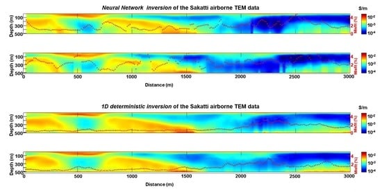
3.2. Field Example
4. Discussion
- It can allow the optimization of the survey design while the acquisition of the ATEM is on-going. In fact, the development of an effective training dataset and the associate ANN can be performed before the survey—or it can be even based on the outcomes from the first flight(s) of the survey if the area is assumed to be relatively “stationary”—and, once the ANN is available, reliable results can be almost instantaneously obtained just after each flight. In turn, this can lead to real-time rearrangements of the original tentative survey plans in order to maximize the VoI (Value of Information) of the measurements to be further collected [57].
- The ANN speed can be extremely useful for effective Quality Check (QC) of the data during the survey.
- The availability of a good starting model (derived from the ANN inversion) can be used to speed-up the 1D deterministic inversion by reducing the number of iterations.
5. Conclusions
Author Contributions
Funding
Acknowledgments
Conflicts of Interest
References
- Zhdanov, M.S.; Alfouzan, F.A.; Cox, L.; Alotaibi, A.; Alyousif, M.; Sunwall, D.; Endo, M. Large-scale 3D modeling and inversion of multiphysics airborne geophysical data: A case study from the Arabian Shield, Saudi Arabia. Minerals 2018, 8, 271. [Google Scholar] [CrossRef]
- Witherly, K. The quest for the Holy Grail in mining geophysics: A review of the development and application of airborne EM systems over the last 50 years. Lead. Edge 2000, 19, 270–274. [Google Scholar] [CrossRef]
- Alfouzan, F.A.; Alotaibi, A.M.; Cox, L.H.; Zhdanov, M.S. Spectral Induced Polarization Survey with Distributed Array System for Mineral Exploration: Case Study in Saudi Arabia. Minerals 2020, 10, 769. [Google Scholar] [CrossRef]
- Cudahy, T. Mineral mapping for exploration: An Australian journey of evolving spectral sensing technologies and industry collaboration. Geosciences 2016, 6, 52. [Google Scholar] [CrossRef]
- Fountain, D. Airborne electromagnetic systems-50 years of development. Explor. Geophys. 1998, 29, 1–11. [Google Scholar] [CrossRef]
- Fraser, D.C. Resistivity mapping with an airborne multicoil electromagnetic system. Geophysics 1978, 43, 144–172. [Google Scholar] [CrossRef]
- Smith, R.S.; Fountain, D.; Allard, M. The MEGATEM fixed-wing transient EM system applied to mineral exploration: A discovery case history. First Break 2003, 21, 73–77. [Google Scholar]
- Rasmussen, S.; Nyboe, N.S.; Mai, S.; Larsen, J.J. Extraction and use of noise models from transient electromagnetic data. Geophysics 2018, 83, E37–E46. [Google Scholar] [CrossRef]
- Smith, R.S.; Lee, T.J. The moments of the impulse response: A new paradigm for the interpretation of transient electromagnetic data. Geophysics 2002, 67, 1095–1103. [Google Scholar] [CrossRef]
- Annan, A.P.; Lookwood, R. An application of airborne GEOTEM in Australian conditions. Explor. Geophys. 1991, 22, 5–12. [Google Scholar] [CrossRef]
- Chen, T.; Hodges, G.; Miles, P. MULTIPULSE–high resolution and high power in one TDEM system. Explor. Geophys. 2015, 46, 49–57. [Google Scholar] [CrossRef]
- Macnae, J. Improving the accuracy of shallow depth determinations in AEM sounding. Explor. Geophys. 2004, 35, 203–207. [Google Scholar] [CrossRef]
- Peters, G.; Street, G.; Kahimise, I.; Hutchins, D. Regional TEMPEST survey in north-east Namibia. Explor. Geophys. 2015, 46, 27–35. [Google Scholar] [CrossRef]
- Sørensen, K.I.; Auken, E. SkyTEM-A new high-resolution helicopter transient electromagnetic system. Explor. Geophys. 2004, 35, 191–199. [Google Scholar] [CrossRef]
- Leggatt, P.B.; Klinkert, P.S.; Hage, T.B. The Spectrem airborne electromagnetic system—Further developments. Geophysics 2000, 65, 1976–1982. [Google Scholar] [CrossRef]
- Legault, J.M.; Izarra, C.; Prikhodko, A.; Zhao, S.; Saadawi, E.M. Helicopter EM (ZTEM–VTEM) survey results over the Nuqrah copper–lead–zinc–gold SEDEX massive sulphide deposit in the Western Arabian Shield, Kingdom of Saudi Arabia. Explor. Geophys. 2015, 46, 36–48. [Google Scholar] [CrossRef]
- Kwan, K.; Prikhodko, A.; Legault, J.M.; Plastow, G.C.; Kapetas, J.; Druecker, M. VTEM airborne EM, aeromagnetic and gamma-ray spectrometric data over the Cerro Quema high sulphidation epithermal gold deposits, Panama. Explor. Geophys. 2016, 47, 179–190. [Google Scholar] [CrossRef]
- Karshakov, E.V.; Podmogov, Y.G.; Kertsman, V.M.; Moilanen, J. Combined Frequency Domain and Time Domain Airborne Data for Environmental and Engineering Challenges. J. Environ. Eng. Geophys. 2017, 22, 1–11. [Google Scholar] [CrossRef]
- Boyko, W.; Paterson, N.R.; Kwan, K. AeroTEM characteristics and field results. Lead. Edge 2001, 20, 1130–1138. [Google Scholar] [CrossRef]
- Jørgensen, F.; Møller, R.R.; Nebel, L.; Jensen, N.P.; Christiansen, A.V.; Sandersen, P.B. A method for cognitive 3D geological voxel modelling of AEM data. Bull. Eng. Geol. Environ. 2013, 72, 421–432. [Google Scholar] [CrossRef]
- Siemon, B.; Ibs-von Seht, M.; Frank, S. Airborne electromagnetic and radiometric peat thickness mapping of a bog in Northwest Germany (Ahlen-Falkenberger Moor). Remote Sens. 2020, 12, 203. [Google Scholar] [CrossRef]
- Høyer, A.S.; Jørgensen, F.; Sandersen, P.B.E.; Viezzoli, A.; Møller, I. 3D geological modelling of a complex buried-valley network delineated from borehole and AEM data. J. Appl. Geophys. 2015, 122, 94–102. [Google Scholar] [CrossRef]
- Siemon, B.; Christiansen, A.V.; Auken, E. A review of helicopter-borne electromagnetic methods for groundwater exploration. Near Surf. Geophys. 2009, 7, 629–646. [Google Scholar] [CrossRef]
- Sapia, V.; Viezzoli, A.; Jørgensen, F.; Oldenborger, G.A.; Marchetti, M. The impact on geological and hydrogeological mapping results of moving from ground to airborne TEM. J. Environ. Eng. Geophys. 2014, 19, 53–66. [Google Scholar] [CrossRef][Green Version]
- Reninger, P.A.; Martelet, G.; Perrin, J.; Dumont, M. Processing methodology for regional AEM surveys and local implications. Explor. Geophys. 2020, 51, 143–154. [Google Scholar] [CrossRef]
- Liu, R.; Guo, R.; Liu, J.; Liu, Z. An Efficient Footprint-Guided Compact Finite Element Algorithm for 3-D Airborne Electromagnetic Modeling. IEEE Geosci. Remote Sens. Lett. 2019, 16, 1809–1813. [Google Scholar] [CrossRef]
- Auken, E.; Christiansen, A.V. Layered and laterally constrained 2D inversion of resistivity data. Geophysics 2004, 69, 752–761. [Google Scholar] [CrossRef]
- Vignoli, G.; Fiandaca, G.; Christiansen, A.V.; Kirkegaard, C.; Auken, E. Sharp spatially constrained inversion with applications to transient electromagnetic data. Geophys. Prospect. 2014, 63, 243–255. [Google Scholar] [CrossRef]
- Ley-Cooper, A.Y.; Viezzoli, A.; Guillemoteau, J.; Vignoli, G.; Macnae, J.; Cox, L.; Munday, T. Airborne electromagnetic modelling options and their consequences in target definition. Explor. Geophys. 2015, 46, 74–84. [Google Scholar] [CrossRef]
- Viezzoli, A.; Auken, E.; Munday, T. Spatially constrained inversion for quasi 3D modelling of airborne electromagnetic data–an application for environmental assessment in the Lower Murray Region of South Australia. Explor. Geophys. 2009, 40, 173–183. [Google Scholar] [CrossRef]
- Cox, L.H.; Wilson, G.A.; Zhdanov, M.S. 3D inversion of airborne electromagnetic data. Geophysics 2012, 77, WB59–WB69. [Google Scholar] [CrossRef]
- Wolfgram, P.; Karlik, G. Conductivity-depth transform of GEOTEM data. Explor. Geophys. 1995, 26, 179–185. [Google Scholar] [CrossRef]
- Macnae, J.; King, A.; Stolz, N.; Osmakoff, A.; Blaha, A. Fast AEM data processing and inversion. Explor. Geophys. 1998, 29, 163–169. [Google Scholar] [CrossRef]
- Huang, H.; Rudd, J. Conductivity-depth imaging of helicopter-borne TEM data based on a pseudolayer half-space model. Geophysics 2008, 73, F115–F120. [Google Scholar] [CrossRef]
- Dzikunoo, E.A.; Vignoli, G.; Jørgensen, F.; Yidana, S.M.; Banoeng-Yakubo, B. New regional stratigraphic insights from a 3D geological model of the Nasia sub-basin, Ghana, developed for hydrogeological purposes and based on reprocessed B-field data originally collected for mineral exploration. Solid Earth 2020, 11, 349–361. [Google Scholar] [CrossRef]
- Brykov, M.N.; Petryshynets, I.; Pruncu, C.I.; Efremenko, V.G.; Pimenov, D.Y.; Giasin, K.; Sylenko, S.A.; Wojciechowski, S. Machine learning modelling and feature engineering in seismology experiment. Sensors 2020, 20, 4228. [Google Scholar] [CrossRef] [PubMed]
- Núñez-Nieto, X.; Solla, M.; Gómez-Pérez, P.; Lorenzo, H. GPR signal characterization for automated landmine and UXO detection based on machine learning techniques. Remote Sens. 2014, 6, 9729–9748. [Google Scholar] [CrossRef]
- Rymarczyk, T.; Kłosowski, G.; Kozłowski, E. A non-destructive system based on electrical tomography and machine learning to analyze the moisture of buildings. Sensors 2018, 18, 2285. [Google Scholar] [CrossRef]
- Yuan, S.; Liu, J.; Wang, S.; Wang, T.; Shi, P. Seismic waveform classification and first-break picking using convolution neural networks. IEEE Geosci. Remote Sens. Lett. 2018, 15, 272–276. [Google Scholar] [CrossRef]
- Van der Baan, M.; Jutten, C. Neural networks in geophysical applications. Geophysics 2000, 65, 1032–1047. [Google Scholar] [CrossRef]
- Andersen, K.K.; Kirkegaard, C.; Foged, N.; Christiansen, A.V.; Auken, E. Artificial neural networks for removal of couplings in airborne transient electromagnetic data. Geophys. Prospect. 2016, 64, 741–752. [Google Scholar] [CrossRef]
- Gunnink, J.L.; Bosch, J.H.A.; Siemon, B.; Roth, B.; Auken, E. Combining ground-based and airborne EM through Artificial Neural Networks for modelling glacial till under saline groundwater conditions. Hydrol. Earth Syst. Sci. 2012, 16, 3061. [Google Scholar] [CrossRef]
- Bhuiyan, M.; Sacchi, M. Optimization for sparse acquisition. In SEG Technical Program Expanded Abstracts. In Proceedings of the Society of Exploration Geophysicists 85th Annual Meetings and International Expositions, New Orleans, LA, USA, 18–23 October 2015. [Google Scholar]
- Latiff, A.H.A.; Ghosh, D.P.; Latiff, N.M.A.A. Optimizing acquisition geometry in shallow gas cloud using particle swarm optimization approach. Int. J. Comput. Intell. Syst. 2017, 10, 1198–1210. [Google Scholar] [CrossRef]
- Curtis, A. Optimal design of focused experiments and surveys. Geophys. J. Int. 1999, 139, 205–215. [Google Scholar] [CrossRef]
- Auken, E.; Christiansen, A.V.; Kirkegaard, C.; Fiandaca, G.; Schamper, C.; Behroozmand, A.A.; Binley, A.; Nielsen, E.; Effersø, F.; Christensen, N.B.; et al. An overview of a highly versatile forward and stable inverse algorithm for airborne, ground-based and borehole electromagnetic and electric data. Explor. Geophys. 2015, 46, 223–235. [Google Scholar] [CrossRef]
- Vignoli, G.; Sapia, V.; Menghini, A.; Viezzoli, A. Examples of improved inversion of different airborne electromagnetic datasets via sharp regularization. J. Environ. Eng. Geophys. 2017, 22, 51–61. [Google Scholar] [CrossRef]
- Vignoli, G.; Deiana, R.; Cassiani, G. Focused inversion of vertical radar profile (VRP) traveltime data. Geophysics 2012, 77, H9–H18. [Google Scholar] [CrossRef]
- Vignoli, G.; Guillemoteau, J.; Barreto, J.; Rossi, M. Reconstruction, with tunable sparsity levels, of shear-wave velocity profiles from surface wave data. Geophys. J. Int. under review.
- Bishop, C.M. Pattern Recognition and Machine Learning; Springer: New York, NY, USA, 2006. [Google Scholar]
- Alpaydin, E. Introduction to Machine Learning; MIT Press: Cambridge, MA, USA, 2004. [Google Scholar]
- Han, D.; Lee, J.; Im, J.; Sim, S.; Lee, S.; Han, H. A novel framework of detecting convective initiation combining automated sampling, machine learning, and repeated model tuning from geostationary satellite data. Remote Sens. 2019, 11, 1454. [Google Scholar] [CrossRef]
- Liu, Y.; Starzyk, J.A.; Zhu, Z. Optimized Approximation Algorithm in Neural Networks without Overfitting. IEEE Trans. Neural Netw. 2008, 19, 983–995. [Google Scholar] [PubMed]
- Duda, R.O.; Hart, P.E.; Stork, D.G. Pattern Classification; John Wiley & Sons: New York, NY, USA, 2012. [Google Scholar]
- Brownscombe, W.; Ihlenfeld, C.; Coppard, J.; Hartshorne, C.; Klatt, S.; Siikaluoma, J.K.; Herrington, R.J. The Sakatti Cu-Ni-PGE sulfide deposit in northern Finland. In Mineral Deposits of Finland; Lahtinen, R., O’Brien, H., Maier, W.D., Eds.; Elsevier: Amsterdam, The Netherlands, 2015; pp. 211–252. [Google Scholar]
- Kesselring, M.; Wagner, F.; Kirsch, M.; Ajjabou, L.; Gloaguen, R. Sustainable Test Sites for Mineral Exploration: Development of Sustainable Test Sites and Knowledge Spillover for Industry. Sustainability 2020, 12, 2016. [Google Scholar] [CrossRef]
- Eidsvik, J.; Bhattacharjya, D.; Mukerji, T. Value of information of seismic amplitude and CSEM resistivity. Geophysics 2008, 73, R59–R69. [Google Scholar] [CrossRef]
- Zhang, F.; Chan, P.P.; Biggio, B.; Yeung, D.S.; Roli, F. Adversarial feature selection against evasion attacks. IEEE Trans. Cybern. 2015, 46, 766–777. [Google Scholar] [CrossRef] [PubMed]
- Biggio, B.; Russu, P.; Didaci, L.; Roli, F. Adversarial biometric recognition: A review on biometric system security from the adversarial machine-learning perspective. IEEE Signal Process. Mag. 2015, 32, 31–41. [Google Scholar] [CrossRef]


Publisher’s Note: MDPI stays neutral with regard to jurisdictional claims in published maps and institutional affiliations. |
© 2020 by the authors. Licensee MDPI, Basel, Switzerland. This article is an open access article distributed under the terms and conditions of the Creative Commons Attribution (CC BY) license (http://creativecommons.org/licenses/by/4.0/).
Share and Cite
Bai, P.; Vignoli, G.; Viezzoli, A.; Nevalainen, J.; Vacca, G. (Quasi-)Real-Time Inversion of Airborne Time-Domain Electromagnetic Data via Artificial Neural Network. Remote Sens. 2020, 12, 3440. https://doi.org/10.3390/rs12203440
Bai P, Vignoli G, Viezzoli A, Nevalainen J, Vacca G. (Quasi-)Real-Time Inversion of Airborne Time-Domain Electromagnetic Data via Artificial Neural Network. Remote Sensing. 2020; 12(20):3440. https://doi.org/10.3390/rs12203440
Chicago/Turabian StyleBai, Peng, Giulio Vignoli, Andrea Viezzoli, Jouni Nevalainen, and Giuseppina Vacca. 2020. "(Quasi-)Real-Time Inversion of Airborne Time-Domain Electromagnetic Data via Artificial Neural Network" Remote Sensing 12, no. 20: 3440. https://doi.org/10.3390/rs12203440
APA StyleBai, P., Vignoli, G., Viezzoli, A., Nevalainen, J., & Vacca, G. (2020). (Quasi-)Real-Time Inversion of Airborne Time-Domain Electromagnetic Data via Artificial Neural Network. Remote Sensing, 12(20), 3440. https://doi.org/10.3390/rs12203440