Automatic Extraction and Filtering of OpenStreetMap Data to Generate Training Datasets for Land Use Land Cover Classification


Abstract
1. Introduction
2. Study Areas and Datasets
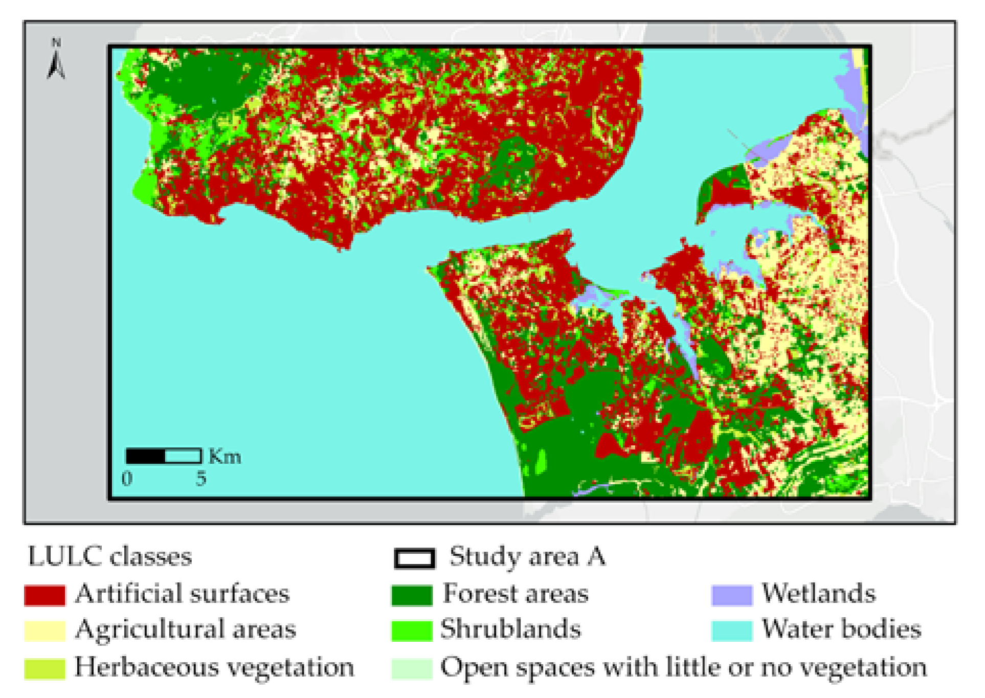
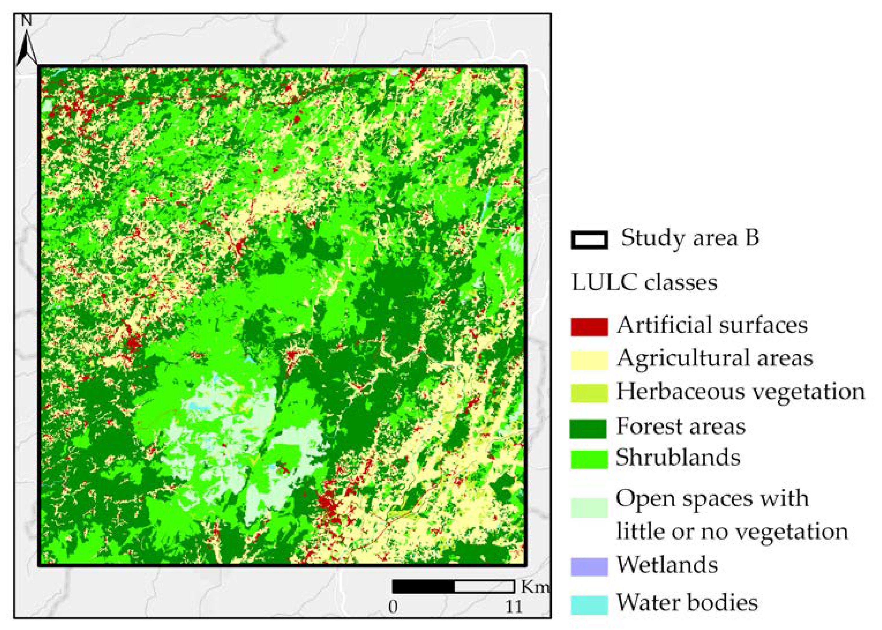
2.1. Study Areas
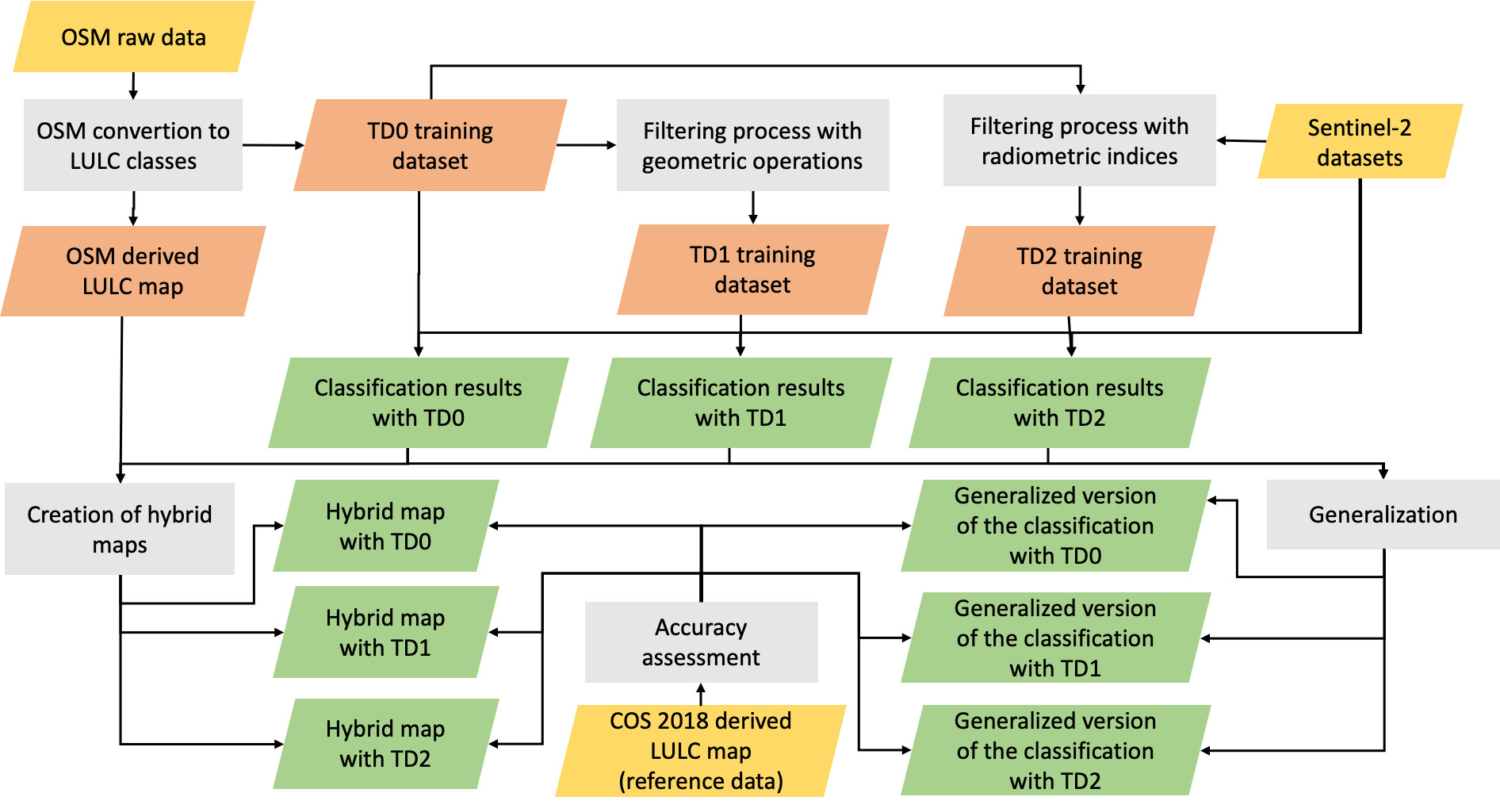
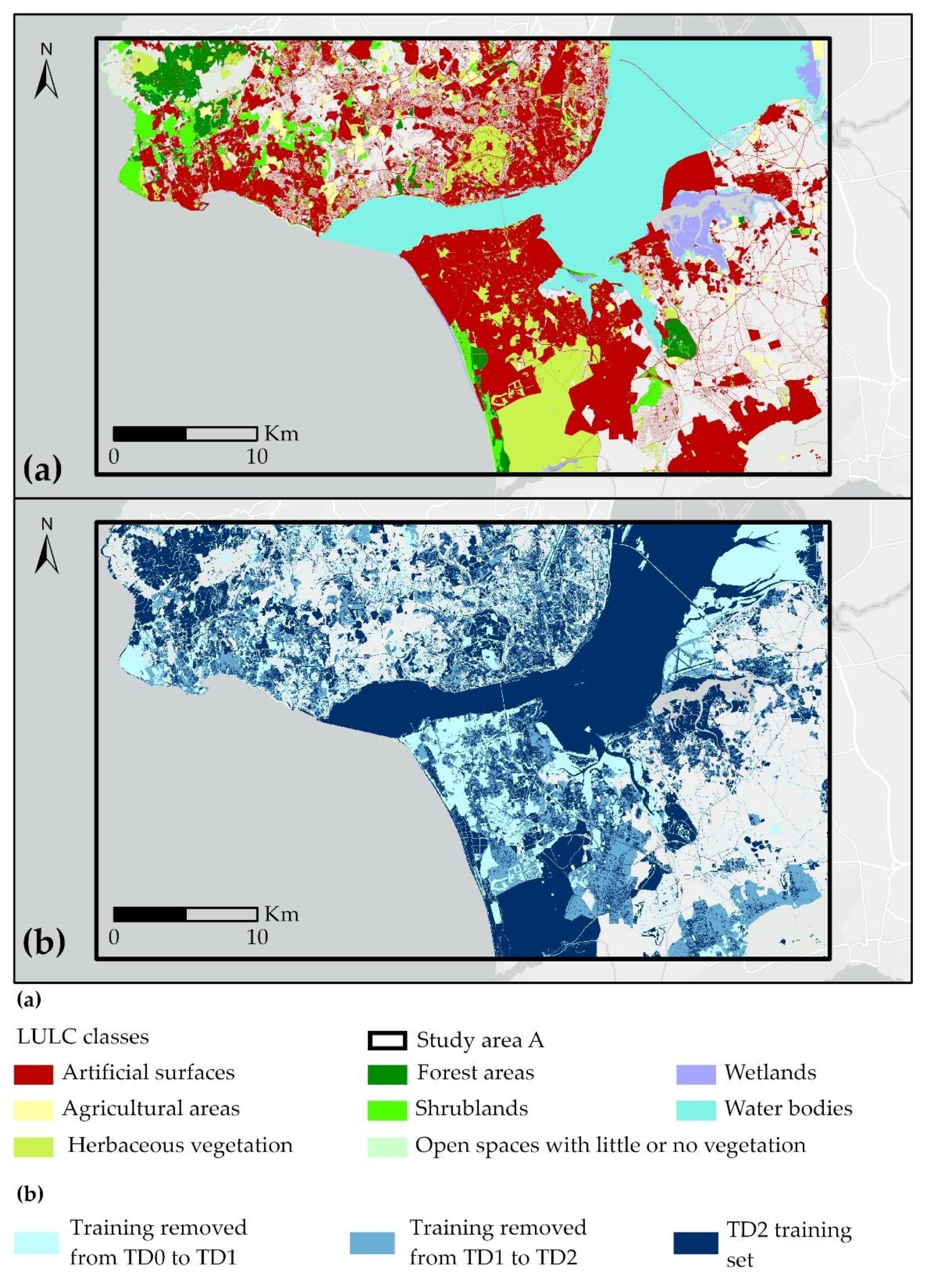
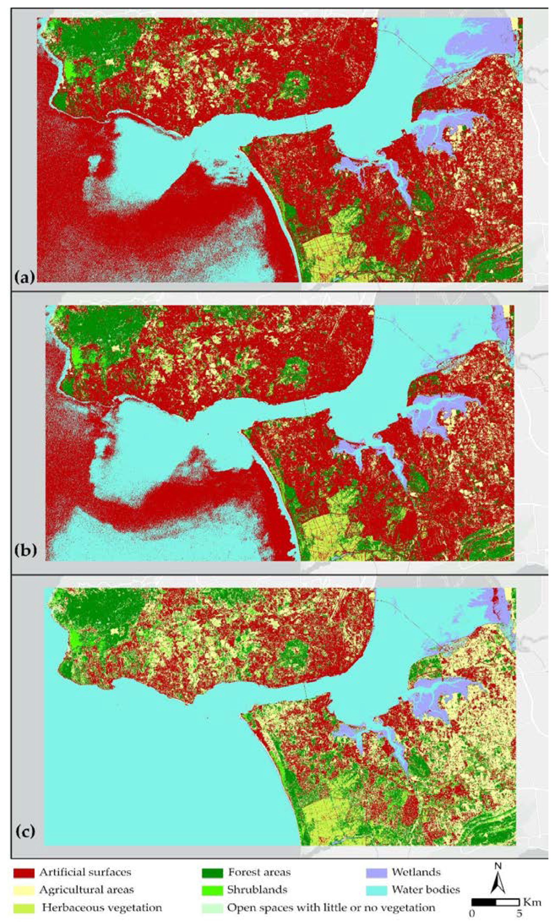
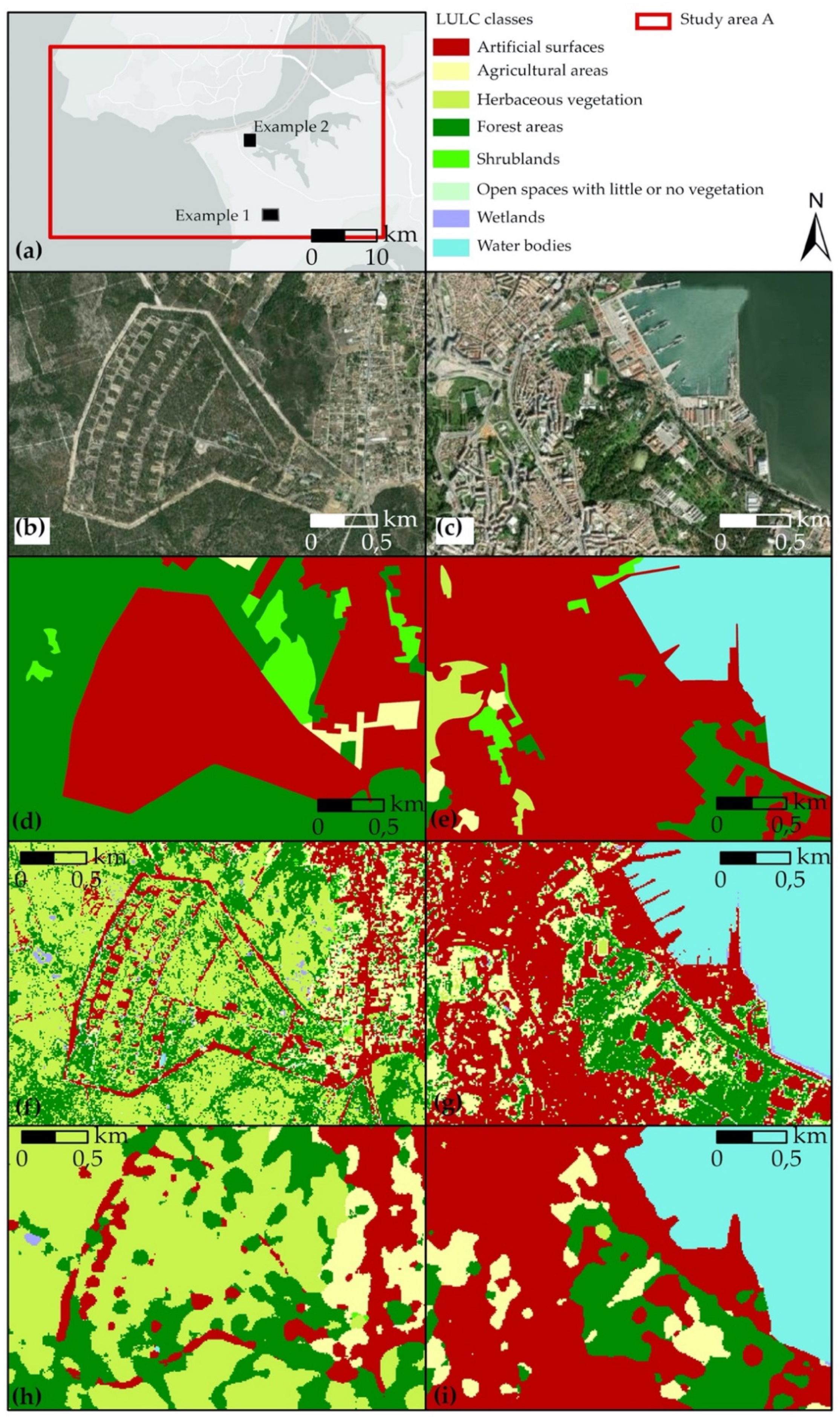
2.1.1. Study Area A
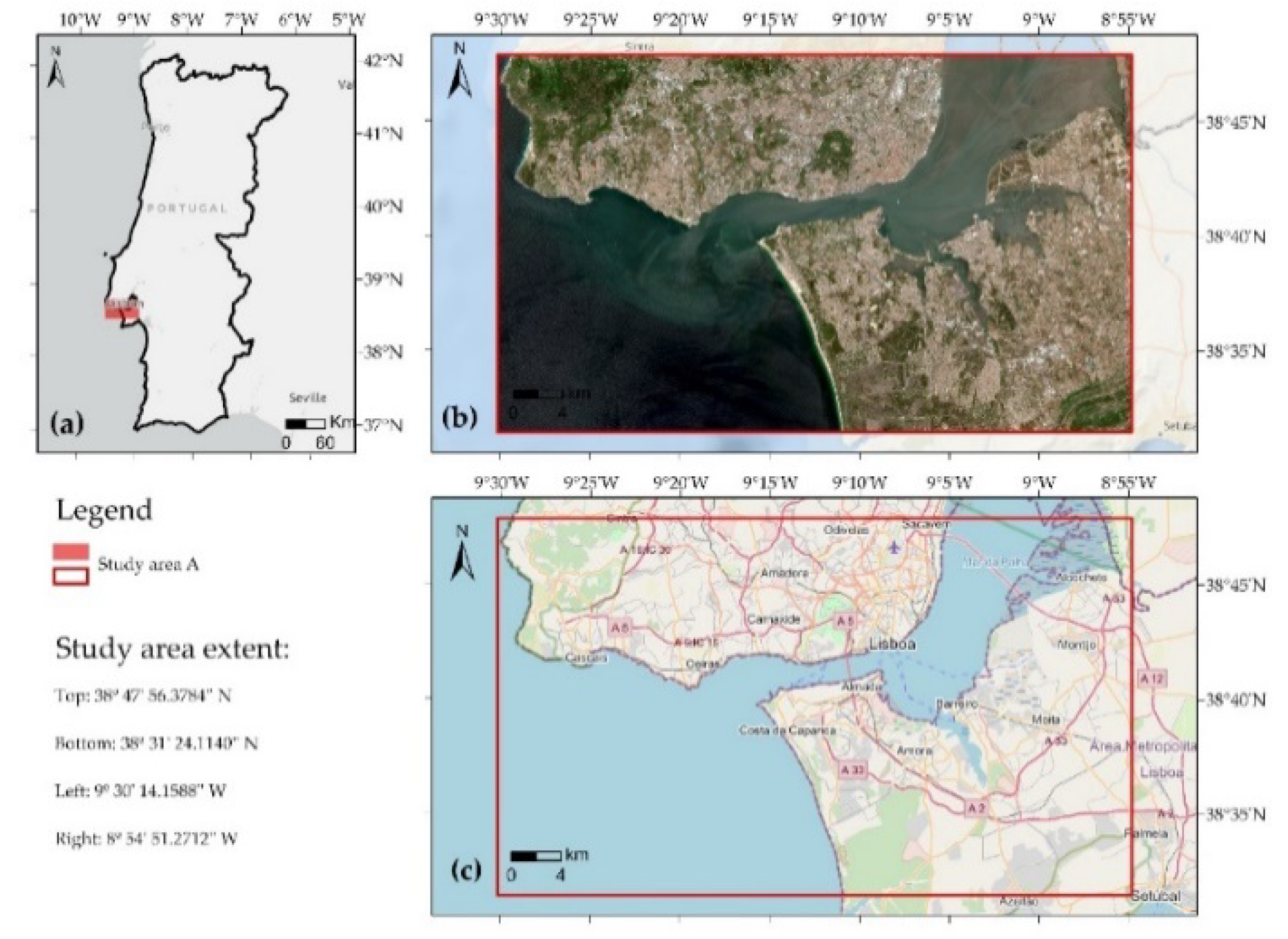
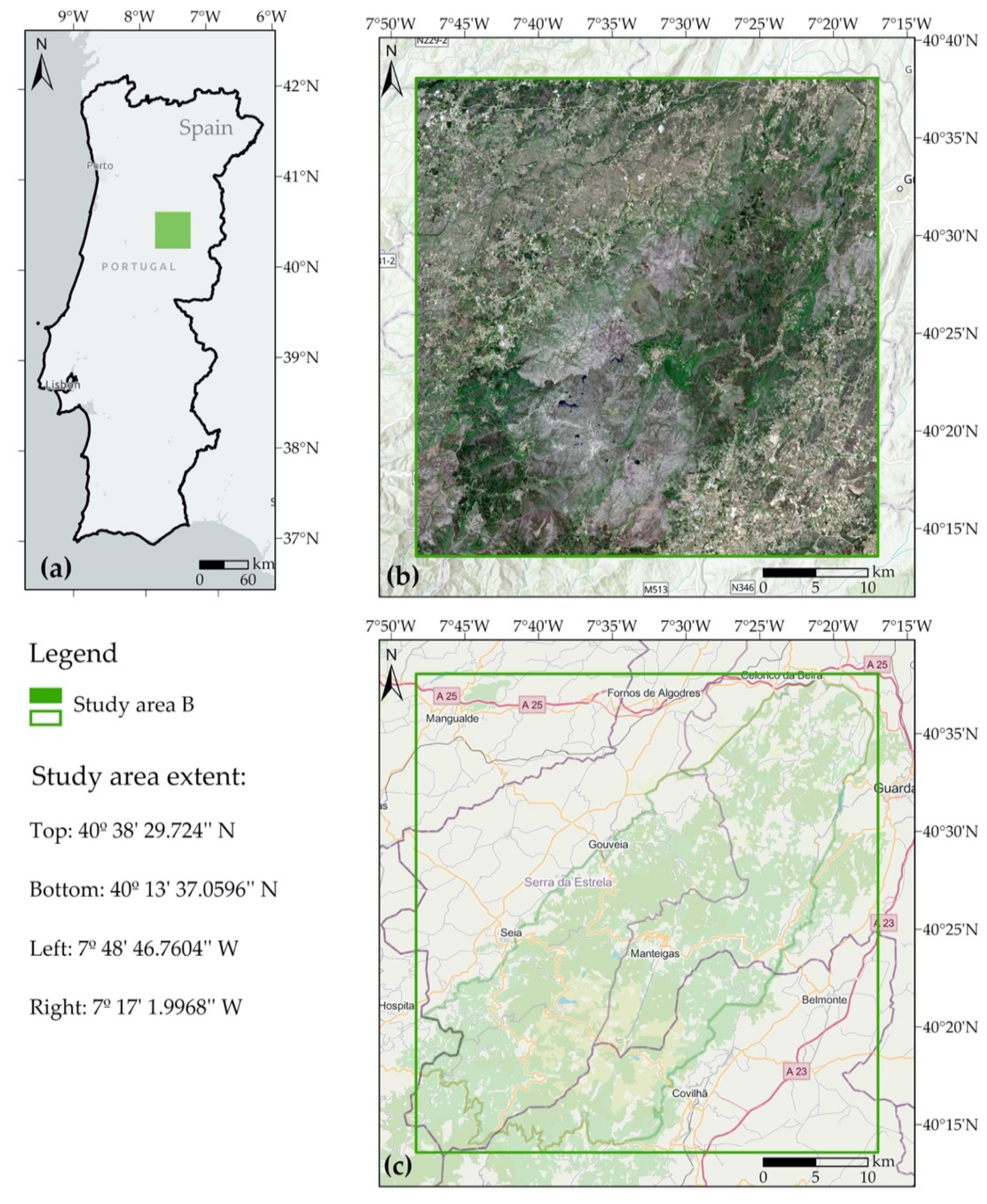
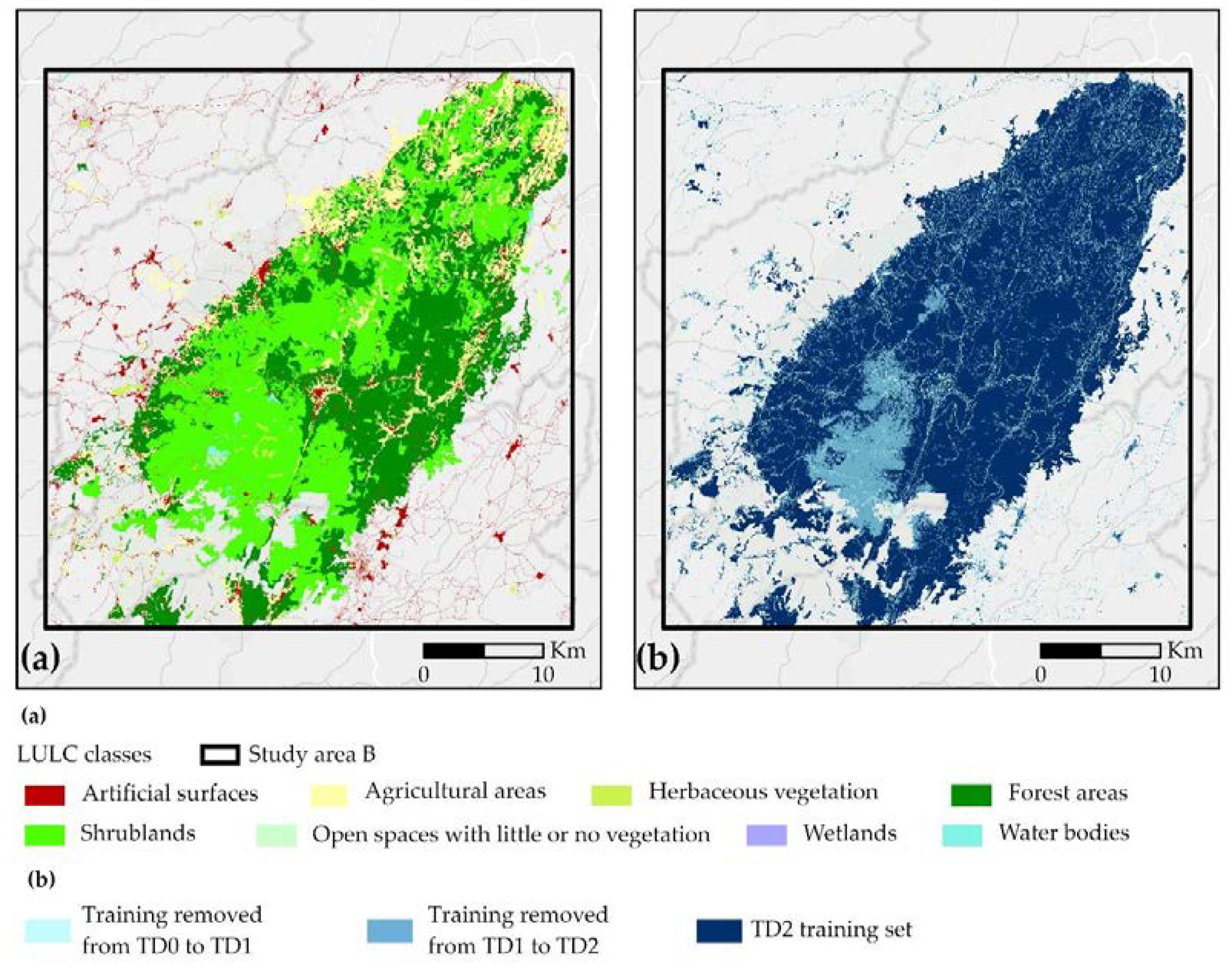
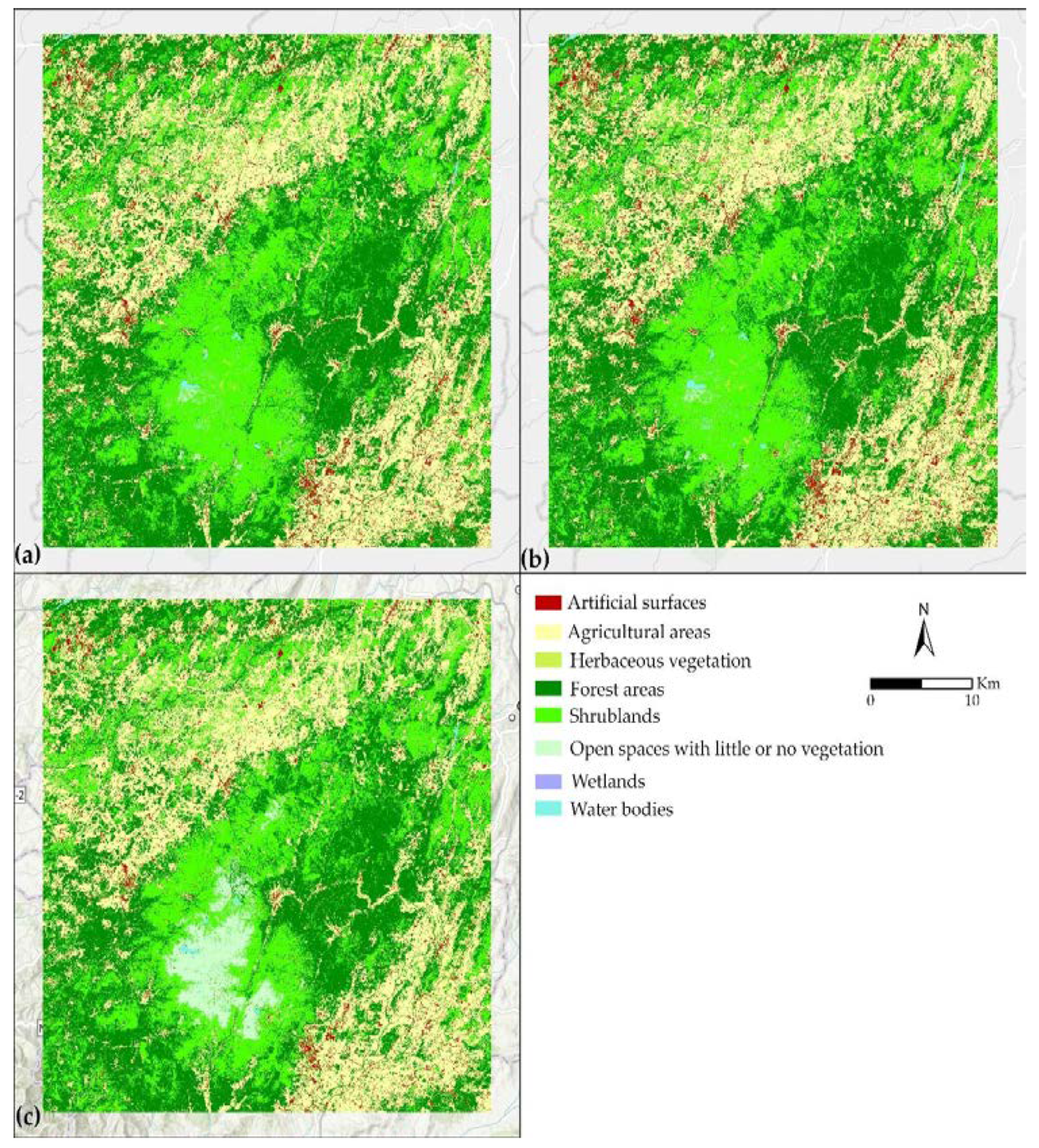
2.1.2. Study Area B
2.2. OpenStreetMap Data
- Nodes—Are points with a geographic location expressed by coordinates (latitude and longitude);
- Ways—Are polylines (if open) or polygons (if closed) and are formed by an ordered list of nodes;
- Relations—Are ordered lists of nodes and ways and are used to express relationships between them, such as a travel root including bus lines and stops;
- Tags—Are associated with nodes, ways or relations and include metadata about them. They are formed by pairs of key-value and are used to describe the properties of the elements, where the key specifies a property which has a value for each element. A list of the tags proposed by the OSM community is available at the OSM Wiki (https://wiki.openstreetmap.org/wiki/Map_Features), but the volunteers may add new tags. Examples of tags (key = value) are building = commercial or landuse = forest.
2.3. Sentinel-2 Satellite Images
2.4. The Portuguese Land Cover Map (COS)
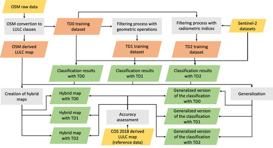
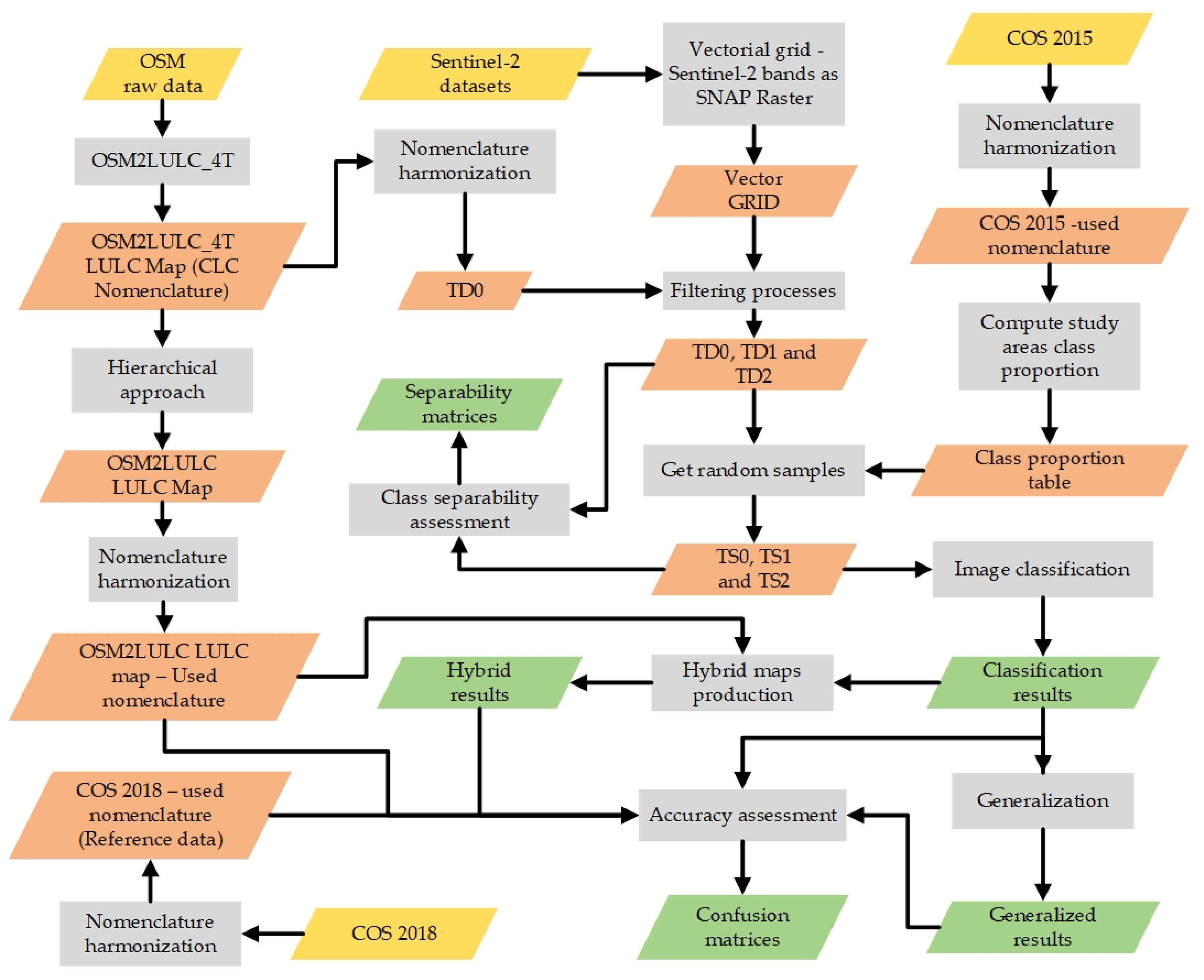
3. Methodology
3.1. Nomenclatures’ Harmonization
3.2. Conversion of OSM Data to LULC
- Mapping the OSM features into the LULC classes of interest;
- converting linear features, such as roads and waterways, into areal features;
- solve inconsistencies resulting from the association of different classes to the same location when there are, for example, overlapping features with different characteristics, or there is missing data indicating that a feature is underground (location = underground).
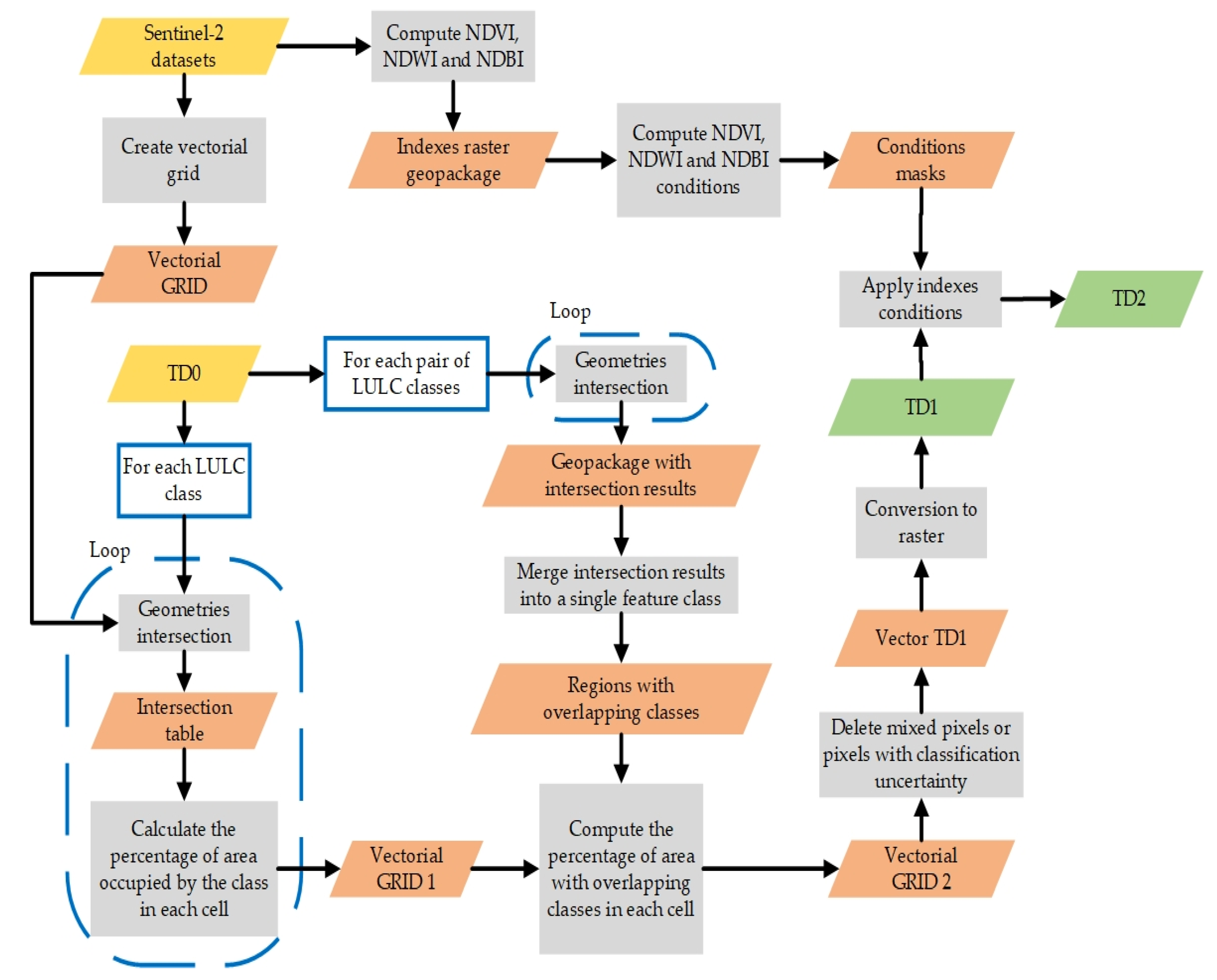
3.3. Training Data
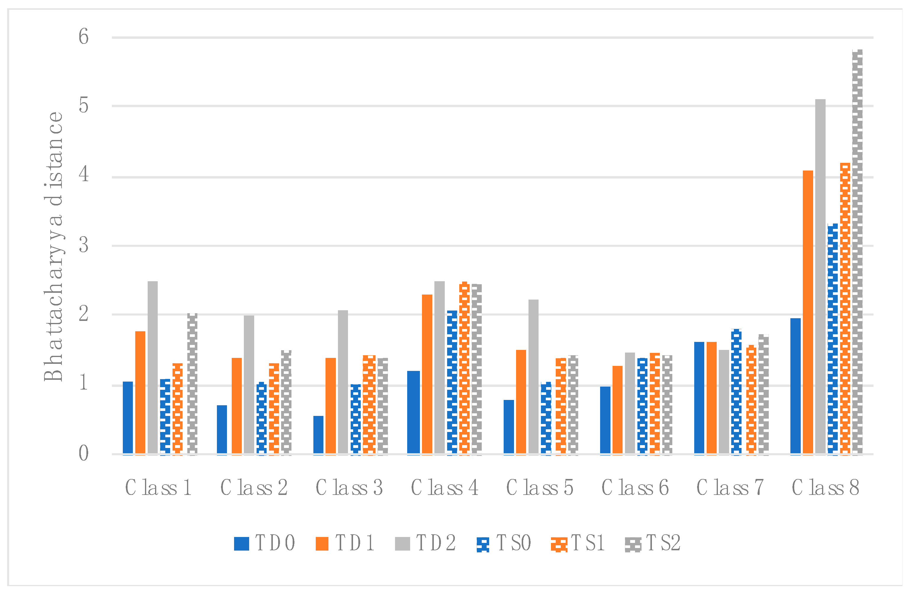
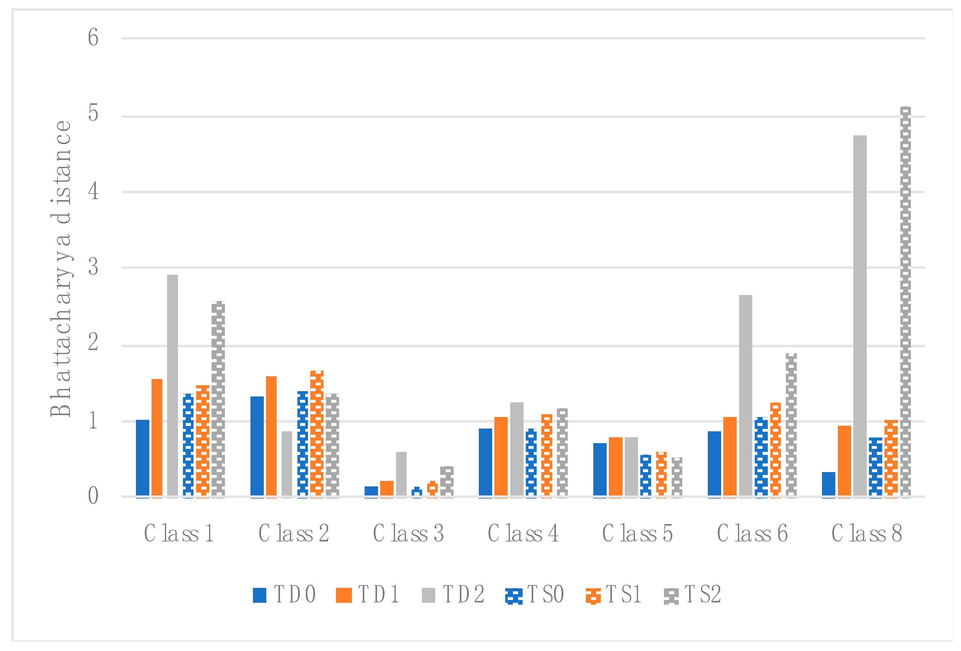
3.4. Classes Separability
3.5. Classification and Generalization
3.6. Accuracy Assessment
3.7. Hybrid Maps
4. Results and Discussion
4.1. Training Data
4.2. Classification and Generalization
4.3. Accuracy Assessment
4.4. Hybrid Maps
5. Conclusions
Author Contributions
Funding
Acknowledgments
Conflicts of Interest
References
- Li, Z.; Liu, S.; Tan, Z.; Sohl, T.L.; Wu, Y. Simulating the effects of management practices on cropland soil organic carbon changes in the Temperate Prairies Ecoregion of the United States from 1980 to 2012. Ecol. Model. 2017, 365, 68–79. [Google Scholar] [CrossRef]
- Ren, W.; Tian, H.; Tao, B.; Yang, J.; Pan, S.; Cai, W.-J.; Lohrenz, S.E.; He, R.; Hopkinson, C.S. Large increase in dissolved inorganic carbon flux from the Mississippi River to Gulf of Mexico due to climatic and anthropogenic changes over the 21st century. J. Geophys. Res. Biogeosci. 2015, 120, 724–736. [Google Scholar] [CrossRef]
- Drake, J.C.; Griffis-Kyle, K.; McIntyre, N.E. Using nested connectivity models to resolve management conflicts of isolated water networks in the Sonoran Desert. Ecosphere 2017, 8, e01652. [Google Scholar] [CrossRef]
- Panlasigui, S.; Davis, A.J.S.; Mangiante, M.J.; Darling, J.A. Assessing threats of non-native species to native freshwater biodiversity: Conservation priorities for the United States. Biol. Conserv. 2018, 224, 199–208. [Google Scholar] [CrossRef]
- Bakillah, M.; Liang, S.; Mobasheri, A.; Jokar Arsanjani, J.; Zipf, A. Fine-resolution population mapping using OpenStreetMap points-of-interest. Int. J. Geogr. Inf. Sci. 2014, 28, 1940–1963. [Google Scholar] [CrossRef]
- Stevens, F.R.; Gaughan, A.E.; Linard, C.; Tatem, A.J. Disaggregating Census Data for Population Mapping Using Random Forests with Remotely-Sensed and Ancillary Data. PLoS ONE 2015, 10, e0107042. [Google Scholar] [CrossRef]
- Schneider, A. Monitoring land cover change in urban and peri-urban areas using dense time stacks of Landsat satellite data and a data mining approach. Remote Sens. Environ. 2012, 124, 689–704. [Google Scholar] [CrossRef]
- European Commission; Directorate-General for Communication. The European Green Deal; European Commission: Brusel, Belgium, 2020; ISBN 978-92-76-17190-4. [Google Scholar]
- Ahiablame, L.; Sinha, T.; Paul, M.; Ji, J.-H.; Rajib, A. Streamflow response to potential land use and climate changes in the James River watershed, Upper Midwest United States. J. Hydrol. Reg. Stud. 2017, 14, 150–166. [Google Scholar] [CrossRef]
- Rajib, A.; Merwade, V. Hydrologic response to future land use change in the Upper Mississippi River Basin by the end of 21st century. Hydrol. Process. 2017, 31, 3645–3661. [Google Scholar] [CrossRef]
- Friedl, M.A.; McIver, D.K.; Hodges, J.C.F.; Zhang, X.Y.; Muchoney, D.; Strahler, A.H.; Woodcock, C.E.; Gopal, S.; Schneider, A.; Cooper, A.; et al. Global land cover mapping from MODIS: Algorithms and early results. Remote Sens. Environ. 2002, 83, 287–302. [Google Scholar] [CrossRef]
- Cihlar, J. Land cover mapping of large areas from satellites: Status and research priorities. Int. J. Remote Sens. 2000, 21, 1093–1114. [Google Scholar] [CrossRef]
- Gislason, P.O.; Benediktsson, J.A.; Sveinsson, J.R. Random Forests for land cover classification. Pattern Recognit. Lett. 2006, 27, 294–300. [Google Scholar] [CrossRef]
- Liu, T.; Abd-Elrahman, A. Multi-view object-based classification of wetland land covers using unmanned aircraft system images. Remote Sens. Environ. 2018, 216, 122–138. [Google Scholar] [CrossRef]
- Pengra, B.W.; Stehman, S.V.; Horton, J.A.; Dockter, D.J.; Schroeder, T.A.; Yang, Z.; Cohen, W.B.; Healey, S.P.; Loveland, T.R. Quality control and assessment of interpreter consistency of annual land cover reference data in an operational national monitoring program. Remote Sens. Environ. 2019, 111261. [Google Scholar] [CrossRef]
- Cavur, M.; Kemec, S.; Nabdel, L.; Duzgun, S. An evaluation of land use land cover (LULC) classification for urban applications with Quickbird and WorldView2 data. In Proceedings of the 2015 Joint Urban Remote Sensing Event, JURSE 2015, Lausanne, Switzerland, 30 March–1 April 2015. [Google Scholar]
- Cao, R.; Zhu, J.; Tu, W.; Li, Q.; Cao, J.; Liu, B.; Zhang, Q.; Qiu, G. Integrating Aerial and Street View Images for Urban Land Use Classification. Remote Sens. 2018, 10, 1553. [Google Scholar] [CrossRef]
- Stehman, S.V. Sampling designs for accuracy assessment of land cover. Int. J. Remote Sens. 2009, 30, 5243–5272. [Google Scholar] [CrossRef]
- Stehman, S.V.; Foody, G.M. Key issues in rigorous accuracy assessment of land cover products. Remote Sens. Environ. 2019, 231, 111199. [Google Scholar] [CrossRef]
- Goodchild, M.F. Citizens as sensors: The world of volunteered geography. GeoJournal 2007, 69, 211–221. [Google Scholar] [CrossRef]
- See, L.; Mooney, P.; Foody, G.; Bastin, L.; Comber, A.; Estima, J.; Fritz, S.; Kerle, N.; Jiang, B.; Laakso, M.; et al. Crowdsourcing, Citizen Science or Volunteered Geographic Information? The Current State of Crowdsourced Geographic Information. ISPRS Int. J. Geo-Inf. 2016, 5, 55. [Google Scholar] [CrossRef]
- OpenStreetMap. Available online: https://www.openstreetmap.org (accessed on 28 August 2020).
- Jokar Arsanjani, J.; Helbich, M.; Bakillah, M.; Hagenauer, J.; Zipf, A. Toward mapping land-use patterns from volunteered geographic information. Int. J. Geogr. Inf. Sci. 2013, 27, 2264–2278. [Google Scholar] [CrossRef]
- Urban Atlas. Available online: https://land.copernicus.eu/local/urban-atlas (accessed on 28 August 2020).
- Patriarca, J.; Fonte, C.C.; Estima, J.; de Almeida, J.-P.; Cardoso, A. Automatic conversion of OSM data into LULC maps: Comparing FOSS4G based approaches towards an enhanced performance. Open Geospat. Data Softw. Stand. 2019, 4, 11. [Google Scholar] [CrossRef]
- Fonte, C.; Minghini, M.; Patriarca, J.; Antoniou, V.; See, L.; Skopeliti, A. Generating Up-to-Date and Detailed Land Use and Land Cover Maps Using OpenStreetMap and GlobeLand30. ISPRS Int. J. Geo-Inf. 2017, 6, 125. [Google Scholar] [CrossRef]
- Fonte, C.C.; Patriarca, J.A.; Minghini, M.; Antoniou, V.; See, L.; Brovelli, M.A. Using OpenStreetMap to Create Land Use and Land Cover Maps: Development of an Application. In Volunteered Geographic Information and the Future of Geospatial Data; IGI Global: Hershey, PA, USA, 2017; p. 25. [Google Scholar]
- Corine Land Cover. Available online: https://land.copernicus.eu/pan-european/corine-land-cover (accessed on 28 August 2020).
- Global Land Cover. Available online: http://www.globallandcover.com (accessed on 28 August 2020).
- Schultz, M.; Voss, J.; Auer, M.; Carter, S.; Zipf, A. Open land cover from OpenStreetMap and remote sensing. Int. J. Appl. Earth Obs. Geoinf. 2017, 63, 206–213. [Google Scholar] [CrossRef]
- Jokar Arsanjani, J.; Helbich, M.; Bakillah, M. Exploiting Volunteered Geographic Information To Ease Land Use Mapping of an Urban Landscape. ISPRS Int. Arch. Photogramm. Remote Sens. Spat. Inf. Sci. 2013, XL-4/W1, 51–55. [Google Scholar] [CrossRef]
- Johnson, B.A.; Iizuka, K. Integrating OpenStreetMap crowdsourced data and Landsat time-series imagery for rapid land use/land cover (LULC) mapping: Case study of the Laguna de Bay area of the Philippines. Appl. Geogr. 2016, 67, 140–149. [Google Scholar] [CrossRef]
- Haufel, G.; Bulatov, D.; Pohl, M.; Lucks, L. Generation of Training Examples Using OSM Data Applied for Remote Sensed Landcover Classification. In Proceedings of the IGARSS 2018 IEEE International Geoscience and Remote Sensing Symposium, Valencia, Spain, 22–27 July 2018; IEEE: Valencia, Spain, 2018; pp. 7263–7266. [Google Scholar]
- Minghini, M.; Frassinelli, F. OpenStreetMap history for intrinsic quality assessment: Is OSM up-to-date? Open Geospat. Data Softw. Stand. 2019, 4, 1–17. [Google Scholar] [CrossRef]
- Fonte, C.C.; Antoniou, V.; Bastin, L.; Estima, J.; Arsanjani, J.J.; Bayas, J.-C.L.; See, L.; Vatseva, R. Assessing VGI Data Quality. Ubiquity Press 2017. [CrossRef]
- Monteiro, E.; Fonte, C.; Lima, J. Analysing the Potential of OpenStreetMap Data to Improve the Accuracy of SRTM 30 DEM on Derived Basin Delineation, Slope, and Drainage Networks. Hydrology 2018, 5, 34. [Google Scholar] [CrossRef]
- Sentinel 2- MSI instrument. Available online: https://earth.esa.int/web/sentinel/technical-guides/sentinel-2-msi/msi-instrument (accessed on 28 August 2020).
- Direção-Geral do Território. Especificações técnicas da Carta de uso e ocupação do solo de Portugal Continental para 1995, 2007, 2010 e 2015; Direção Geral do Território: Lisboa, Portugal, 2018; p. 103. [Google Scholar]
- DGT. Especificações técnicas da Carta de Uso e Ocupação do Solo (COS) de Portugal Continental para 2018 2019; DGT: Lisboa, Portugal, 2019. [Google Scholar]
- Patriarca, J. jasp382/glass: GLASS v0.0.1; Zenodo: Genève, Switzerland, 2020. [Google Scholar]
- Goward, S.N.; Markham, B.; Dye, D.G.; Dulaney, W.; Yang, J. Normalized difference vegetation index measurements from the advanced very high resolution radiometer. Remote Sens. Environ. 1991, 35, 257–277. [Google Scholar] [CrossRef]
- McFeeters, S.K. The use of the Normalized Difference Water Index (NDWI) in the delineation of open water features. Int. J. Remote Sens. 1996, 17, 1425–1432. [Google Scholar] [CrossRef]
- Zha, Y.; Gao, J.; Ni, S. Use of normalized difference built-up index in automatically mapping urban areas from TM imagery. Int. J. Remote Sens. 2003, 24, 583–594. [Google Scholar] [CrossRef]
- Xuan, G.; Zhu, X.; Chai, P.; Zhang, Z.; Shi, Y.; Dongdong, Y. Feature Selection based on the Bhattacharyya Distance. In Proceedings of the 18th International Conference on Pattern Recognition (ICPR’06), Hong Kong, China, 20–24 August 2006; pp. 1232–1235. [Google Scholar]
- McLachlan, G.J. Mahalanobis distance. Resonance 1999, 4, 20–26. [Google Scholar] [CrossRef]
- Cutler, A.; Cutler, D.R.; Stevens, J.R. Random Forests. In Ensemble Machine Learning; Zhang, C., Ma, Y., Eds.; Springer: Boston, MA, USA, 2012; ISBN 978-1-4419-9325-0. [Google Scholar]
- Sklearn. Available online: https://scikit-learn.org/stable/modules/generated/sklearn.ensemble.RandomForestClassifier.html (accessed on 28 August 2020).


| Band | Central Wavelength/Bandwidth | Spatial Resolution |
|---|---|---|
| B1 (Aerosol retrieval) | 443 nm/20 nm | 60 m |
| B2 (Blue) | 490 nm/65 nm | 10 m |
| B3 (Green) | 560 nm/35 nm | 10 m |
| B4 (Red) | 665 nm/30 nm | 10 m |
| B5 (Vegetation red-edge) | 705 nm/15 nm | 20 m |
| B6 (Vegetation red-edge) | 740 nm/15 nm | 20 m |
| B7 (Vegetation red-edge) | 783 nm/20 nm | 20 m |
| B8 (Near-infrared) | 842 nm/115 nm | 10 m |
| B8a (Vegetation red-edge) | 865 nm/20 nm | 20 m |
| B9 (Water vapor retrieval) | 945 nm/20 nm | 60 m |
| B10 (Cirrus cloud detection) | 1380 nm/30 nm | 60 m |
| B11 (SWIR) | 1610 nm/90 nm | 20 m |
| B12 (SWIR) | 2190 nm/180 nm | 20 m |
| Satellite | Product Type | Collection Date | Sentinel GRID | |
|---|---|---|---|---|
| Study area A | Sentinel-2A | Level-2A | 21 March 2018 | T29SMC |
| Sentinel-2A | Level-2A | 19 June 2018 | T29SMC | |
| Sentinel-2B | Level-2A | 22 October 2018 | T29SMC | |
| Study area B | Sentinel-2B | Level-2A | 26 March 2018 | T29TPE |
| Sentinel-2A | Level-2A | 19 June 2018 | T29TPE | |
| Sentinel-2B | Level-2A | 22 October 2018 | T29TPE |
| Class Code | COS 2015 | COS 2018 |
|---|---|---|
| 1 | Artificial surfaces | Artificial surfaces |
| 2 | Agricultural areas | Agriculture |
| 3 | Forest areas and natural spaces | Pasture |
| 4 | Wetlands | Agroforest surfaces |
| 5 | Water bodies | Forests |
| 6 | Shrubs | |
| 7 | Open spaces or with little or no vegetation | |
| 8 | Wetlands | |
| 9 | Superficial water bodies |
| Used Classes | OSM2LULC | COS 2015 | COS 2018 |
|---|---|---|---|
| 1.1 Urban fabric 1.2 Industrial, commercial and transport units 1.3 Mine, dump and construction sites 1.4.2 Sport and leisure facilities (excluding golf courses) | 1. Artificial surfaces, excluding:
| 1. Artificial surfaces, excluding:
|
| 2.1 Arable land 2.2 Permanent crops 2.4 Heterogeneous agricultural areas | 2. Agriculture, excluding:
| 2. Agriculture |
| 1.4.1 Green urban areas 2.3 Pastures 3.2.1 Natural grasslands 1.4.2 Sport and leisure facilities (only golf courses) | 1.4.1.00.0 Public green spaces 1.4.2.01.1 Golf courses 2.3 Permanent pastures 3.2.1 Herbaceous | 3 Herbaceous 1.6.1.1 Golf courses 1.7.1.1 public gardens and playgrounds |
| 3.1 Forests | 2.4.4 Agroforestry 3.1 Forestry | 4 Agroforestry 5 Forestry |
| 3.2.4 Transitional woodland-shrub | 3.2.2 Shrublands | 6 Shrublands |
| 3.3 Open spaces with little or no vegetation | 3.3 Open spaces with little or no vegetation | 7 Open spaces with little or no vegetation |
| 4 Wetlands | 4 Wetlands | 8 Wetlands |
| 5.1 Inland waters 5.2 Marine waters | 5 Water bodies | 9 Water bodies |
| Considered Classes | Study Area A | Study Area B | ||
|---|---|---|---|---|
| Gain (%) | Loss (%) | Gain (%) | Loss (%) | |
| 0.92 | 0.45 | 0.20 | 0.08 |
| 1.04 | 0.92 | 1.15 | 1.34 |
| 0.64 | 1.54 | 0.63 | 0.98 |
| 0.90 | 0.79 | 1.72 | 1.57 |
| 0.92 | 0.65 | 1.77 | 1.55 |
| 0.01 | 0.08 | 0.11 | 0.06 |
| 0.69 | 0.00 | - | - |
| 0.01 | 0.69 | 0.02 | 0.002 |
| Total class change (%) | 5.12 | 5.6 | ||
| Classes | NDVI/Images | NDWI/Images | NDBI/Images |
|---|---|---|---|
| <0.3/all | <0.0/all | >0.0/at least one |
| >0.3/all | <0.0/all | - |
| >0.3/all | <0.0/all | - |
| >0.3/all | <0.0/all | - |
| >0.3/all | <0.0/all | - |
| >0.0/at least one | <0.0/at least one | - |
| >0.0/at least one | <0.0/at least one | - |
| <0.3/at least one | >0.0/all | - |
| Classes | Study Area A | Study Area B | ||||
|---|---|---|---|---|---|---|
| TD0 | TD1 | TD2 | TD0 | TD1 | TD2 | |
| 50.3 | 44.6 | 27.0 | 6.9 | 4.4 | 1.5 |
| 2.7 | 2.7 | 3.6 | 12.8 | 11.9 | 13.4 |
| 9.6 | 11.5 | 15.4 | 2.3 | 2.0 | 2.0 |
| 4.8 | 5.3 | 7.1 | 36.6 | 37.8 | 42.1 |
| 3.7 | 4.4 | 5.9 | 40.4 | 43.1 | 40.5 |
| 0.5 | 0.4 | 0.5 | 0.4 | 0.4 | 0.4 |
| 7.4 | 3.1 | 4.0 | 0.001 | - | - |
| 20.9 | 28.0 | 36.4 | 0.8 | 0.4 | 0.2 |
| Study Area A | Study Area B | |||||
|---|---|---|---|---|---|---|
| Dataset | TD0 | TD1 | TD2 | TD0 | TD1 | TD2 |
| Training datasets | 64 | 74 | 76 | 87 | 89 | 93 |
| Classification results | 55 | 64 | 73 | 65 | 65 | 65 |
| Generalized maps | 55 | 64 | 78 | 69 | 69 | 69 |
| Classification only for regions with OSM data | 69 | 73 | 66 | 66 | 66 | 66 |
| Data obtained with OSM2LULC | 70 | 87 | ||||
| Training Datasets | |||||
|---|---|---|---|---|---|
| Classes | TD0 | TD1 | TD2 | TD1-TD0 | TD2-TD1 |
| 71 | 81 | 97 | 10 | 16 |
| 62 | 72 | 72 | 10 | 0 |
| 12 | 10 | 10 | -3 | 0 |
| 75 | 84 | 84 | 9 | 0 |
| 38 | 40 | 40 | 3 | 0 |
| 42 | 47 | 48 | 5 | 0 |
| 16 | 34 | 34 | 18 | 0 |
| 94 | 97 | 99 | 3 | 1 |
| Classification | |||||
| Classes | TS0 | TS1 | TS2 | TS1-TS0 | TS2-TS1 |
| 41 | 48 | 88 | 7 | 40 |
| 53 | 53 | 42 | 0 | −11 |
| 4 | 5 | 6 | 1 | 1 |
| 72 | 73 | 63 | 1 | −10 |
| 41 | 38 | 26 | −3 | −12 |
| 22 | 25 | 6 | 3 | −19 |
| 15 | 28 | 25 | 13 | −3 |
| 97 | 99 | 99 | 2 | 0 |
| Generalization | |||||
| Classes | TS0 | TS1 | TS2 | TS1-TS0 | TS2-TS1 |
| 41 | 47 | 89 | 6 | 42 |
| 61 | 60 | 45 | −1 | −15 |
| 2 | 4 | 6 | 2 | 2 |
| 75 | 77 | 69 | 2 | −8 |
| 55 | 53 | 42 | −2 | −11 |
| 36 | 45 | 32 | 9 | −13 |
| 16 | 30 | 29 | 14 | −1 |
| 97 | 99 | 99 | 2 | 0 |
| Training Datasets | |||||
| Classes | TD0 | TD1 | TD2 | TD1-TD0 | TD2-TD1 |
| 66 | 97 | 95 | 31 | −2 |
| 73 | 33 | 63 | −40 | 30 |
| 11 | 42 | 59 | 31 | 17 |
| 56 | 24 | 30 | −32 | 6 |
| 21 | 41 | 52 | 20 | 11 |
| 49 | 45 | 48 | −4 | 3 |
| 67 | 61 | 78 | −6 | 17 |
| 85 | 93 | 93 | 8 | 0 |
| Classification | |||||
| Classes | TS0 | TS1 | TS2 | TS1-TS0 | TS2-TS1 |
| 93 | 92 | 62 | −1 | −30 |
| 40 | 40 | 74 | 0 | 34 |
| 3 | 5 | 7 | 2 | 2 |
| 44 | 47 | 58 | 3 | 11 |
| 9 | 14 | 18 | 5 | 4 |
| 46 | 44 | 46 | −2 | 2 |
| 42 | 51 | 60 | 9 | 9 |
| 50 | 68 | 95 | 18 | 27 |
| Generalization | |||||
| Classes | TS0 | TS1 | TS2 | TS1-TS0 | TS2-TS1 |
| 97 | 97 | 75 | 0 | −22 |
| 36 | 36 | 85 | 0 | 49 |
| 2 | 4 | 6 | 2 | 2 |
| 44 | 48 | 64 | 4 | 16 |
| 6 | 9 | 12 | 3 | 3 |
| 47 | 44 | 47 | −3 | 3 |
| 45 | 53 | 66 | 8 | 13 |
| 48 | 67 | 95 | 19 | 28 |
| Training Datasets | |||||
|---|---|---|---|---|---|
| Classes | TD0 | TD1 | TD2 | TD1-TD0 | TD2-TD1 |
| 48 | 68 | 90 | 20 | 22 |
| 99 | 99 | 99 | 0 | 0 |
| 71 | 72 | 69 | 2 | −4 |
| 100 | 100 | 100 | 0 | 0 |
| 80 | 80 | 86 | 0 | 6 |
| 97 | 98 | 98 | 1 | 0 |
| - | - | - | - | - |
| 51 | 93 | 99 | 42 | 6 |
| Classification | |||||
| Classes | TS0 | TS1 | TS2 | TS1-TS0 | TS2-TS1 |
| 52 | 48 | 58 | −4 | 9 |
| 63 | 63 | 63 | 1 | 0 |
| 46 | 47 | 42 | 1 | −6 |
| 71 | 72 | 74 | 0 | 2 |
| 60 | 60 | 59 | 0 | −1 |
| 54 | 53 | 41 | −1 | −12 |
| - | - | - | - | - |
| 93 | 63 | 88 | -29 | 24 |
| Generalization | |||||
| Classes | TS0 | TS1 | TS2 | TS1-TS0 | TS2-TS1 |
| 77 | 72 | 77 | −5 | 5 |
| 63 | 64 | 63 | 1 | −1 |
| 74 | 75 | 56 | 1 | −19 |
| 75 | 75 | 78 | 0 | 3 |
| 65 | 65 | 65 | 0 | 0 |
| 78 | 82 | 42 | 4 | −40 |
| - | - | - | - | - |
| 94 | 78 | 90 | −16 | 12 |
| Training Datasets | |||||
|---|---|---|---|---|---|
| Classes | TD0 | TD1 | TD2 | TD1-TD0 | TD2-TD1 |
| 96 | 98 | 96 | 2 | −2 |
| 86 | 93 | 99 | 8 | 6 |
| 89 | 96 | 99 | 7 | 3 |
| 94 | 97 | 98 | 4 | 1 |
| 98 | 99 | 100 | 2 | 0 |
| 4 | 4 | 7 | 0 | 3 |
| - | - | - | - | - |
| 93 | 97 | 97 | 4 | 0 |
| Classification | |||||
| Classes | TS0 | TS1 | TS2 | TS1-TS0 | TS2-TS1 |
| 47 | 53 | 39 | 6 | −14 |
| 85 | 84 | 85 | −1 | 1 |
| 5 | 6 | 4 | 1 | −2 |
| 73 | 73 | 70 | 0 | −3 |
| 54 | 55 | 54 | 1 | 0 |
| 8 | 8 | 38 | 0 | 30 |
| - | - | - | - | - |
| 38 | 64 | 47 | 26 | −17 |
| Generalization | |||||
| Classes | TS0 | TS1 | TS2 | TS1-TS0 | TS2-TS1 |
| 47 | 55 | 37 | 8 | −18 |
| 91 | 90 | 91 | −1 | 1 |
| 2 | 3 | 1 | 1 | −2 |
| 78 | 77 | 74 | −1 | −3 |
| 56 | 57 | 56 | 1 | −1 |
| 4 | 4 | 38 | 0 | 34 |
| - | - | - | - | - |
| 40 | 58 | 47 | 18 | −11 |
| Class/Gen | Hybrid Map (HM) | HM—Class/HM—Gen | |||||||
|---|---|---|---|---|---|---|---|---|---|
| TS0 | TS1 | TS2 | TS0 | TS1 | TS2 | TS0 | TS1 | TS2 | |
| Study area A | 55/55 | 64/64 | 73/78 | 56 | 62 | 76 | 1/1 | −2/−2 | 3/−2 |
| Study area B | 65/69 | 65/69 | 65/69 | 75 | 75 | 74 | 10/10 | 10/10 | 9/9 |
Publisher’s Note: MDPI stays neutral with regard to jurisdictional claims in published maps and institutional affiliations. |
© 2020 by the authors. Licensee MDPI, Basel, Switzerland. This article is an open access article distributed under the terms and conditions of the Creative Commons Attribution (CC BY) license (http://creativecommons.org/licenses/by/4.0/).
Share and Cite
Fonte, C.C.; Patriarca, J.; Jesus, I.; Duarte, D. Automatic Extraction and Filtering of OpenStreetMap Data to Generate Training Datasets for Land Use Land Cover Classification. Remote Sens. 2020, 12, 3428. https://doi.org/10.3390/rs12203428
Fonte CC, Patriarca J, Jesus I, Duarte D. Automatic Extraction and Filtering of OpenStreetMap Data to Generate Training Datasets for Land Use Land Cover Classification. Remote Sensing. 2020; 12(20):3428. https://doi.org/10.3390/rs12203428
Chicago/Turabian StyleFonte, Cidália C., Joaquim Patriarca, Ismael Jesus, and Diogo Duarte. 2020. "Automatic Extraction and Filtering of OpenStreetMap Data to Generate Training Datasets for Land Use Land Cover Classification" Remote Sensing 12, no. 20: 3428. https://doi.org/10.3390/rs12203428
APA StyleFonte, C. C., Patriarca, J., Jesus, I., & Duarte, D. (2020). Automatic Extraction and Filtering of OpenStreetMap Data to Generate Training Datasets for Land Use Land Cover Classification. Remote Sensing, 12(20), 3428. https://doi.org/10.3390/rs12203428