Agricultural Drought Monitoring by MODIS Potential Evapotranspiration Remote Sensing Data Application

 ,
,  , , , and
Abstract

1. Introduction
- (i)
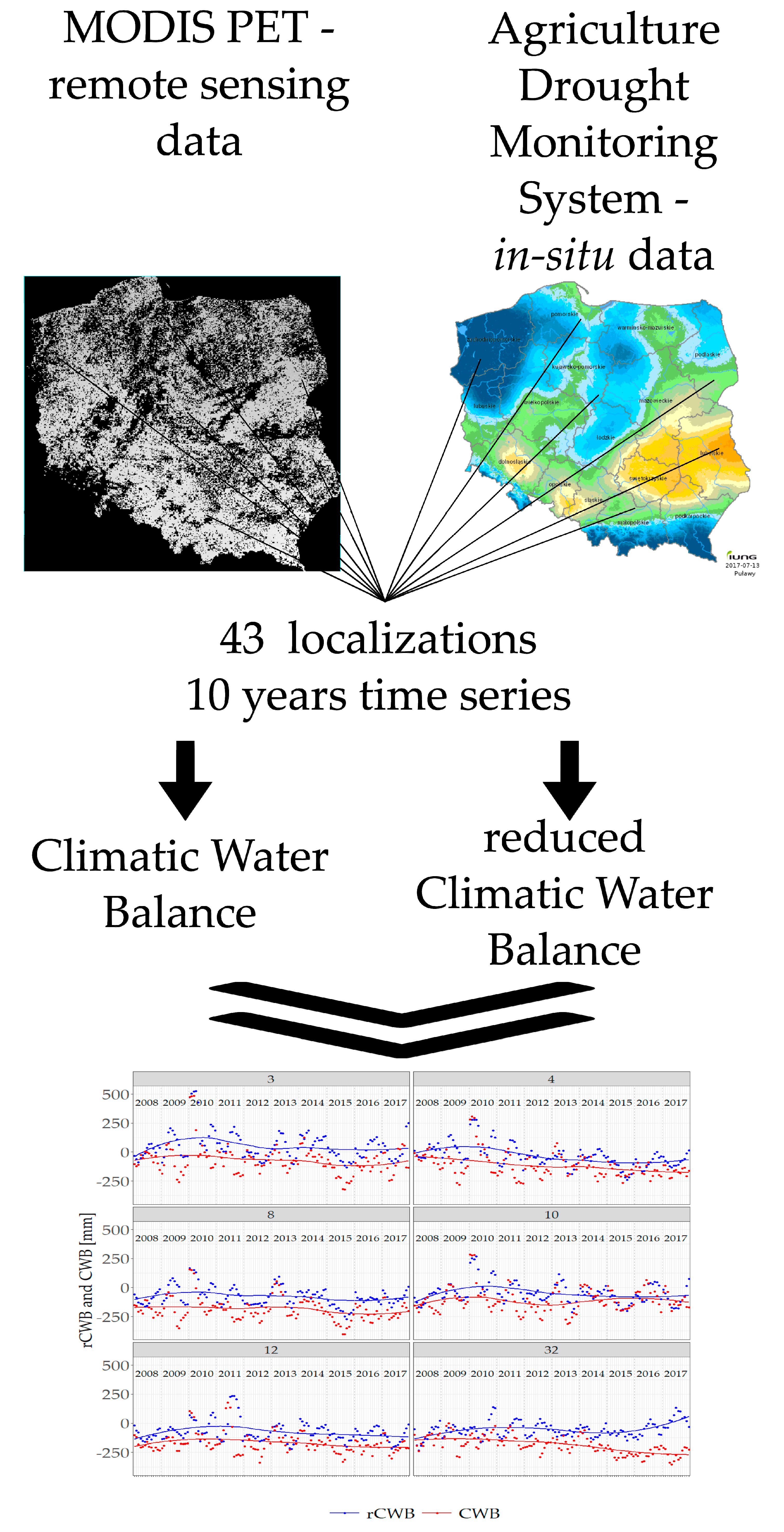
- The currently established in Poland methodology for the rCWB assessment which employed ground-based meteorological station data;
- (ii)
- The CWB obtained using rainfall from ground stations plus remote sensing values of PET from MODIS instrument.
2. Materials and Methods
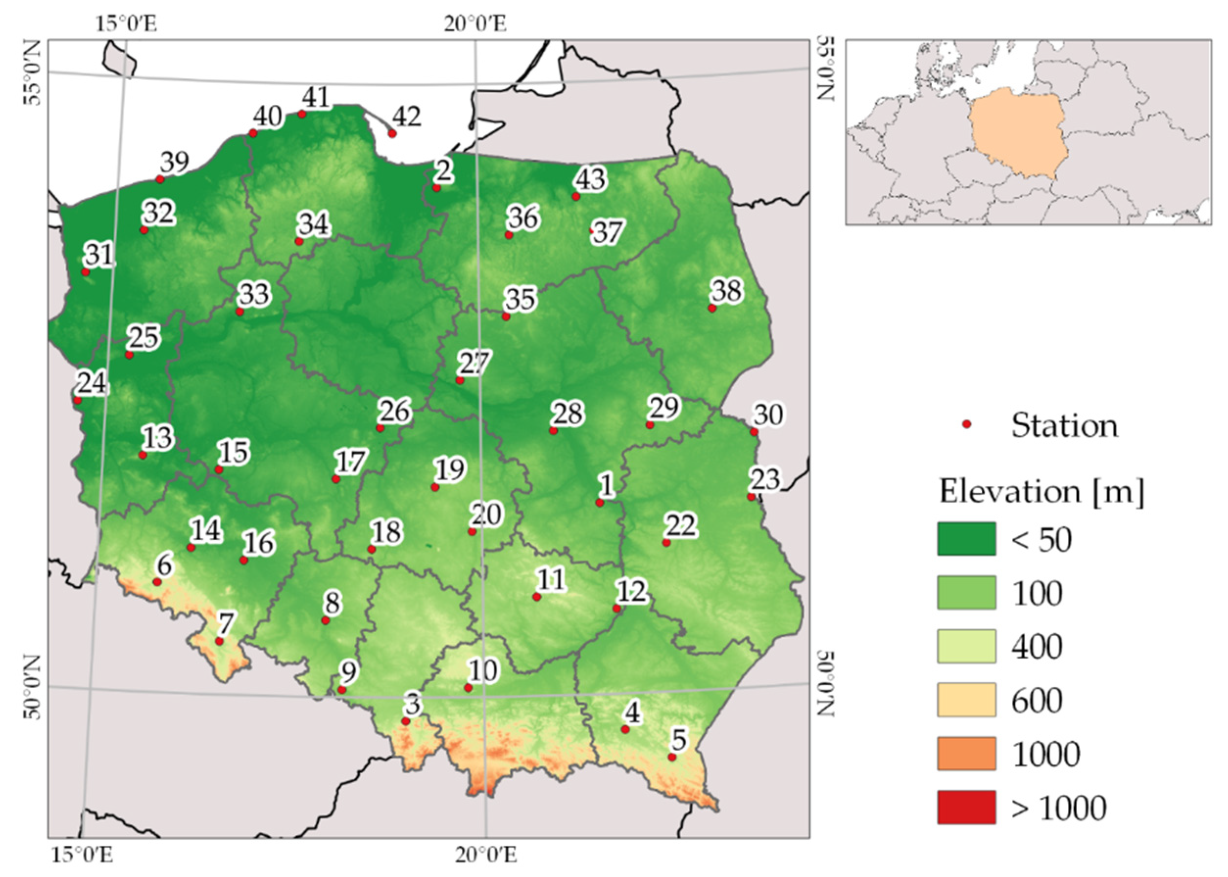
2.1. Input Data, Spatial and Temporal Scale
2.2. Precipitation–P8
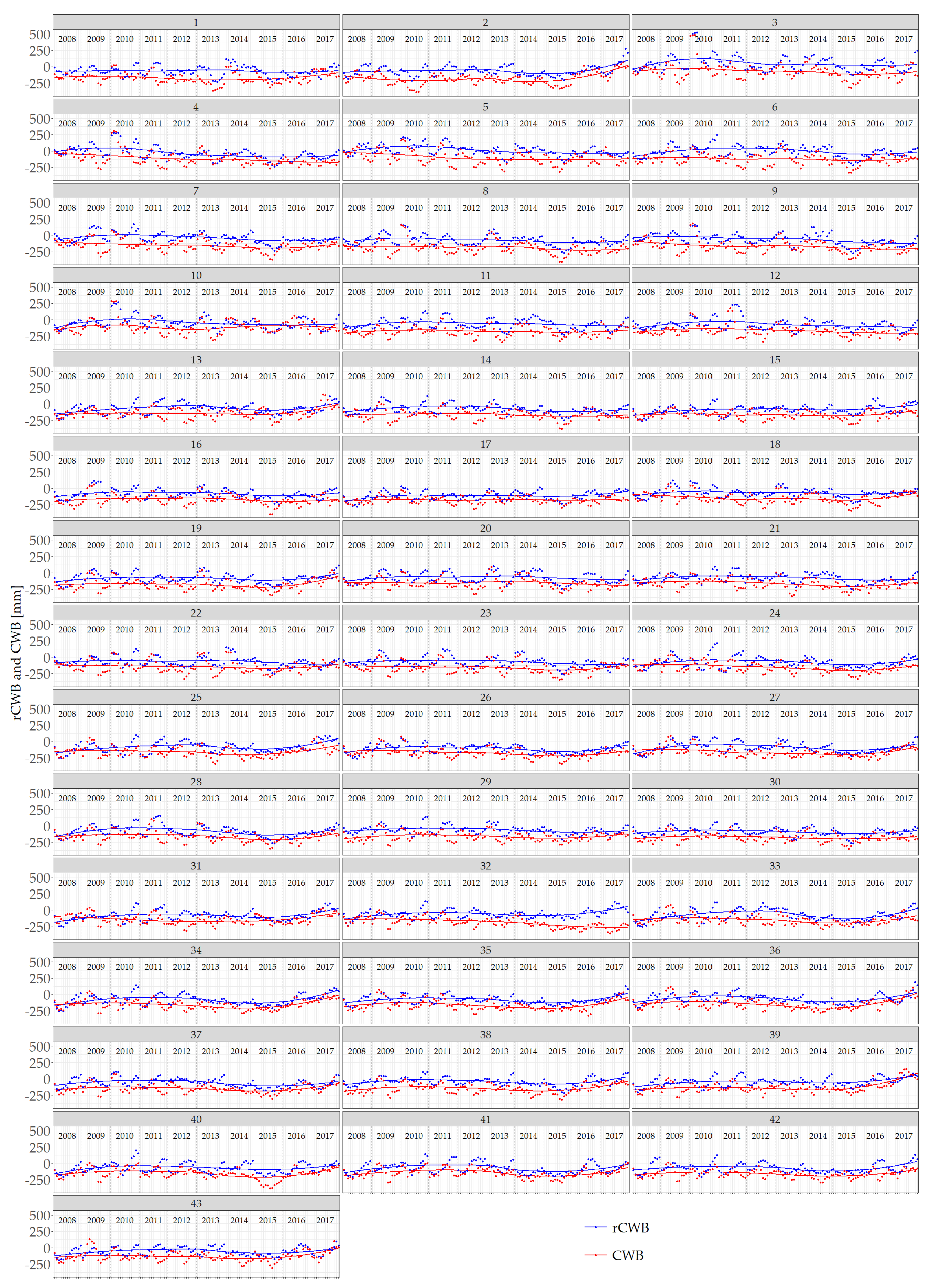
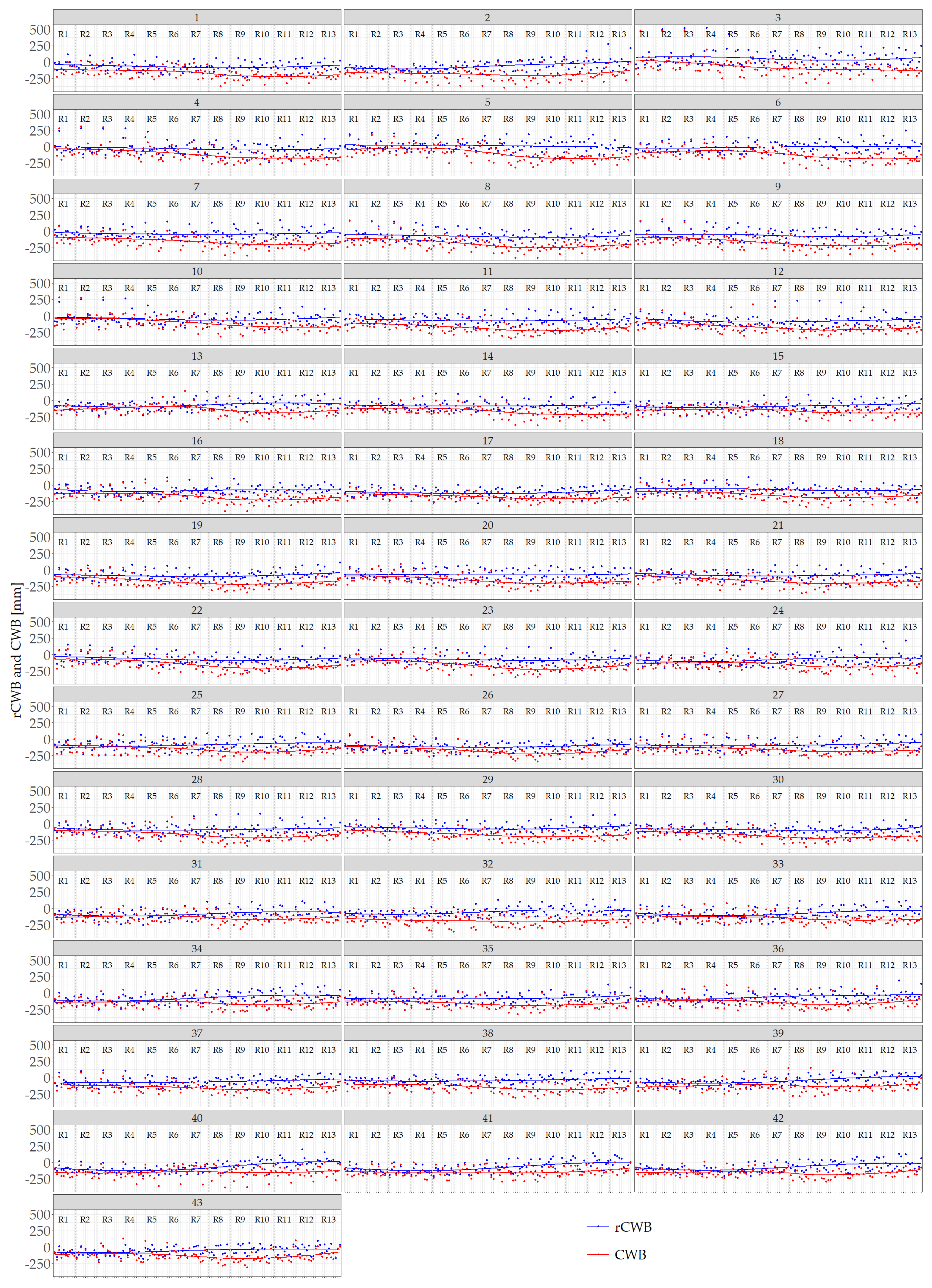
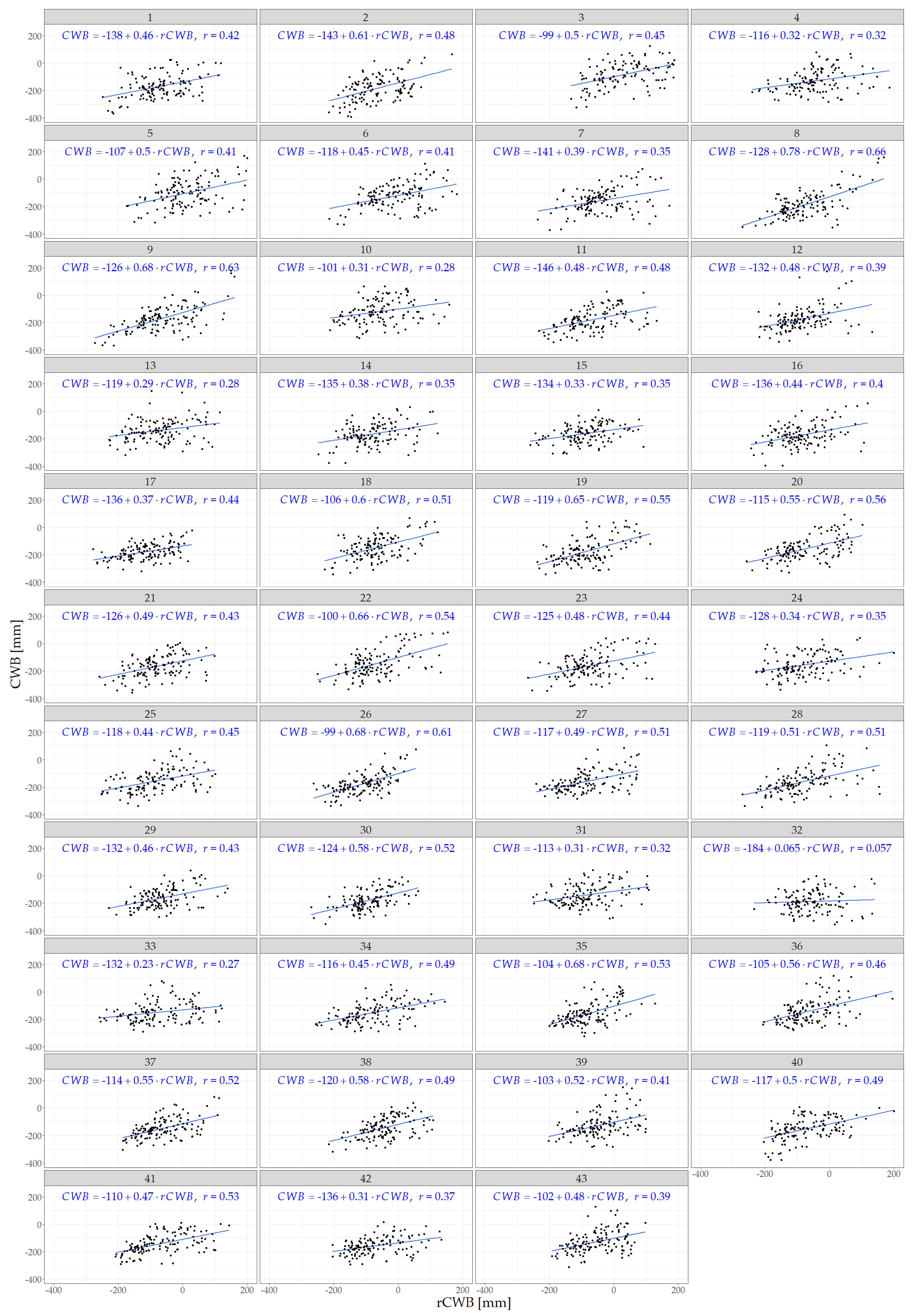
2.3. Reduced Climatic Water Balance—rCWB
2.4. Potential Evapotranspiration from MODIS–PET
2.5. Climatic Water Balance—CWB
2.6. Data Analysis
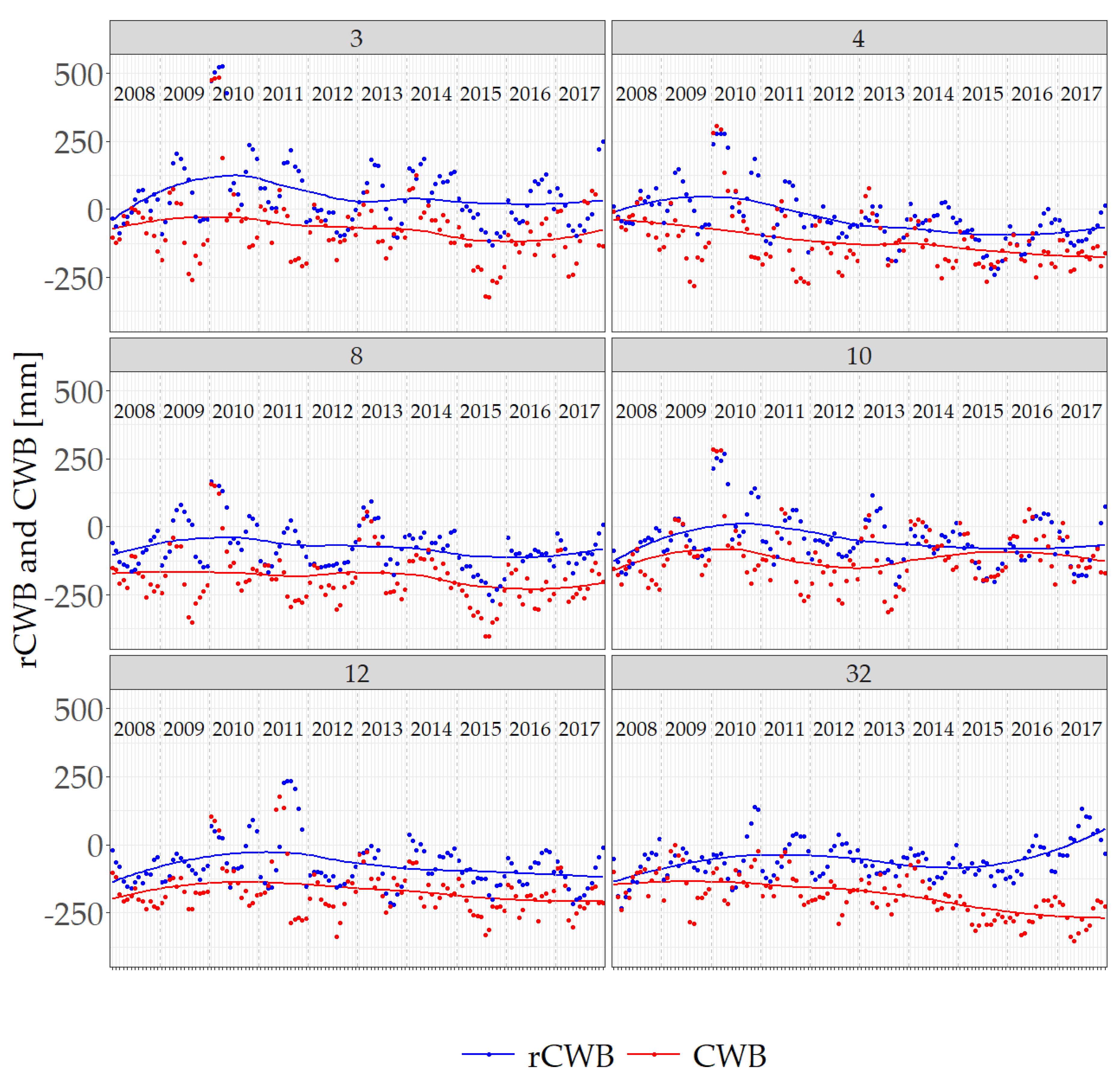
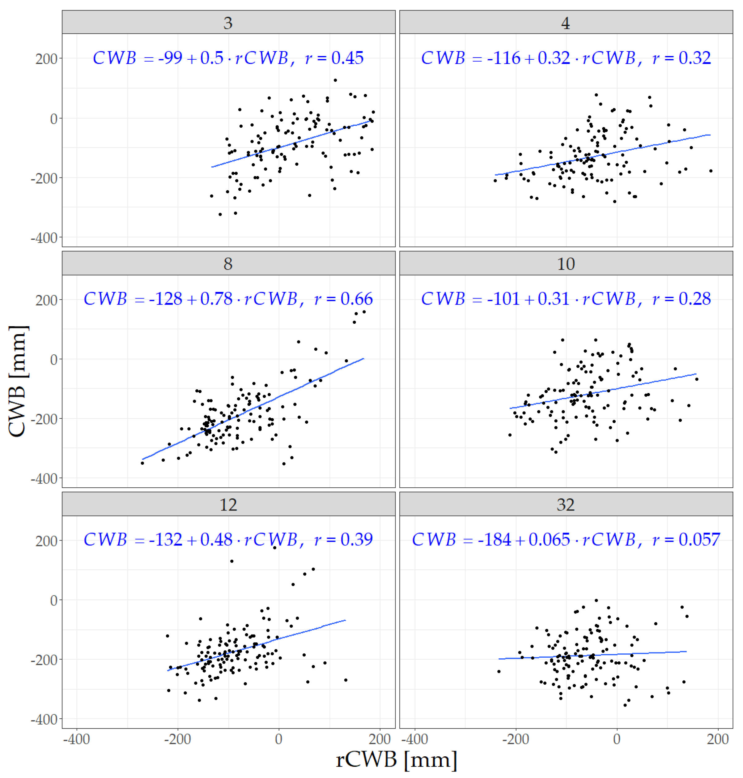
3. Results
4. Discussion
5. Conclusions
Author Contributions
Funding
Acknowledgments
Conflicts of Interest
Appendix A
Appendix B


References
- Gornall, J.; Betts, R.; Burke, E.; Clark, R.; Camp, J.; Willett, K.; Wiltshire, A. Implications of climate change for agricultural productivity in the early twenty-first century. Philos. Trans. R. Soc. B Biol. Sci. 2010, 365, 2973–2989. [Google Scholar] [CrossRef] [PubMed]
- Yu, C.; Huang, X.; Chen, H.; Huang, G.; Ni, S.; Wright, J.S.; Hall, J.; Ciais, P.; Zhang, J.; Xiao, Y.; et al. Assessing the impacts of extreme agricultural droughts in China under climate and socio-economic changes. Earth’s Future 2018, 6, 689–703. [Google Scholar] [CrossRef]
- European Commission. Third Follow up Report to the Communication on Water Scarcity and Droughts in the European Union COM (2007) 414 Final; European Commission: Brussels, Belgium, 2011. [Google Scholar]
- Armenski, T.; Stankov, U.; Dolinaj, D.; Mesaros, M.; Jovanovic, M.; Pantelic, M.; Pavic, D.; Popov, S.; Popovic, L.; Frank, A.; et al. Social and economic impact of drought on stakeholders in agriculture. Geogr. Pannonica 2014, 18, 34–42. [Google Scholar] [CrossRef]
- Borek, D.; Głowacka-Smolis, K.; Gustyn, J.; Kozera, A.; Kozłowska, J.; Lipowska, E.; Marikin, M.; Nowak, T.; Pilaszek, K.; Rybak-Nguyen, E.; et al. Statistical Yearbook of the Republic of Poland; Statistics Poland: Warsaw, Poland, 2018.
- European Commission—EUROSTAT. Available online: https://appsso.eurostat.ec.europa.eu/nui/show.do?dataset=apro_cpsh1&lang=en (accessed on 15 October 2020).
- Somorowska, U. Changes in Drought Conditions in Poland over the Past 60 Years Evaluated by the Standardized Precipitation-Evapotranspiration Index. Acta Geophys. 2016, 64, 2530–2549. [Google Scholar] [CrossRef]
- Svoboda, M.; Fuchs, B. Handbook of Drought Indicators and Indices. World Meteorological Organization (WMO) and Global Water Partnership (GWP). Integrated Drought Management Programme (IDMP). Integrated Drought Management Tools and Guidelines. Series 2. 2016. Available online: https://www.drought.gov/drought/sites/drought.gov.drought/files/GWP_Handbook_of_Drought_Indicators_and_Indices_2016.pdf (accessed on 15 October 2020).
- Allen, R.G.; Pereira, L.S.; Raes, D.; Smith, M. Crop evapotranspiration-Guidelines for computing crop water requirements—FAO Irrigation and drainage. Tech. Rep. 1998, 300, D05109. [Google Scholar]
- Zink, M.; Samaniego, L.; Kumar, R.; Thober, S.; Mai, J.; Schäfer, D.; Marx, A. The German drought monitor. Environ. Res. Lett. 2016, 11, 74002. [Google Scholar] [CrossRef]
- Donald, W. Drought as a Natural Hazard: Concepts and Definitions. Drought, a Global Assessment. 1. 2000. Available online: https://www.researchgate.net/publication/243785200_Drought_as_a_Natural_Hazard_Concepts_and_Definitions (accessed on 15 October 2020).
- Doroszewski, A.; Jadczyszyn, J.; Kozyra, J.; Pudełko, R.; Stuczyński, T.; Mizak, K.; Łopatka, A.; Koza, P.; Górski, T.; Wróblewska, E. Podstawy systemu monitoringu suszy rolniczej. Woda-Środowisko-Obszary Wiejskie 2012, 12, 77–91. [Google Scholar]
- The Government of Republic of Poland. The Act of 7 July 2005 on Insurance of Agricultural Crops and Livestock. J. Law 2005, 150, 1249. [Google Scholar]
- Penman, H.L. Natural evaporation from open water, bare soil and grass. Proc. R. Soc. Lond. Ser. A Math. Phys. Sci. 1948, 193, 120–145. [Google Scholar]
- ADMS. Web-Portal of Agricultural Drought Monitoring System Institute of Soil Sciences and Plant Cultivation—State Research Institute, 2008–2019. 2019. Available online: www.susza.iung.pulawy.pl (accessed on 15 October 2020).
- Monteith, J.L. Evaporation and environment. Symp. Soc. Exp. Biol. 1965, 19, 205–234. [Google Scholar]
- Priestley, C.H.B.; Taylor, R.J. On the assessment of surface heat and evaporation using large-scale parameters. Mon. Weather Rev. 1972, 100, 81. [Google Scholar] [CrossRef]
- Thornthwaite, C.W. An approach toward a rational classification of climate. Geogr. Rev. 1948, 38, 55–94. [Google Scholar] [CrossRef]
- Running, S.W.; Mu, Q.; Zhao, M.; Moreno, A. MODIS Global Terrestrial Evapotranspiration (ET) Product (NASA MOD16A2/A3) NASA Earth Observing System MODIS Land Algorithm; NASA: Washington, DC, USA, 2017.
- Public Data Base IMGW-PIB. Available online: https://danepubliczne.imgw.pl/ (accessed on 15 October 2020).
- Salomonson, V.; Barnes, W.; Masuoka, E. Introduction to MODIS and an Overview of Associated Activities. Earth Sci. Satell. Remote Sens. 2006, 1, 12–32. [Google Scholar]
- Land Processes Distributed Active Archive Centre. Available online: https://lpdaac.usgs.gov (accessed on 15 October 2020).
- Mu, Q.; Zhao, M.; Running, S.W. Algorithm Theoretical Basis Document: MODIS Global Terrestrial Evapotranspiration (ET) Product (NASA MOD16A2/A3). Collection 5; NASA Headquarters: Washington, DC, USA, 2013.
- Schubert, S.D.; Rood, R.B.; Pfaendtner, J. An assimilated dataset for earth science applications. Bull. Am. Meteorol. Soc. 1993, 74, 2331–2342. [Google Scholar] [CrossRef]
- QGIS Development Team. QGIS Geographic Information System. Open Source Geospatial Foundation. 2009. Available online: http://qgis.osgeo.org (accessed on 15 October 2020).
- Wilmott, C.J.; Matsuura, K. Advantages of the mean absolute error (MAE) over the root mean square error (RMSE) in assessing average model performance. Clim. Res. 2005, 30, 79–82. [Google Scholar] [CrossRef]
- Cleveland, W.S.; Grosse, E.; Shyu, W.M. Local regression models. In Statistical Models in S (Wadsworth & Brooks/Cole); Chambers, J., Hastie, T., Eds.; CRC Press I Llc: Boca Raton, FL, USA, 1992. [Google Scholar]
- Al-Yaari, A.; Wigneron, J.P.; Ducharne, A.; Kerr, Y.; de Rosnay, P.; de Jeu, R.; Govind, A.; Bitar, A.A.; Albergel, C.; Munoz-Sabater, J.; et al. Global-scale evaluation of two satellite-based passive microwave soil moisture datasets (SMOS and AMSR-E) with respect to Land Data Assimilation System estimates. Remote Sens. Environ. 2014, 149, 181–195. [Google Scholar] [CrossRef]
- Zeng, J.; Li, Z.; Chen, Q.; Bi, H.; Qiu, J.; Zou, P. Evaluation of remotely sensed and reanalysis soil moisture products over the Tibetan Plateau using in-situ observations. Remote Sens. Environ. 2015, 163, 91–110. [Google Scholar] [CrossRef]
- Cui, C.; Xu, J.; Zeng, J.; Chen, K.S.; Bai, X.; Lu, H.; Chen, Q.; Zhao, T. Soil moisture mapping from satellites: An intercomparison of SMAP, SMOS, FY3B, AMSR2, and ESA CCI over two dense network regions at different spatial scales. Remote Sens. 2018, 10, 33. [Google Scholar] [CrossRef]
- Mann, H.B. Non-parametric tests against trend. Econometrica 1945, 13, 163–171. [Google Scholar] [CrossRef]
- Kendall, M.G. Rank Correlation Methods, 4th ed.; Charles Griffin: London, UK, 1975. [Google Scholar]
- McLeod, A.I. Kendall Rank Correlation and Mann-Kendall Trend Test. R Package Kendall. 2005. Available online: http://www.stats.uwo.ca/faculty/aim (accessed on 15 October 2020).
- Wang, Y.; Liu, Y.; Jin, J. Contrast Effects of Vegetation Cover Change on Evapotranspiration during a Revegetation Period in the Poyang Lake Basin, China. Forests 2018, 9, 217. [Google Scholar] [CrossRef]
- Caccamo, G.; Chisholm, L.; Bradstock, R.; Puotinen, M. Assessing the sensitivity of MODIS to monitor drought in high biomass ecosystems. Remote. Sens. Env. 2011, 115, 2626–2639. [Google Scholar] [CrossRef]
- Bormann, H. Sensitivity analysis of 18 different potential evapotranspiration models to observed climatic change at German climate stations. Clim. Chang. 2010, 104, 729–753. [Google Scholar] [CrossRef]
- McCabe, G.J.; Wolock, D.M. Variability and trends in global drought. Earth Space Sci. 2015, 2, 223–228. [Google Scholar] [CrossRef]
- Bandoc, G.; Prăvălie, R. Climatic water balance dynamics over the last five decades in Romania’s most arid region, Dobrogea. J. Geogr. Sci. 2015, 25, 1307–1327. [Google Scholar] [CrossRef]


| Quantity | Symbol | Unit | Data Temporal Resolution | Data Spatial Resolution | Remarks |
|---|---|---|---|---|---|
| Precipitation, daily | Pday | mm | 1 day | 43 not regular data points over Poland | Data for period I 2008–XII 2017 |
| Precipitation, 8-days | P8 | mm | 8 days | 43 not regular data points over Poland | Summation from 1-day precipitation data |
| Potential evapotranspiration from MODIS | PET | mm | 8 days | 500 m | Remote sensing product from MODIS |
| reduced Climatic Water Balance provided by IUNG | rCWB | mm | 6 decades | 43 not regular data points over Poland | Provided for 13 periods per year with a 10-day moving window starting from 1st April |
| Climatic Water Balance computed from MODIS data | CWB | mm | 8 weeks | 43 not regular localizations over Poland |
| Period Designation | Reporting Period Implemented in ADMS | Reporting Period for rCWB (DoY) | Reporting Period for CWB (DoY) |
|---|---|---|---|
| R1 | 1 IV–31 V | 91–151 | 89–153 |
| R2 | 11 IV–10 VI | 101–161 | 105–161 |
| R3 | 21 IV–20 VI | 111–171 | 113–169 |
| R4 | 1 V–30 VI | 121–181 | 121–185 |
| R5 | 11 V–10 VII | 131–191 | 129–193 |
| R6 | 21 V–20 VII | 141–201 | 145–201 |
| R7 | 1 VI–31 VII | 152–212 | 153–209 |
| R8 | 11 VI–10 VIII | 162–222 | 161–225 |
| R9 | 21 VI–20 VIII | 172–232 | 169–233 |
| R10 | 1 VII–31 VIII | 182–243 | 185–241 |
| R11 | 11 VII–10 IX | 192–253 | 193–249 |
| R12 | 21 VII–20 IX | 202–263 | 201–265 |
| R13 | 1 VIII–30 IX | 213–273 | 211–271 |
Publisher’s Note: MDPI stays neutral with regard to jurisdictional claims in published maps and institutional affiliations. |
© 2020 by the authors. Licensee MDPI, Basel, Switzerland. This article is an open access article distributed under the terms and conditions of the Creative Commons Attribution (CC BY) license (http://creativecommons.org/licenses/by/4.0/).
Share and Cite
Szewczak, K.; Łoś, H.; Pudełko, R.; Doroszewski, A.; Gluba, Ł.; Łukowski, M.; Rafalska-Przysucha, A.; Słomiński, J.; Usowicz, B. Agricultural Drought Monitoring by MODIS Potential Evapotranspiration Remote Sensing Data Application. Remote Sens. 2020, 12, 3411. https://doi.org/10.3390/rs12203411
Szewczak K, Łoś H, Pudełko R, Doroszewski A, Gluba Ł, Łukowski M, Rafalska-Przysucha A, Słomiński J, Usowicz B. Agricultural Drought Monitoring by MODIS Potential Evapotranspiration Remote Sensing Data Application. Remote Sensing. 2020; 12(20):3411. https://doi.org/10.3390/rs12203411
Chicago/Turabian StyleSzewczak, Kamil, Helena Łoś, Rafał Pudełko, Andrzej Doroszewski, Łukasz Gluba, Mateusz Łukowski, Anna Rafalska-Przysucha, Jan Słomiński, and Bogusław Usowicz. 2020. "Agricultural Drought Monitoring by MODIS Potential Evapotranspiration Remote Sensing Data Application" Remote Sensing 12, no. 20: 3411. https://doi.org/10.3390/rs12203411
APA StyleSzewczak, K., Łoś, H., Pudełko, R., Doroszewski, A., Gluba, Ł., Łukowski, M., Rafalska-Przysucha, A., Słomiński, J., & Usowicz, B. (2020). Agricultural Drought Monitoring by MODIS Potential Evapotranspiration Remote Sensing Data Application. Remote Sensing, 12(20), 3411. https://doi.org/10.3390/rs12203411