Article

Agricultural Drought Monitoring by MODIS Potential Evapotranspiration Remote Sensing Data Application

1
Institute of Agrophysics, Polish Academy of Sciences (IA PAN), Doświadczalna 4, 20-290 Lublin, Poland
2
DEIMOS Engenharia S.A, Av. D. Joao II 41, 1998-023 Lisbon, Portugal
3
Institute of Soil Science and Plant Cultivation—State Research Institute (IUNG-PIB), Czartoryskich 8, 24-100 Puławy, Poland
4
Space Research Centre, Polish Academy of Sciences (CBK PAN), Bartycka 18A, 00-716 Warsaw, Poland
*
Author to whom correspondence should be addressed.
Remote Sens. 2020, 12(20), 3411; https://doi.org/10.3390/rs12203411
Submission received: 15 September 2020 / Revised: 14 October 2020 / Accepted: 15 October 2020 / Published: 17 October 2020
(This article belongs to the Special Issue Using Satellite Images for Drought Monitoring)

Abstract

:
The current Polish Agricultural Drought Monitoring System (ADMS) adopted Climatic Water Balance (CWB) as the main indicator of crop losses caused by drought conditions. All meteorological data needed for CWB assessment are provided by the ground meteorological stations network. In 2018, the network consisted of 665 stations, among which in only 58 stations full weather parameters were registered. Therefore, only these stations offered a possibility to estimate the exact values of potential evapotranspiration, which is a component of the CWB algorithm. This limitation affects the quality of CWB raster maps, interpolated on the basis of the meteorological stations network for the entire country. However, the interpolation process itself may introduce errors; therefore, the adaptation of satellite data (that are spatially continuous) should be taken into account, even if the lack of data due to cloudiness remains a serious problem. In this paper, we involved the remote sensing data from MODIS instrument and considered the ability to integrate those data with values determined by using ground measurements. The paper presents results of comparisons for the CWB index assessed using ground station data and those obtained from potential evapotranspiration as the product from Moderate Resolution Imaging Spectroradiometer (MODIS) remote sensing instrument. The comparisons of results were performed for specific points (locations of ground stations) and were expressed by differences in means values. Analysis of Pearson’s correlation coefficient (r), Mann–Kendal trend test (Z-index), mean absolute error (MAE) and root mean square error (RMSE) for ten years’ series were evaluated and are presented. In addition, the basic spatial interpretation of results has been proposed. The correlation test revealed the r coefficient in the range from 0.06 to 0.68. The results show good trend agreement in time between two types of CWB with constantly higher values of this index, which is estimated using ground measurement data. In results for 34 (from 43 analyzed) stations the Mann–Kendal test provide the consistent trend, and only nine trends were inconsistent. Analyses revealed that the disagreement between the two considered indices (determined in different ways) increased significantly in the warmer period with a significant break point between R7 and R8 that falls at the end of May for each examined year. The value of MAE varied from 80 mm to 135 mm.

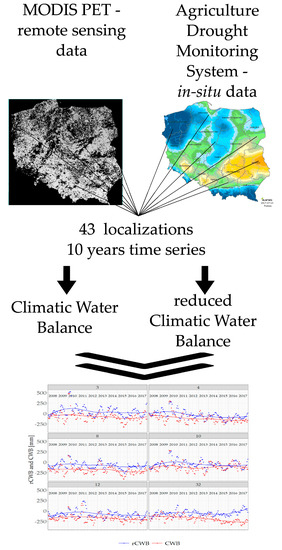
Graphical Abstract

1. Introduction

Drought is one of the main adverse phenomena affecting the efficiency of agricultural production in local and global terms [1,2]. In addition to the direct impact on food production on a global scale, drought also has a huge impact on the economies of countries affected by this threat [3,4]. Drought as a meteorological phenomenon occurs with varying intensity in subsequent years in different regions. This applies in particular to areas located in the transitional climate zone. For this reason, monitoring drought and adapting agricultural production to its conditions is extremely crucial for countries where agriculture is an important branch of the economy. Poland is the leading agricultural producer in Central Europe, where more than 60% area (>146,000 km2) was adopted as agricultural land. The agricultural sector in Poland has a significant impact on the development and stability of the economy [5]. In Europe, Poland is one of the main producers of cereal, potato and apple—providing in 2017 10.1%, 18.2% and 20.0% of the total EU output, respectively [6]. On the other hand, a long-time analysis revealed that, in extreme cases, even half of the rural areas in Poland can be affected by agricultural drought [7], making this threat an underlying problem of Polish agriculture. From that point of view, the permanent monitoring of water resources has to be performed for the entire territory of Poland with the best time and spatial precision possible.
In order to observe water balance and forecast agricultural drought, different indicators may be applied [8]. One of the models often used in drought indicators and indices is the water balance model [8]. It measures balance between water demand, measured by evapotranspiration (ET), and water supply, measured by precipitation. ET is a combination of two separate processes, whereby water is lost through evaporation from the soil and plant surface on the one hand and, on the other hand, via transpiration from the aboveground parts of plants. When the crop is small, water is predominately lost through soil evaporation, but once the crop is well developed and completely covers the soil, transpiration becomes the main process [9].
Currently in the world, several national monitoring systems are being developed, which use different indicators to qualify the phenomenon of agricultural drought in a given area, depending on the type of input data and their origin [10,11] In the case of Poland, the reduced Climatic Water Balance (rCWB) is the basic indicator to estimate the water available for plants. The rCWB is published in the frame of the Agricultural Drought Monitoring System (ADMS) developed by the Institute of Soil Science and Plant Cultivation—State Research Institute (IUNG), according to the methodology consistent with the requirements of Polish law [12,13]. The rCWB defines how much water is available for plants and is derived from two parameters: precipitation (P) and potential evaporation (PE) [9] where the Penman concept [14] was used for PE assessment. Both inputs are assessed based on meteorological data measured on ground metrological stations, provided by the Institute of Meteorology and Water Management—National Research Institute (IMGW) supported by additional measuring locations of the ADMS meteorological net. While precipitation measurements are well established and provided for more than 660 localizations across Poland, the estimation of PE is more difficult, basically because of the small number of stations with solar radiation flux measurement abilities (only 58 synoptic stations in 2018 are equipped with dedicated devices). Comprehensive information about the system, methodology and the obtained results from 2008–2018 is available on the website [15].
To fully describe the water resources reduction in soil, a plants transpiration effect should be taken into account and the potential evapotranspiration (PET) parameter should be assessed. There is a variety of formulas for PET values estimation—e.g., combination method [14,16], radiation-based method [17] or temperature-based method [18]. All of them are well adopted for ground meteorological stations’ inputs. Remote sensing Earth observations, that have been strongly developed in recent years, give the opportunity of employing a new perspective for PET estimation on a global as well as local scale. As a significant example, the mission of twin satellites Terra and Aqua should be indicated. The Moderate Resolution Imaging Spectroradiometer (MODIS) modules installed on the abovementioned satellites provide the datasets necessary for the final product of PET with an 8-day temporal and 500 m spatial resolution [19]. The algorithm of MODIS was based on the Penman–Monteith concept. Using the PET values, it is possible to evaluate the Climatic Water Balance (CWB) indicator that is expressed as the difference between precipitation and PET (in analogy to rCWB).
Taking into the advantages of satellite data, especially their spatial and temporal resolution, it is natural to implement these data into the national system of agricultural drought monitoring. The motivation for performed research was to assess the possibility for direct application of particular remote sensing data of PET from MODIS into the Agricultural Drought Monitoring System of Poland. Therefore, the objective of conducted research was to assess the impact of remote sensing PET from MODIS data application for results of Climatic Water Balance indicator used for agriculture drought assessment for territory of Poland. The presented research focused therefore on the comparison between:
(i)
The currently established in Poland methodology for the rCWB assessment which employed ground-based meteorological station data;
(ii)
The CWB obtained using rainfall from ground stations plus remote sensing values of PET from MODIS instrument.

2. Materials and Methods

2.1. Input Data, Spatial and Temporal Scale

The detailed list of data evaluated in the research is presented in Table 1. The remote sensing data were limited to potential evapotranspiration (denoted as PET) from MODIS instrument. The methodology for rCWB calculation using meteorological data was established and implemented by IUNG and in the presented work only the final product of rCWB was evaluated. From raw meteorological data only the precipitation (P) was investigated, as required for CWB computation. The studies for CWB were performed for the area of Poland, presented in Figure 1, considering a 10 year period from 2008 to 2017. For each year, thirteen specific periods (R) were computed according to the methodology implemented in the Agricultural Drought Monitoring System [15]. The reporting regime of ADMS was based on six-decade periods with a 10-day moving window starting from 1st April (Table 2). To avoid filling the missing data, only results obtained for specific localizations with full (i.e., continuous) ten years’ data for precipitation were evaluated. In total, 43 localizations were investigated. The distribution of stations was selected in such a way that they represent all types of main forms of land cover occurring in Poland.

2.2. Precipitation–P8

The precipitation data were obtained using the free access IMGW database in ASCII format [20]. The original one-day average precipitation values were summed to 8-day blocks to be consistent with the time scale of the PET product from MODIS.

2.3. Reduced Climatic Water Balance—rCWB

Agricultural drought in ADMS is determined using the reduced Climate Water Balance (rCWB), which is the difference between atmospheric precipitation and potential evaporation:
r C W B   = P 8 P E
where:
P8—sum of atmospheric precipitation for 8 days (mm);
PE—potential evaporation for 8 day period (mm).
The potential evaporation value is calculated on the basis of the simplified Penman [14] equation:
P E   =   161 + 19.57   d 152.7   l n ( d ) + 0.0004034   h 2 + 0.00187 ( t + 5 ) 3 + 0.004192 ( 100 f ) 2 + 0.0003681   v   ( 100 f ) 2.5
where:
d—length of the day (h);
h—sunshine (h);
t—average air temperature, (°C);
f—relative humidity at 12 GMT (%);
v—average wind speed, (m s−1).
Simplification of Penman’s formula resulted from the need to adapt the algorithm to the availability of meteorological data at the time when the system was created. In that period (2007–2008), the registration of all required weather phenomena was conducted by IMGW at about 50 synoptic meteorological stations.
ADMS is based on thirteen reporting periods, as presented in Table 2.

2.4. Potential Evapotranspiration from MODIS–PET

Moderate Resolution Imaging Spectroradiometer (MODIS) [21] is one of the 65 instruments mounted on Terra and Aqua twin satellites. MODIS provides data from 36 spectrometric bands covering wavelengths from 0.4 to 14.4 µm. The data from MODIS, depending on the specific band, are provided with the spatial resolutions of 250, 500 or 1000 m and are freely available on Land Processes Distributed Active Archive Centre [22]. One of the MODIS products (MOD16A2) is a package of four parameters including global potential evapotranspiration (denoted in the presented work as PET) for 8-day averaged values [19]. The data from PET are provided with a spatial resolution of 500 m. For the purpose of presented studies, the data MOD16A for the region of Poland covered by three swaths h18v03, h19v03, h19v04 were used. The algorithm for PET computation from remote sensing data in MODIS was based on Penman–Monteith model [14,16]. In addition, according to the MODIS algorithm [23] the PET calculation distinguished the evaporation from saturated soil and evaporation from the moist soil surface. The full algorithm for computation of PET from MODIS observation includes the input data obtained by the instrument as well as meteorological data provided by NASA’s Global Modelling and Assimilation Office (GMAO or MERRA GMAO) [24]. For the purpose of presented work, the results for PET were extracted from MOD16A products for 43 localizations as an average of the nearest 9 pixels to the examined point using QGIS software, version 3.4 [25].

2.5. Climatic Water Balance—CWB

Climatic Water Balance (CWB), which is the difference between atmospheric precipitation and potential evapotranspiration:
C W B   =   P P E T
where:
P—atmospheric precipitation (mm);
PET—potential evapotranspiration (mm).
Values of CWB for thirteen periods per year were calculated according to the simplified equation:
C W B R i = R i P 8 R i P E T
For the particular period Ri, the summation represents the operation on all 8-day datasets for P8 and PET within the day of the year (DoY) for CWB, as presented in Table 2. Because of differences in time coverage, the shift for the period Ri for rCWB and CWB equaled 4 days at maximum and was assumed to be negligible compared to the 60-day periods. The 4-day shifts were noted for the starting day for periods R2, R6 and R10, as well as for ending day for periods R4 and R11.

2.6. Data Analysis

The results obtained with rCWB and CWB were analyzed using four indicators: Pearson’s correlation coefficient (r), root mean square error (RMSE) [26], mean absolute error (MAE) [26] and Mann–Kendall statistic Z-index (Z).
In order to avoid the uncertainty related to interpolations, all presented calculations were performed on the data from 43 mentioned localizations. Results of rCWB and CWB values for ten years for particular localization j represent time series objects. The data were presented in two approaches. First, they were shown as a classical time series with one-period (R) step, then data were grouped according to periods. In addition, for better visualizations, data were averaged and expressed by curves obtained using a smoothing method with a local polynomial regression fitting approach [27]. In order to investigate the agreement for rCWB and CWB, the set of analyses were performed with three explicit steps:
Step 1: The statistical test including Pearson’s correlation coefficient (r), root mean square error (RMSE) and mean absolute error (MAE) (the equations for evaluation r, MAE and RMSE are included in Appendix A) were evaluated as being representative for a similar investigation [28,29,30];
Step 2: The accuracy of data grouped in periods was represented by subtraction of the rCWBj,Ri and CWBj,Ri for a particular localization j and period Ri. The result was presented as a mean value for 10 years:
S j , R i   =   a r C W B a , j , R i C W B a , j , R i 10
where Sj,Ri denotes mean value from subtraction result for localization j and period Ri and a represents the year of observation (2008–2017);
Step 3: The agreement of trend monotony for rCWB and CWB was evaluated. The test using the nonparametric Mann–Kendall method [31,32], computed with “MannKendall’ package in R software [33] has been chosen for that purpose. The test is based on the statistics of the number of results with a positive and negative sign obtained from subtracting the subsequent values, chronologically following measurements in the time series. In the presented study, the considered data are the following results of the rCWB and CWB in time series, denoted as CWBx. For consecutive elements CWBx, we determined the sign of their subtraction sign (CWBx+1CWBx). We ascribed the sign (CWBx+1CWBx) function the value equal to −1 for results (CWBx+1CWBx) < 0, 0 for (CWBx+1CWBx) = 0 and +1 for (CWBx+1CWBx) > 0. The Mann–Kendall statistic Z for n observations and for particular localization j was calculated according to the equation:
Z j   =   x   =   1 x   =   n 1 s i g n ( C W B x + 1     C W B x )
The test covers the evaluation of Zj parameter that indicates an increasing trend when Zj > 0 and a decreasing trend with Zj < 0. Basing on the performed analysis the group of six localizations was presented and is discussed in following section. The group included localizations with the highest and the lowest r coefficient of the localization, with the highest revealed difference between rCWB and CWB and the localizations with well visualized drought and wet periods.

3. Results

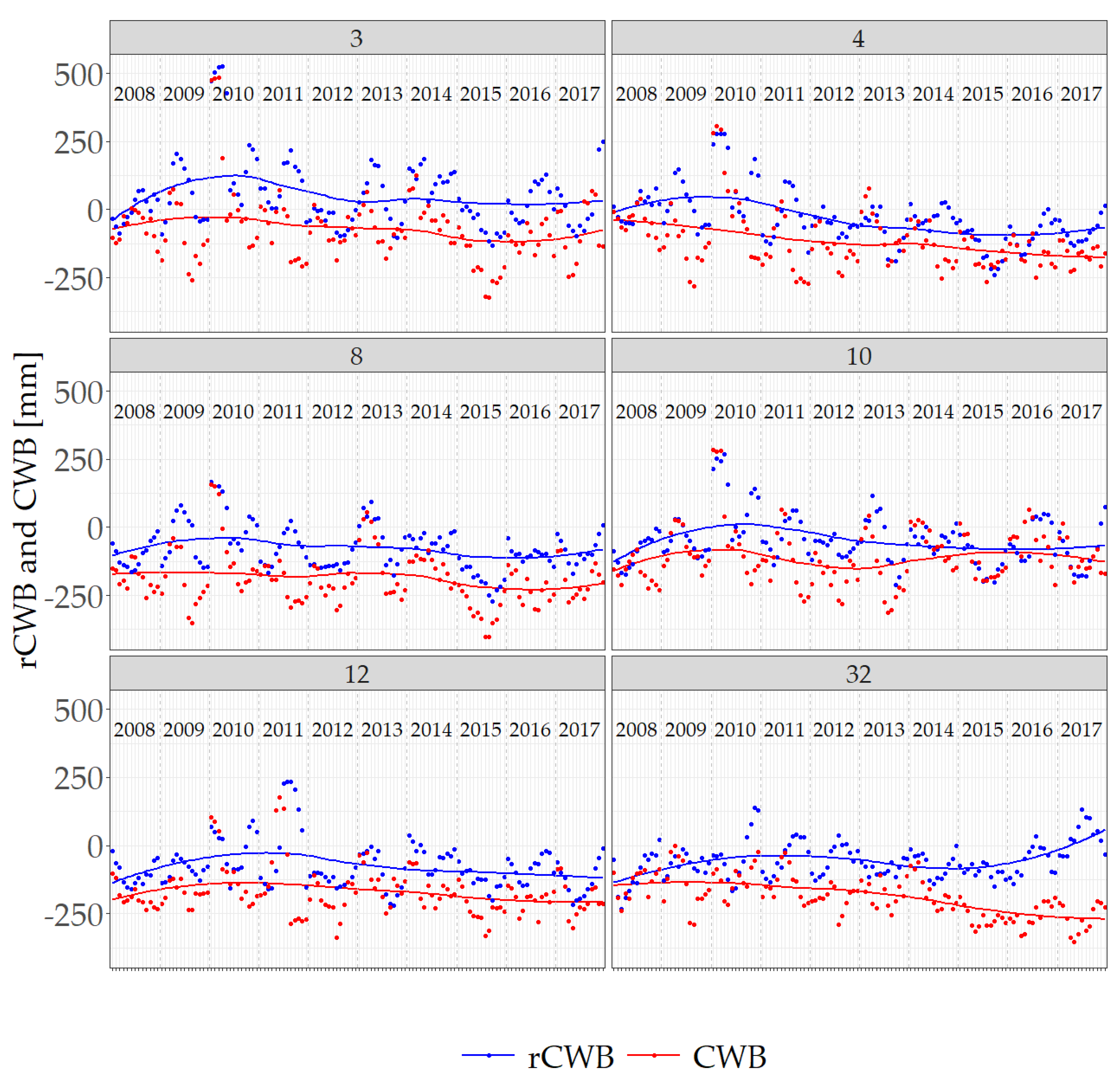
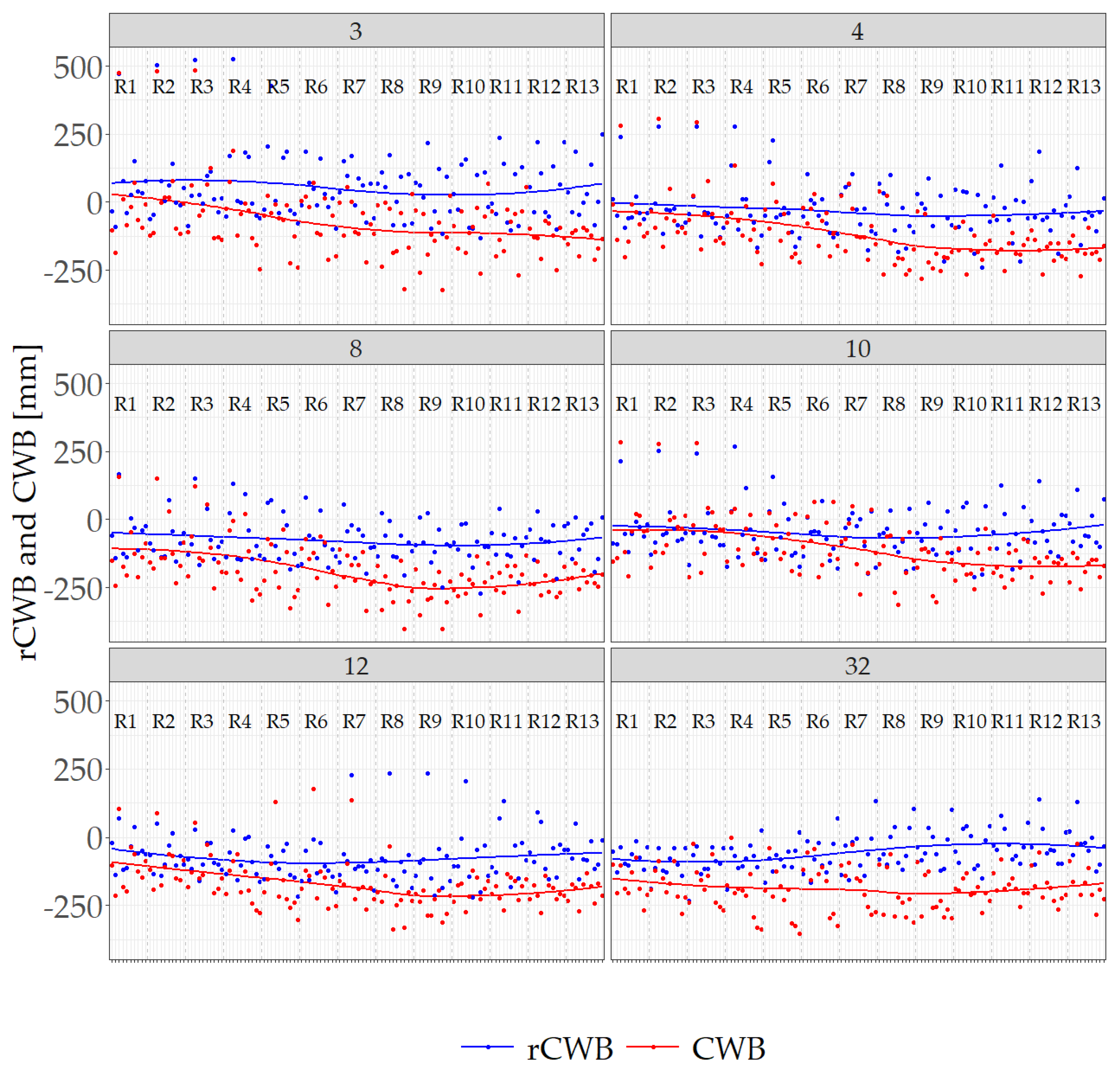
Time series of rCWB and CWB for six localizations and 10 years from 2008 to 2017 are presented in Figure 2 (results including the time series, trends in dependent on periods as well as correlations for all 43 analyzed localization can be found in Appendix B). The graphs include the results of smoothing as blue and red lines for a better visualization of long-time fluctuation. The smoothed lines visualize the tendency with lower CWB values from the long-time perspective. The evidence of drought—see localizations 3 and 8 for 2015—and extremely wet periods—see beginning of 2010 year for localizations 3, 4 and 10—are visualized. In some cases, good agreement of rCWB and CWB values was noted in extreme conditions as in 2010 when the wet conditions were observed for localizations 3, 4, 8 and 10 in Figure 2. On the other hand, the significant disagreement between rCWB and CWB, including the opposite trends, was observed, especially visible for all locations in 2011 for periods R7–R13. In extreme situations disagreement was higher than 500 mm, as in case of localization 12.
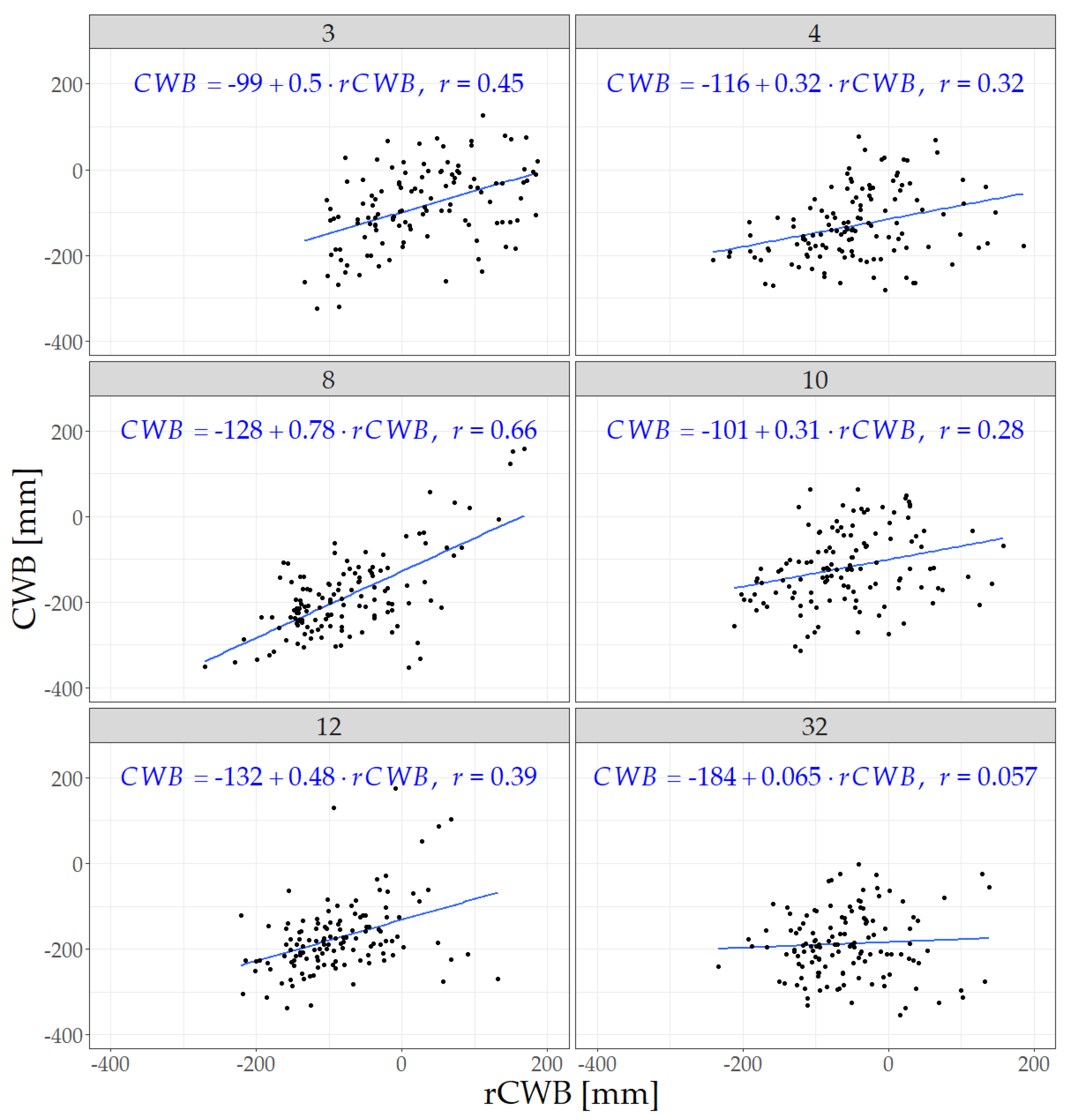
The correlation coefficients were determined as quantitative indicators of the compliance of the time series for each location. The correlation coefficients r for all evaluated localizations vary in the range from 0.06 (localization 32) to 0.68 (localization 8) and are presented in Appendix B. The correlation graphs for six localizations are presented in Figure 3. The particular graph presented in the figure was evaluated based on 130 data points (including 10 years and 13 reporting periods per year). The tendency with lower values of CWB comparing to rCWB was observed for all considered localizations.
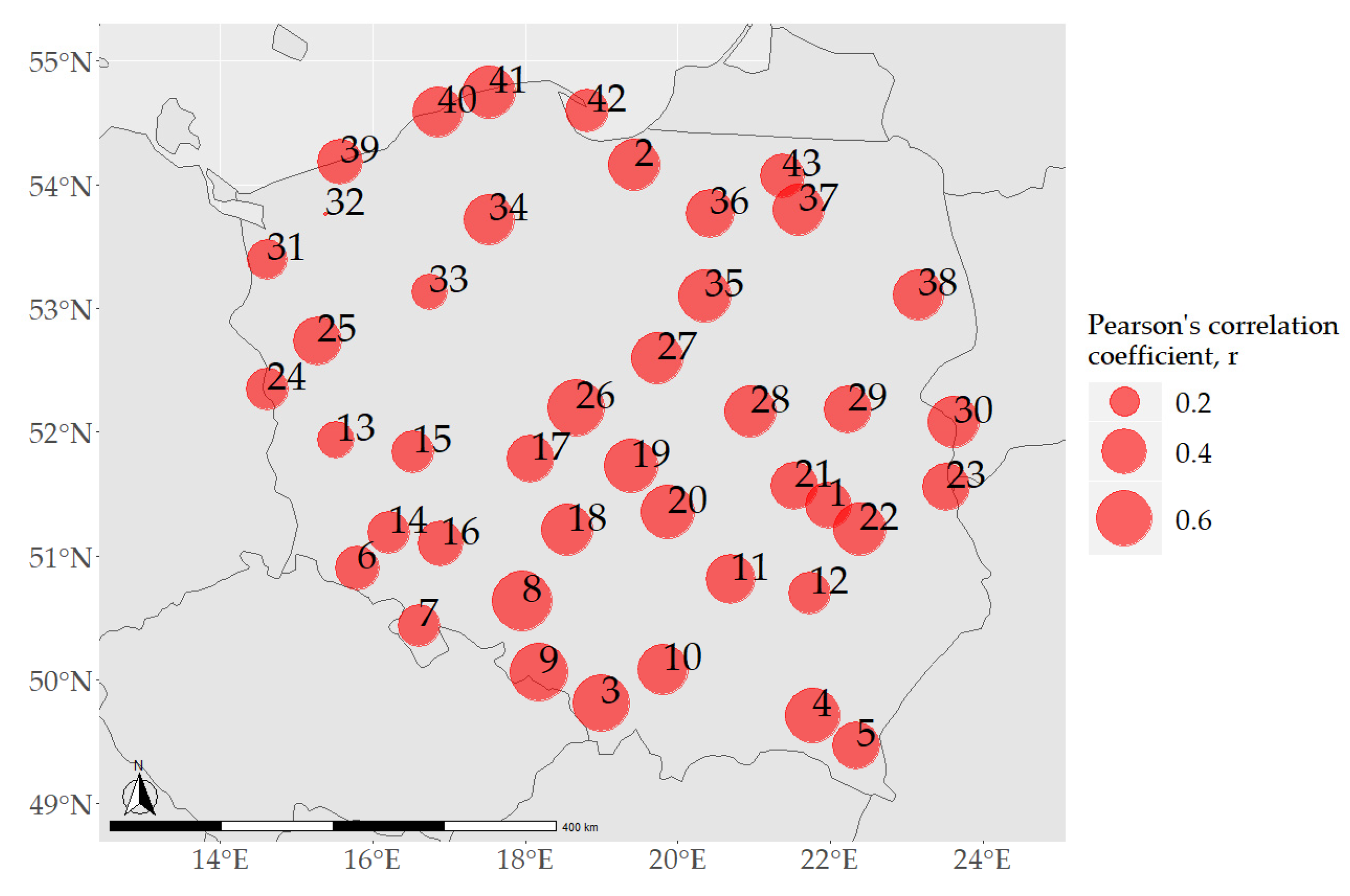
Considering the spatial distribution of r coefficients presented in Figure 4, higher correlations were observed for the locations in the belt from South–Central to North–Central Poland. The correlation coefficients for that sub-region were predominantly higher than 0.5 with the maximum value of 0.66 for localization 8. As one can see, in general, the lower correlations were observed in the western region of the country, where r ranged from 0.06 to 0.49. The lowest value was observed for the localization in the North–Western part of Poland—localization 32. On the country scale, the most common correlation coefficient was 0.5.
Considering the CWB fluctuation, depending on the reporting period, as presented for six localizations in Figure 5, we observe a more stable waveform for rCWB indices. The values of CWB highlight the decreasing tendency from period R8, being well visualized by smoothing curves, and, as was confirmed, by Sj,Ri indicator test, presented in Figure 6a.
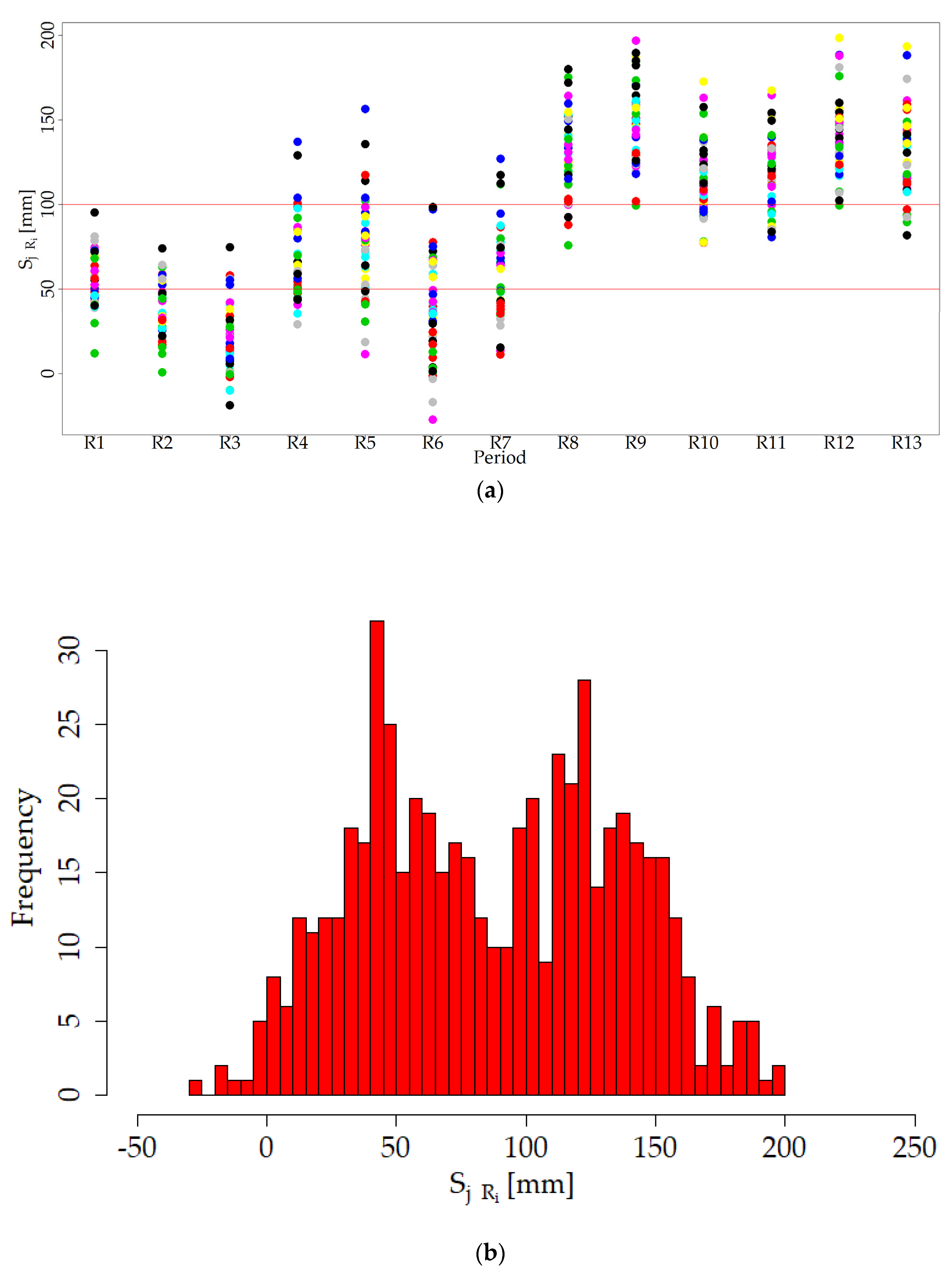
The indicator Sj,Ri significantly depends on the period of the year. Results presented in Figure 6 show that on average Sj,Ri values increase as we move towards the later periods with a clearly visible break point between R7 and R8 that falls at the end of May (close to 160 DoY). The highest Sj,Ri with values closest to 200 mm were observed for periods R9 and R12. In addition, for periods R4 and R5, most localizations are characterized by Sj,Ri higher than 50 mm, while for periods R8–R13, most Sj,Ri values lie above 100 mm. Results shown in the Figure 6 provide two main points: first, the change in mean values (the average: j S j , R i 43 ) of the Sj,Ri for a particular period indicates time-dependent fluctuations associated with the vegetation cycle or climatic behavior for Poland; second, discrepancies in Sj,Ri values within a given period provide the information about fluctuation on spatial distribution of Sj,Ri. As we can see, both the significant sensitivity of Sj,Ri for time-dependent impact, as well as for spatial distribution, were observed. The histogram in Figure 6b shows two clearly observed maxima for values around 45 mm and 125 mm. The first value is the most probable for periods from R1 to R7; the second one for periods from R8 to R13. Concluding, for periods in the second half of the year, Sj,Ri indicators increased almost threefold. Considering the spatial distribution, it was shown that the spatial fluctuation of Sj,Ri was almost constant and the spread of the Sj,Ri values in relation to the average was close to ±50 mm, regardless of the period.
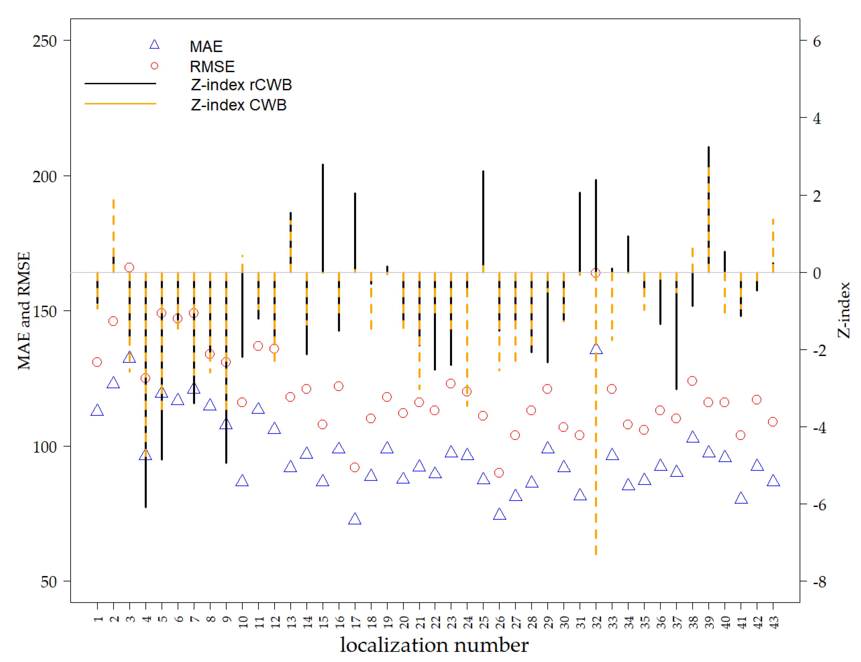
The highest RMSE and MAE (170 mm and 142 mm, respectively) were observed for localization, with the smallest r value, and it was localized in the north-western part of Poland (No. 32). For that location, the highest discrepancy for Z-index indicator for rCWB and CWB was obtained as well. The lowest errors were reported for localization 26, where the values of 88 mm and 75 mm were assessed, respectively, for RMSE and MAE.
Considering the variance of the Z-index, it was observed that the simultaneous negative indicator value for rCWB and CWB was recorded for 28 stations, and only for six cases was it simultaneously positive. In nine cases, the sign of the Z-index was inconsistent for rCWB and for CWB. In addition, except for the localization, 32 were already indicated as having the higher RMSE and MAE. Figure 7 clearly shows a group of locations with significantly elevated RMSE and MAE values—10 localizations on the left side of the graph (1 to 12, excluding 4 and 10).

4. Discussion

Performed research revealed the strong inconsistency between rCWB and CWB indicators. As we observed, the disagreements were higher for warmer periods in the year, giving the evidence that vegetation presence has a significant impact on the potential evapotranspiration process. The data could have an important impact regarding the issue of evaluating the dependence between the vegetation cover and level of evapotranspiration, as recently discussed by Wang et al., 2018 [34]. In addition, the increase in differences between rCWB and CWB were observed for periods when extreme events, such as drought and high precipitation take place. When analyzing the obtained data in terms of spatial distribution, it can be observed that the lowest correlation of rCWB and CWB values occurs in the western part of Poland. This is the area that is most severely affected by agricultural drought each year, according to data published by IUNG [15].
In the context of applicability of PET remote sensing data from MODIS to the ADMS, we observed that, in the case of direct application of satellite data, we should deal with the error at the level of around 100 mm with simultaneous CWB at the level around the −50 mm mark, which gives an unacceptable condition. The results are in contrast with conclusions presented by Caccamo et al., 2011 [35], who proved that the involvement of MODIS data can give accurate results for assessing the agricultural drought, even for regions with dense vegetation. In our case, as was also presented and discussed by Bormann 2011 [36] the significant impact for Climatic Water Balance assessment have the model used for PET calculation. Considering the model was used to determine PET from data obtained from the MODIS instrument, it should be noted that one of the components of this model is related directly to the vegetation index—i.e., LAI (Leaf Area Index). In contrast, the model used for rCWB is not sensitive for vegetation. In the ADMS, vegetation impact is taken into account at the final step of agricultural drought assessment by referring the calculated rCWB to the decision levels for particular vegetation type. In addition, the process of evapotranspiration is affected by the availability of water in soils. In conclusion, two parameters were introduced as possibly having a direct relation to the phenomena of increasing Sj,Ri parameter observed from R7 in presented results. Firstly, as the beginning of the R7 period falls on 150 DoY—i.e., the end of May—the vegetative cycles of plants (expressed as LAI) should be considered. Secondly, the soil moisture (SM) that could express the climatic behavior in the area of Poland have to be taken into account
The decreasing trend assessed both for rCWB, as well as for CWB for most of localizations, indicates the propagation of drought condition for the majority of areas in Poland. We should compare the results with the conclusions of McCabe and Wolock, 2015 [37] which investigated the global trend of drought based on the differences of P and PET and with the results of the Mann–Kendall test performed for CWB, assessed for particular localizations in Romania presented by Bandoc and Prăvălieat, 2015 [38]. McCabe and Wolock [37] considered 100 year periods, computing percentage of global land area affected by drought conditions. As they concluded, in the long period, the problem of increasing temperature that has direct influence on the increase in PET was compensated by increasing precipitation, so the mean value of the drought index has no significant impact on trend.
From the other site for Romania localization, presented by Bandoc and Prăvălieat [38], the negative trend was observed for only four localizations with simultaneous positive trends for the five other locations. In our research, the negative trend was observed for 28 localizations and only six localizations revealed positive trends.

5. Conclusions

The presented results clearly indicate that, due to the high values of obtained error indicators (MAE and RMSE) and low correlation between two investigated indicators, they do not allow for the direct integration of satellite PET from MODIS data into the ADMS. The conducted research shows that the integration of PET satellite data from the MODIS system with the ground-based agricultural drought monitoring system in Poland is possible only after the appropriate modification of the rCWB index determination method.
An important observation coming from the presented results is the fact that, during the data integration procedure, particular attention should be paid to the climatic characteristics of the given area for which such data integration is carried out. The example of Poland shows that the possibility of integrating specific data may be associated not only with the characteristics of the terrain (land relief) but also, if not mainly, with the periodicity during the year associated with changes in the weather conditions and the presence of vegetation; however, this issue should be investigated in more detail in the future research..

Author Contributions

Conceptualization: K.S., H.Ł. and Ł.G.; Data curation: R.P., A.D. and J.S.; Formal analysis: H.Ł. and K.S.; Funding acquisition: M.Ł. and B.U.; Methodology: K.S. and H.Ł.; Supervision: B.U.; Writing—original draft: K.S., H.Ł., R.P., A.D. and A.R.-P.; Writing—review and editing: H.Ł., K.S., R.P., A.D., M.Ł. and A.R.-P. All authors have read and agreed to the published version of the manuscript.

Funding

This research was funded by the Polish National Centre for Research and Development (grant number: BIOSTRATEG3/345940/7/NCBR/2017) and the Polish Ministry of Agriculture and Rural Development (grant number: F.gr. 442.9.2018).

Acknowledgments

We would like to thank Małgorzata Wydra for her help with editing the English manuscript of this paper.

Conflicts of Interest

The authors declare no conflict of interest. The funders had no role in the design of the study; in the collection, analyses, or interpretation of data; in the writing of the manuscript, or in the decision to publish the results.

Appendix A

r = i = 1 n ( C W B C W B ¯ ) · ( r C W B r C W B ¯ ) i = 1 n ( C W B C W B ¯ ) 2 · i = 1 n ( r C W B r C W B ¯ ) 2 ,
M A E = i = 1 n ( r C W B C W B ) n ,
R M S E = i = 1 n ( r C W B C W B ) 2 n ,

Appendix B

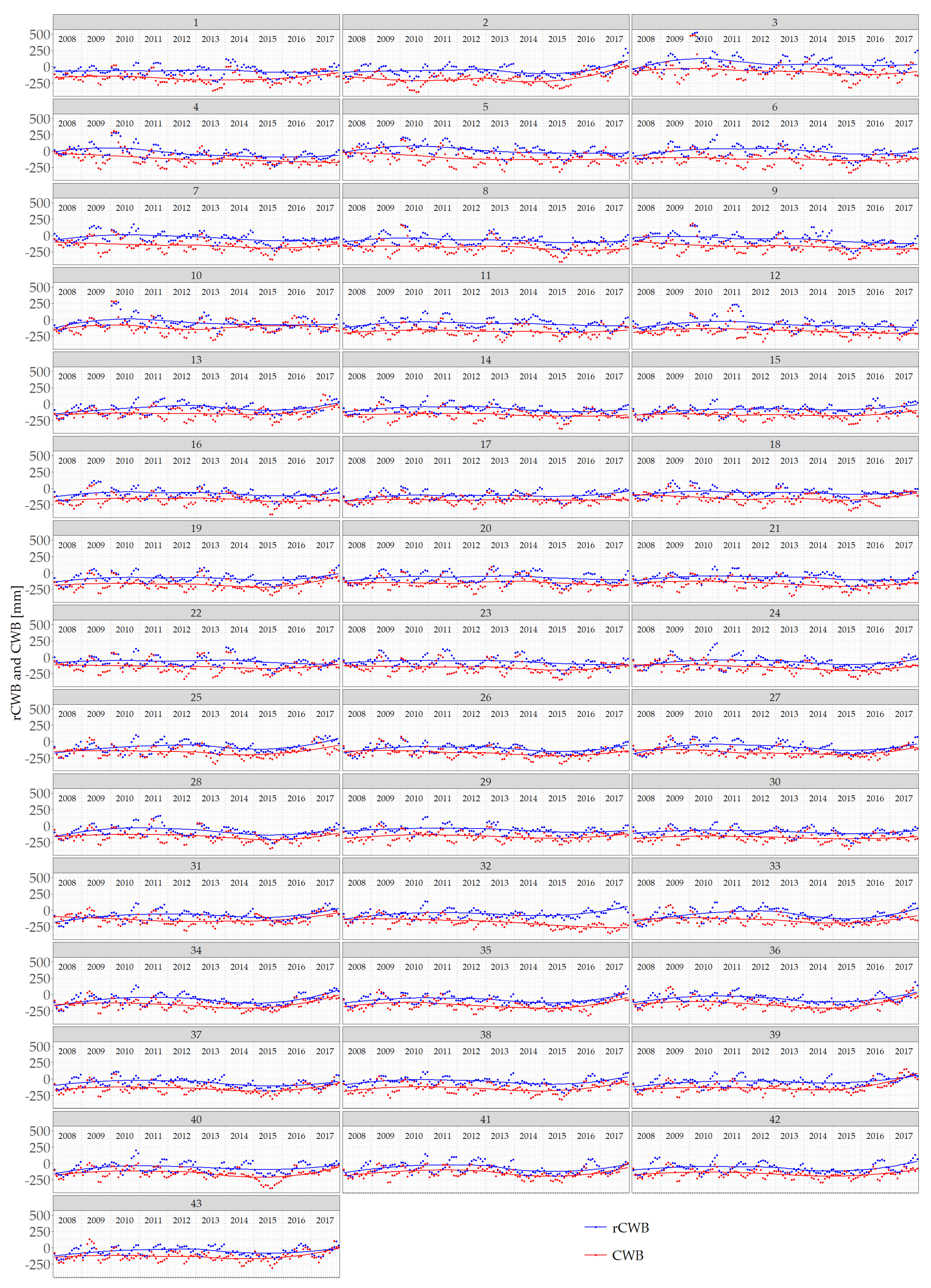
Figure A1. Time series of rCWB and CWB for 10-year period (2008–2017). The solid red and blue lines represent the smoothing result.
Remotesensing 12 03411 g0a1
Figure A2. The fluctuation of rCWB and CWB for a 10-year time scale (2008–2017) presented as function of periods (R1–R13)—10 data points for each period Ri for 43 analyzed localizations. A particular graph represents one localization. The solid red and blue lines represent the smoothing result.
Remotesensing 12 03411 g0a2
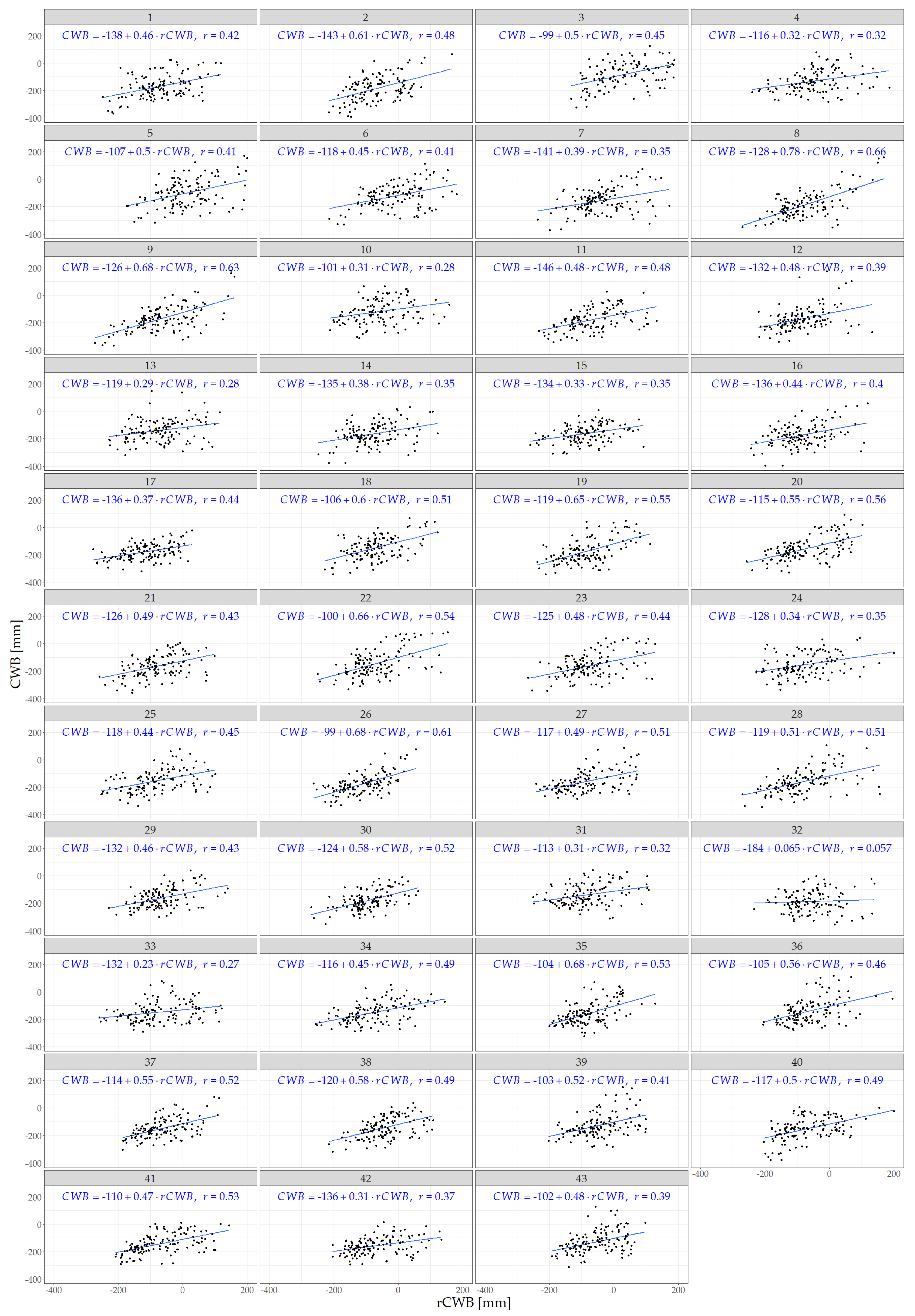
Figure A3. Correlation of rCWB and CWB for 43 localization across the Poland with regression line (blue line) and correlation coefficients r. Data obtained for 10 years with 13 periods for each year (130 data points for each localization).
Remotesensing 12 03411 g0a3

References

  1. Gornall, J.; Betts, R.; Burke, E.; Clark, R.; Camp, J.; Willett, K.; Wiltshire, A. Implications of climate change for agricultural productivity in the early twenty-first century. Philos. Trans. R. Soc. B Biol. Sci. 2010, 365, 2973–2989. [Google Scholar] [CrossRef] [PubMed]
  2. Yu, C.; Huang, X.; Chen, H.; Huang, G.; Ni, S.; Wright, J.S.; Hall, J.; Ciais, P.; Zhang, J.; Xiao, Y.; et al. Assessing the impacts of extreme agricultural droughts in China under climate and socio-economic changes. Earth’s Future 2018, 6, 689–703. [Google Scholar] [CrossRef]
  3. European Commission. Third Follow up Report to the Communication on Water Scarcity and Droughts in the European Union COM (2007) 414 Final; European Commission: Brussels, Belgium, 2011. [Google Scholar]
  4. Armenski, T.; Stankov, U.; Dolinaj, D.; Mesaros, M.; Jovanovic, M.; Pantelic, M.; Pavic, D.; Popov, S.; Popovic, L.; Frank, A.; et al. Social and economic impact of drought on stakeholders in agriculture. Geogr. Pannonica 2014, 18, 34–42. [Google Scholar] [CrossRef] [Green Version]
  5. Borek, D.; Głowacka-Smolis, K.; Gustyn, J.; Kozera, A.; Kozłowska, J.; Lipowska, E.; Marikin, M.; Nowak, T.; Pilaszek, K.; Rybak-Nguyen, E.; et al. Statistical Yearbook of the Republic of Poland; Statistics Poland: Warsaw, Poland, 2018.
  6. European Commission—EUROSTAT. Available online: https://appsso.eurostat.ec.europa.eu/nui/show.do?dataset=apro_cpsh1&lang=en (accessed on 15 October 2020).
  7. Somorowska, U. Changes in Drought Conditions in Poland over the Past 60 Years Evaluated by the Standardized Precipitation-Evapotranspiration Index. Acta Geophys. 2016, 64, 2530–2549. [Google Scholar] [CrossRef] [Green Version]
  8. Svoboda, M.; Fuchs, B. Handbook of Drought Indicators and Indices. World Meteorological Organization (WMO) and Global Water Partnership (GWP). Integrated Drought Management Programme (IDMP). Integrated Drought Management Tools and Guidelines. Series 2. 2016. Available online: https://www.drought.gov/drought/sites/drought.gov.drought/files/GWP_Handbook_of_Drought_Indicators_and_Indices_2016.pdf (accessed on 15 October 2020).
  9. Allen, R.G.; Pereira, L.S.; Raes, D.; Smith, M. Crop evapotranspiration-Guidelines for computing crop water requirements—FAO Irrigation and drainage. Tech. Rep. 1998, 300, D05109. [Google Scholar]
  10. Zink, M.; Samaniego, L.; Kumar, R.; Thober, S.; Mai, J.; Schäfer, D.; Marx, A. The German drought monitor. Environ. Res. Lett. 2016, 11, 74002. [Google Scholar] [CrossRef]
  11. Donald, W. Drought as a Natural Hazard: Concepts and Definitions. Drought, a Global Assessment. 1. 2000. Available online: https://www.researchgate.net/publication/243785200_Drought_as_a_Natural_Hazard_Concepts_and_Definitions (accessed on 15 October 2020).
  12. Doroszewski, A.; Jadczyszyn, J.; Kozyra, J.; Pudełko, R.; Stuczyński, T.; Mizak, K.; Łopatka, A.; Koza, P.; Górski, T.; Wróblewska, E. Podstawy systemu monitoringu suszy rolniczej. Woda-Środowisko-Obszary Wiejskie 2012, 12, 77–91. [Google Scholar]
  13. The Government of Republic of Poland. The Act of 7 July 2005 on Insurance of Agricultural Crops and Livestock. J. Law 2005, 150, 1249. [Google Scholar]
  14. Penman, H.L. Natural evaporation from open water, bare soil and grass. Proc. R. Soc. Lond. Ser. A Math. Phys. Sci. 1948, 193, 120–145. [Google Scholar]
  15. ADMS. Web-Portal of Agricultural Drought Monitoring System Institute of Soil Sciences and Plant Cultivation—State Research Institute, 2008–2019. 2019. Available online: www.susza.iung.pulawy.pl (accessed on 15 October 2020).
  16. Monteith, J.L. Evaporation and environment. Symp. Soc. Exp. Biol. 1965, 19, 205–234. [Google Scholar]
  17. Priestley, C.H.B.; Taylor, R.J. On the assessment of surface heat and evaporation using large-scale parameters. Mon. Weather Rev. 1972, 100, 81. [Google Scholar] [CrossRef]
  18. Thornthwaite, C.W. An approach toward a rational classification of climate. Geogr. Rev. 1948, 38, 55–94. [Google Scholar] [CrossRef]
  19. Running, S.W.; Mu, Q.; Zhao, M.; Moreno, A. MODIS Global Terrestrial Evapotranspiration (ET) Product (NASA MOD16A2/A3) NASA Earth Observing System MODIS Land Algorithm; NASA: Washington, DC, USA, 2017.
  20. Public Data Base IMGW-PIB. Available online: https://danepubliczne.imgw.pl/ (accessed on 15 October 2020).
  21. Salomonson, V.; Barnes, W.; Masuoka, E. Introduction to MODIS and an Overview of Associated Activities. Earth Sci. Satell. Remote Sens. 2006, 1, 12–32. [Google Scholar]
  22. Land Processes Distributed Active Archive Centre. Available online: https://lpdaac.usgs.gov (accessed on 15 October 2020).
  23. Mu, Q.; Zhao, M.; Running, S.W. Algorithm Theoretical Basis Document: MODIS Global Terrestrial Evapotranspiration (ET) Product (NASA MOD16A2/A3). Collection 5; NASA Headquarters: Washington, DC, USA, 2013.
  24. Schubert, S.D.; Rood, R.B.; Pfaendtner, J. An assimilated dataset for earth science applications. Bull. Am. Meteorol. Soc. 1993, 74, 2331–2342. [Google Scholar] [CrossRef] [Green Version]
  25. QGIS Development Team. QGIS Geographic Information System. Open Source Geospatial Foundation. 2009. Available online: http://qgis.osgeo.org (accessed on 15 October 2020).
  26. Wilmott, C.J.; Matsuura, K. Advantages of the mean absolute error (MAE) over the root mean square error (RMSE) in assessing average model performance. Clim. Res. 2005, 30, 79–82. [Google Scholar] [CrossRef]
  27. Cleveland, W.S.; Grosse, E.; Shyu, W.M. Local regression models. In Statistical Models in S (Wadsworth & Brooks/Cole); Chambers, J., Hastie, T., Eds.; CRC Press I Llc: Boca Raton, FL, USA, 1992. [Google Scholar]
  28. Al-Yaari, A.; Wigneron, J.P.; Ducharne, A.; Kerr, Y.; de Rosnay, P.; de Jeu, R.; Govind, A.; Bitar, A.A.; Albergel, C.; Munoz-Sabater, J.; et al. Global-scale evaluation of two satellite-based passive microwave soil moisture datasets (SMOS and AMSR-E) with respect to Land Data Assimilation System estimates. Remote Sens. Environ. 2014, 149, 181–195. [Google Scholar] [CrossRef] [Green Version]
  29. Zeng, J.; Li, Z.; Chen, Q.; Bi, H.; Qiu, J.; Zou, P. Evaluation of remotely sensed and reanalysis soil moisture products over the Tibetan Plateau using in-situ observations. Remote Sens. Environ. 2015, 163, 91–110. [Google Scholar] [CrossRef]
  30. Cui, C.; Xu, J.; Zeng, J.; Chen, K.S.; Bai, X.; Lu, H.; Chen, Q.; Zhao, T. Soil moisture mapping from satellites: An intercomparison of SMAP, SMOS, FY3B, AMSR2, and ESA CCI over two dense network regions at different spatial scales. Remote Sens. 2018, 10, 33. [Google Scholar] [CrossRef] [Green Version]
  31. Mann, H.B. Non-parametric tests against trend. Econometrica 1945, 13, 163–171. [Google Scholar] [CrossRef]
  32. Kendall, M.G. Rank Correlation Methods, 4th ed.; Charles Griffin: London, UK, 1975. [Google Scholar]
  33. McLeod, A.I. Kendall Rank Correlation and Mann-Kendall Trend Test. R Package Kendall. 2005. Available online: http://www.stats.uwo.ca/faculty/aim (accessed on 15 October 2020).
  34. Wang, Y.; Liu, Y.; Jin, J. Contrast Effects of Vegetation Cover Change on Evapotranspiration during a Revegetation Period in the Poyang Lake Basin, China. Forests 2018, 9, 217. [Google Scholar] [CrossRef] [Green Version]
  35. Caccamo, G.; Chisholm, L.; Bradstock, R.; Puotinen, M. Assessing the sensitivity of MODIS to monitor drought in high biomass ecosystems. Remote. Sens. Env. 2011, 115, 2626–2639. [Google Scholar] [CrossRef]
  36. Bormann, H. Sensitivity analysis of 18 different potential evapotranspiration models to observed climatic change at German climate stations. Clim. Chang. 2010, 104, 729–753. [Google Scholar] [CrossRef]
  37. McCabe, G.J.; Wolock, D.M. Variability and trends in global drought. Earth Space Sci. 2015, 2, 223–228. [Google Scholar] [CrossRef]
  38. Bandoc, G.; Prăvălie, R. Climatic water balance dynamics over the last five decades in Romania’s most arid region, Dobrogea. J. Geogr. Sci. 2015, 25, 1307–1327. [Google Scholar] [CrossRef]
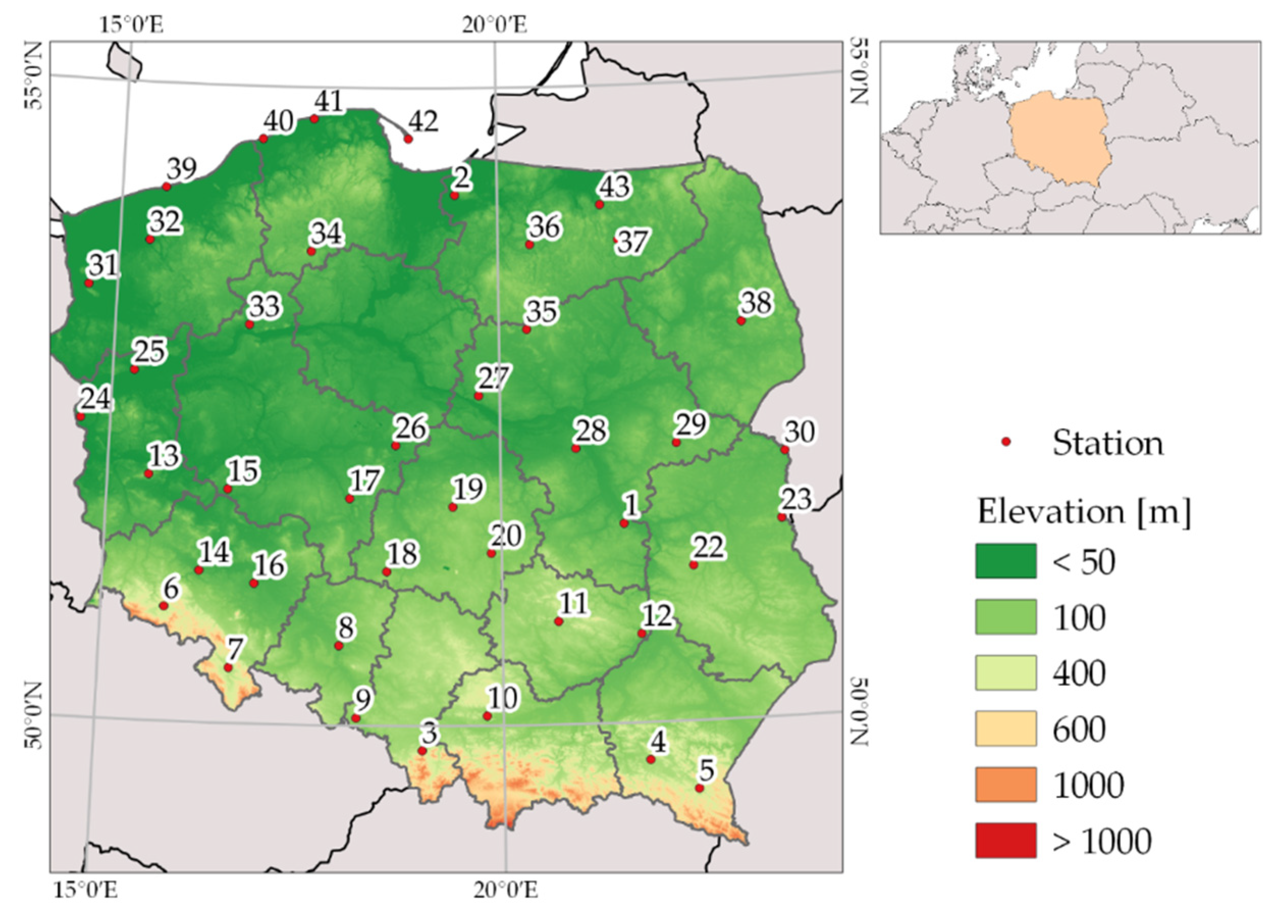
Figure 1. Study area with location of 43 meteorological stations used in this study. Background: Global Multi-resolution Terrain Elevation Data 2010 (provider: U.S. Geological Survey). IDs of the stations according to the register of the Polish public administration, Institute of Meteorology and Water Management—National Research Institute.
Remotesensing 12 03411 g001
Figure 2. Time series of rCWB and CWB for six localizations for 10-year period (2008–2017). The solid red and blue lines represent the smoothing result. The numbers in the headers of each graph represent the localization numbers consistent with data presented in Figure 1.
Remotesensing 12 03411 g002
Figure 3. Correlation of rCWB and CWB for six localization across Poland with regression line (blue line) and correlation coefficients r. Data obtained for 10 years with 13 periods for each year (130 data points for each localization).
Remotesensing 12 03411 g003
Figure 4. The spatial distribution of Pearson’s correlation coefficients (r), expressed as the dimension of point for particular localization.
Remotesensing 12 03411 g004
Figure 5. The fluctuation in rCWB and CWB for six localizations and for a 10-year time scale (2008–2017) presented as function of periods (R1–R13)—10 data points for each period Ri. The number in the header of each graph represents the localization number consistent with data presented in Figure 1. The solid red and blue lines represent the smoothing result.
Remotesensing 12 03411 g005
Figure 6. The fluctuation in Sj,Ri for 43 localizations (colour dots) as a function of periods R1–R13 (a), and the histogram of Sj,Ri indicators (b).
Remotesensing 12 03411 g006
Figure 7. Results for statistical tests including MAE (blue triangles), RMSE (red rings) and Mann–Kendall statistics (Z-index rCWB and Z-index CWB—black and orange bars, respectively) for 43 localization. The dashed (black-orange) lines represent localizations with consistent trends for Mann–Kendall test (positive or negative).
Remotesensing 12 03411 g007
Table 1. Input data evaluated for the purpose of performed research including the temporal and spatial resolution for particular data.
QuantitySymbolUnitData Temporal ResolutionData Spatial ResolutionRemarks
Precipitation, dailyPdaymm1 day43 not regular data points over PolandData for period I 2008–XII 2017
Precipitation, 8-daysP8mm8 days43 not regular data points over PolandSummation from 1-day precipitation data
Potential evapotranspiration from MODISPETmm8 days500 mRemote sensing product from MODIS
reduced Climatic Water Balance provided by IUNGrCWBmm6 decades43 not regular data points over Poland Provided for 13 periods per year with a 10-day moving window starting from 1st April
Climatic Water Balance computed from MODIS dataCWBmm8 weeks43 not regular localizations over Poland
Table 2. Time period adopted for rCWB and CWB calculation expressed as “Day of Year” (DoY).
Period DesignationReporting Period Implemented in ADMSReporting Period for rCWB (DoY) Reporting Period for CWB (DoY)
R11 IV–31 V91–15189–153
R211 IV–10 VI101–161105–161
R321 IV–20 VI111–171113–169
R41 V–30 VI121–181121–185
R511 V–10 VII131–191129–193
R621 V–20 VII141–201145–201
R71 VI–31 VII152–212153–209
R811 VI–10 VIII162–222161–225
R921 VI–20 VIII172–232169–233
R101 VII–31 VIII182–243185–241
R1111 VII–10 IX192–253193–249
R1221 VII–20 IX202–263201–265
R131 VIII–30 IX213–273211–271
Publisher’s Note: MDPI stays neutral with regard to jurisdictional claims in published maps and institutional affiliations.