Estimation of Organic Carbon in Anthropogenic Soil by VIS-NIR Spectroscopy: Effect of Variable Selection

 ,
, 
 ,
, 

Abstract
:
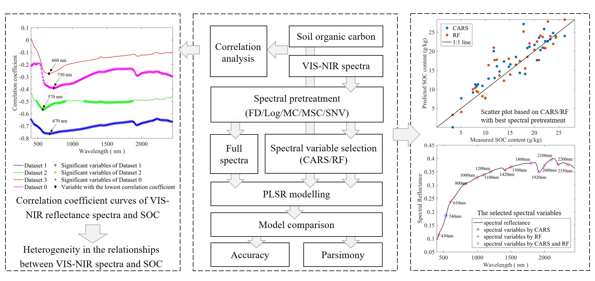
1. Introduction
2. Materials and Methods
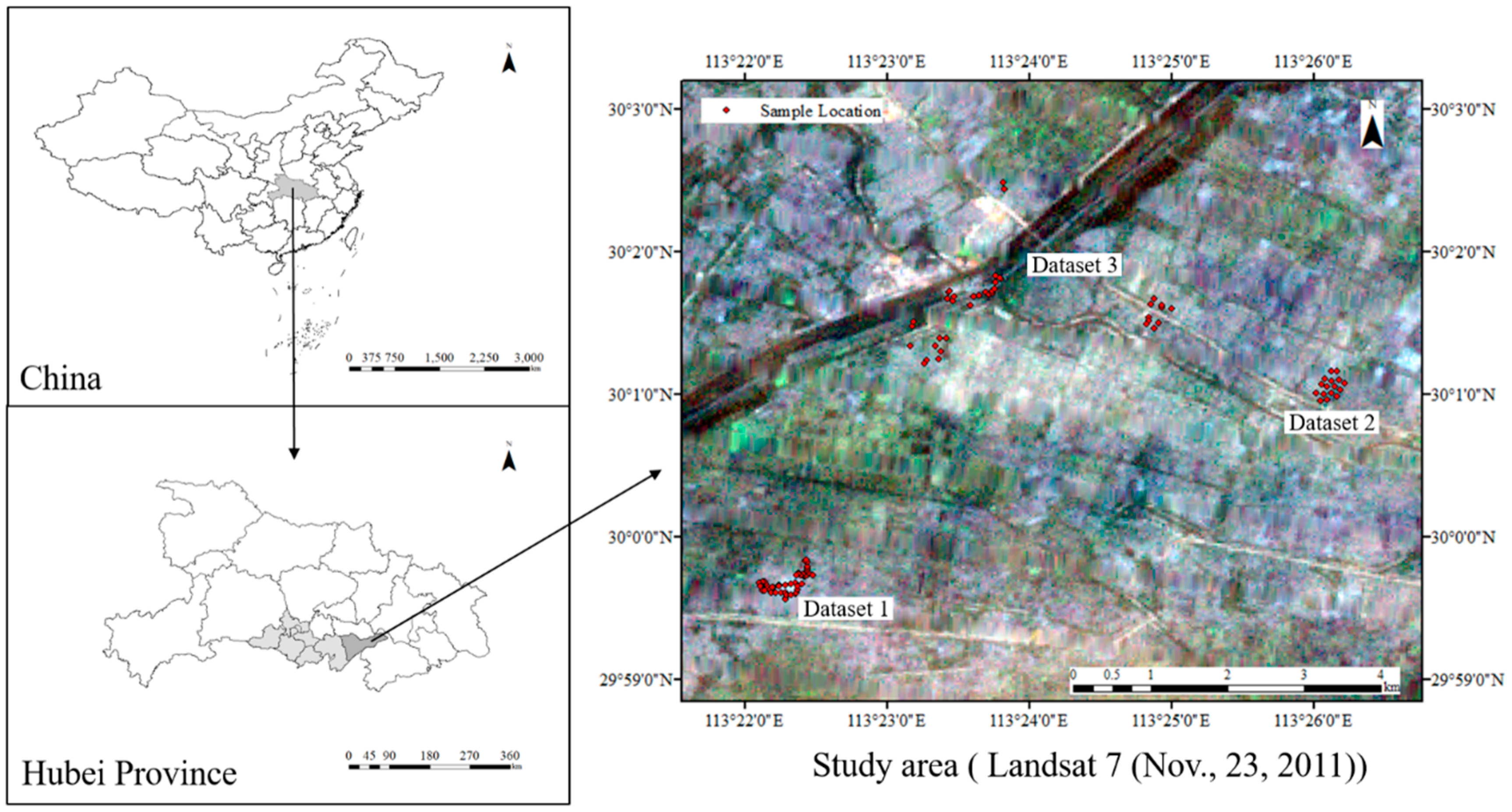
2.1. Sampling Area and Soil Samples
2.2. VIS-NIR Spectral Measurement and SOC Analysis
2.3. Spectral Pretreatment
2.4. Spectral Variable Selection
2.5. Model Calibration and Validation
3. Results
3.1. Statistical Description of Soil Samples
3.2. Raw Spectra and Pretreated Spectra
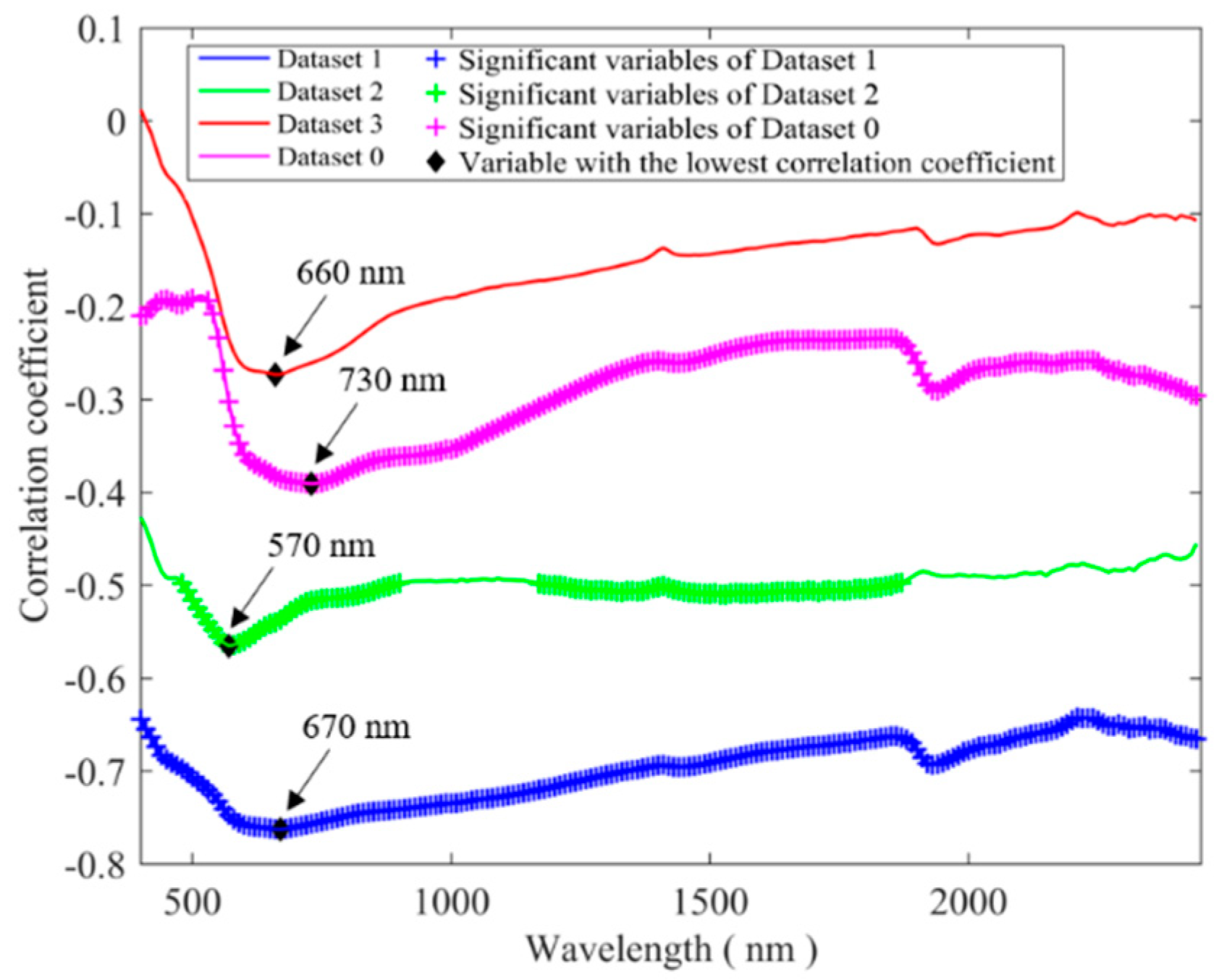
3.3. Correlation Analysis
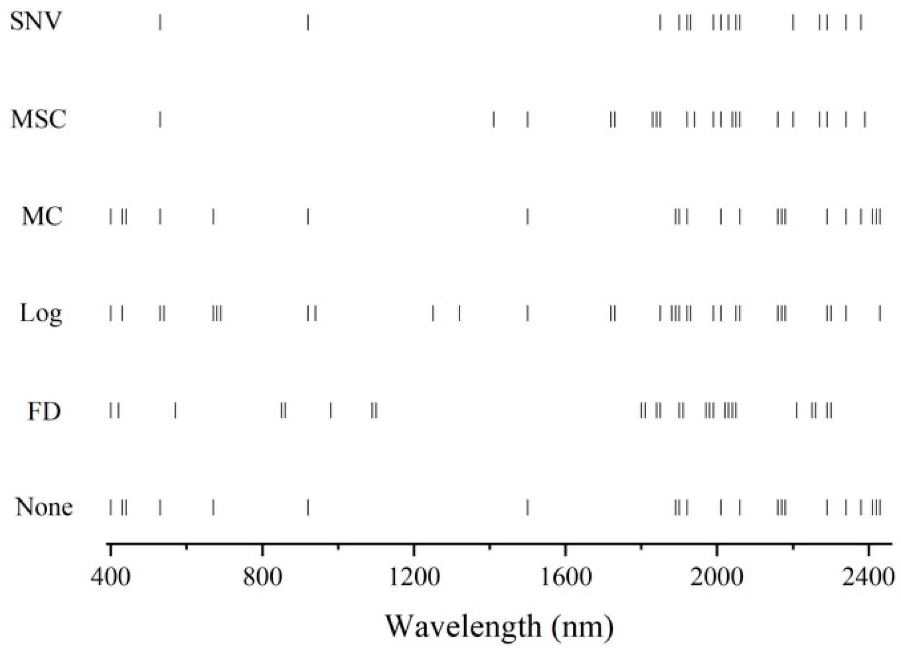
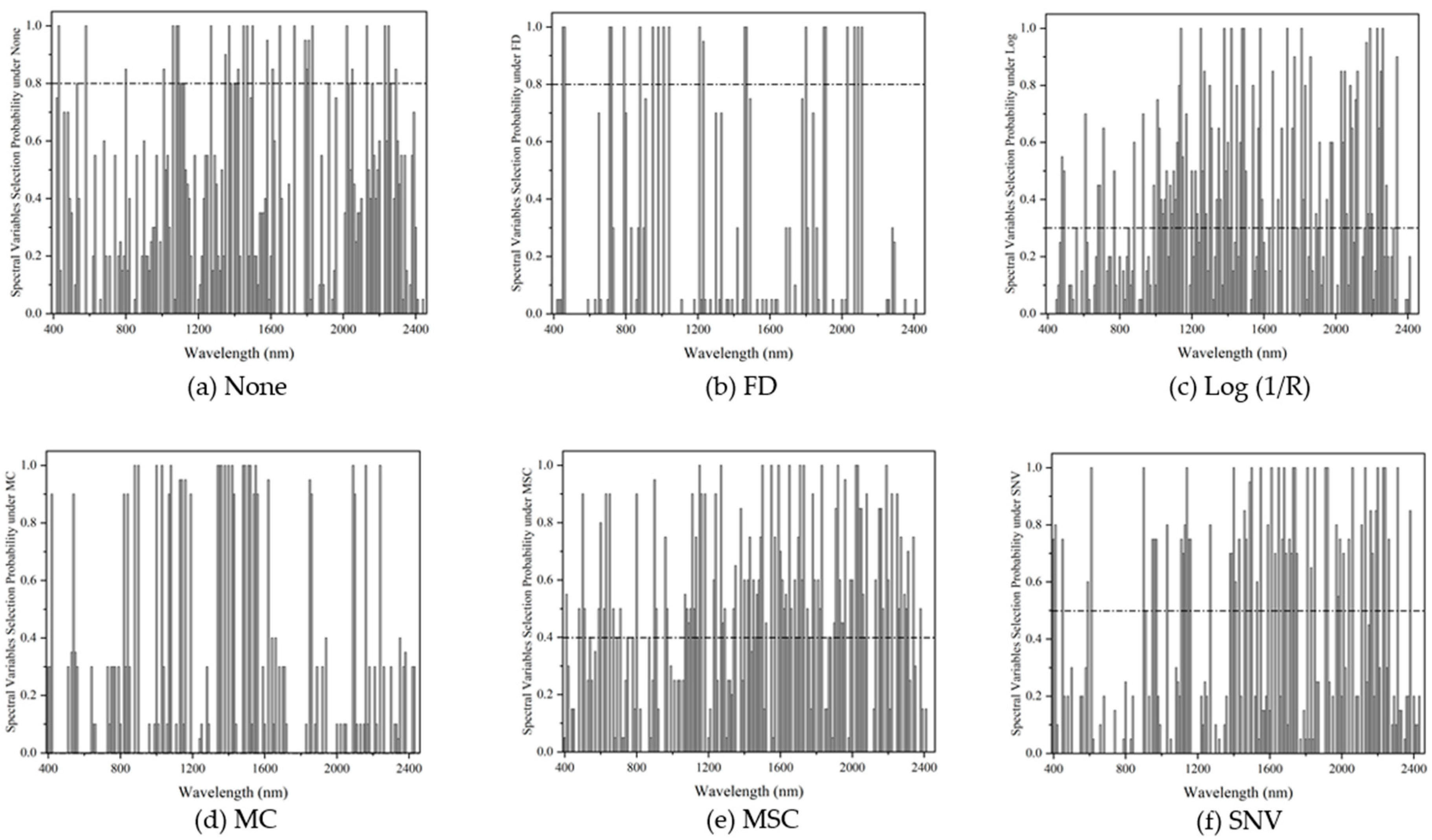
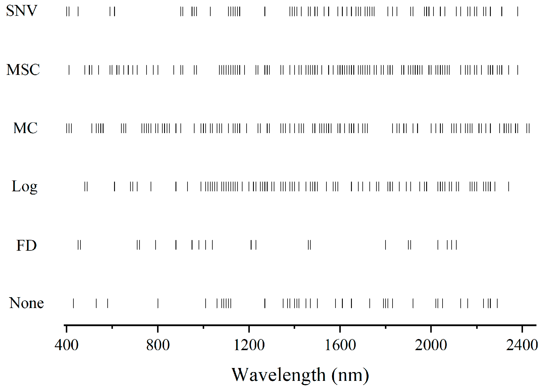
3.4. Spectral Variable Selection
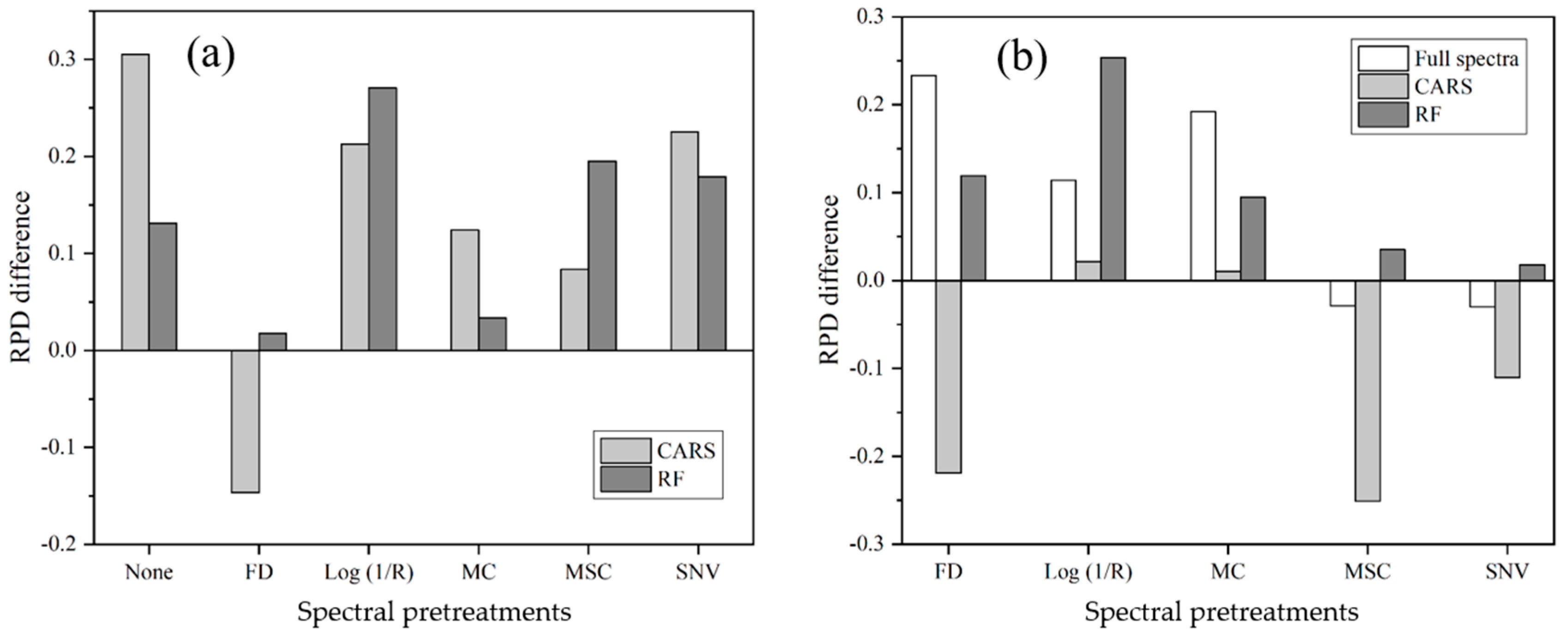
3.5. Accuracy of Estimation after Different Pretreatment and Variable Selection Techniques
4. Discussion
4.1. The Effect of Spectral Variable Selection Techniques on Model Accuracy
4.2. The Effect of Spectral Variable Selection Techniques on Model Parsimony
4.3. The Implication of the Proposed Strategy
5. Conclusions
Author Contributions
Funding
Acknowledgments
Conflicts of Interest
References
- Schmidt, M.W.; Torn, M.S.; Abiven, S.; Dittmar, T.; Guggenberger, G.; Janssens, I.A.; Kleber, M.; Kögel-Knabner, I.; Lehmann, J.; Manning, D.A.C.; et al. Persistence of Soil Organic Matter as an Ecosystem Property. Nat. Cell Biol. 2011, 478, 49–56. [Google Scholar] [CrossRef] [Green Version]
- Wiesmeier, M.; Urbanski, L.; Hobley, E.; Lang, B.; Von Lützow, M.; Marin-Spiotta, E.; Van Wesemael, B.; Rabot, E.; Ließ, M.; Garcia-Franco, N.; et al. Soil Organic Carbon Storage as a Key Function of Soils—A Review of Drivers and Indicators at Various Scales. Geoderma 2019, 333, 149–162. [Google Scholar] [CrossRef]
- Meuser, H. Anthropogenic Soils. In Contaminated Urban Soils; Meuser, H., Ed.; Springer: Dordrecht, The Netherlands, 2010; pp. 121–193. [Google Scholar]
- Dazzi, C.; Papa, G.L. Anthropogenic Soils: General Aspects and Features. Ecocycles 2015, 1, 3–8. [Google Scholar] [CrossRef] [Green Version]
- Davidson, E.; Trumbore, S.E.; Amundson, R. Soil Warming and Organic Carbon Content. Nat. Cell Biol. 2000, 408, 789–790. [Google Scholar] [CrossRef]
- Gholizadeh, A.; Saberioon, M.; Viscarra Rossel, R.A.; Boruvka, L.; Klement, A. Spectroscopic Measurements and Imaging of Soil Colour for Field Scale Estimation of Soil Organic Carbon. Geoderma 2020, 357, 113972. [Google Scholar] [CrossRef]
- Piao, S.; Fang, J.; Ciais, P.; Peylin, P.; Huang, Y.; Sitch, S.; Wang, T. The Carbon Balance of Terrestrial Ecosystems in China. Nat. Cell Biol. 2009, 458, 1009–1013. [Google Scholar] [CrossRef] [PubMed]
- Castaldi, F.; Chabrillat, S.; Chartin, C.; Genot, V.; Jones, A.; Van Wesemael, B. Estimation of Soil Organic Carbon in Arable Soil in Belgium and Luxembourg with the LUCAS Topsoil Database. Eur. J. Soil Sci. 2018, 69, 592–603. [Google Scholar] [CrossRef]
- Grover, S.; Butterly, C.R.; Wang, X.; Gleeson, D.B.; Macdonald, L.M.; Hall, D.; Tang, C. An Agricultural Practise with Climate and Food Security Benefits: “Claying” with Kaolinitic Clay Subsoil Decreased Soil Carbon Priming and Mineralisation in Sandy Cropping Soils. Sci. Total. Environ. 2020, 709, 134488. [Google Scholar] [CrossRef]
- McKenzie, N.; Cresswell, H.P.; Ryan, P.J.; Grundy, M.J. Contemporary Land Resource Survey Requires Improvements in Direct Soil Measurement. Commun. Soil Sci. Plant. Anal. 2000, 31, 1553–1569. [Google Scholar] [CrossRef]
- Shepherd, K.D.; Walsh, M.G. Development of Reflectance Spectral Libraries for Characterization of Soil Properties. Soil Sci. Soc. Am. J. 2002, 66, 988–998. [Google Scholar] [CrossRef]
- Ben-Dor, E.; Banin, A. Near-Infrared Analysis as a Rapid Method to Simultaneously Evaluate Several Soil Properties. Soil Sci. Soc. Am. J. 1995, 59, 364–372. [Google Scholar] [CrossRef]
- Chang, C.-W.; Laird, D.A. Near-Infrared Reflectance Spectroscopic Analysis of Soil C and N. Soil Sci. 2002, 167, 110–116. [Google Scholar] [CrossRef]
- Morra, M.J.; Hall, M.H.; Freeborn, L.L. Carbon and Nitrogen Analysis of Soil Fractions Using Near-Infrared Reflectance Spectroscopy. Soil Sci. Soc. Am. J. 1991, 55, 288–291. [Google Scholar] [CrossRef]
- Angelopoulou, T.; Tziolas, N.; Balafoutis, A.; Zalidis, G.; Bochtis, D. Remote Sensing Techniques for Soil Organic Carbon Estimation: A Review. Remote Sens. 2019, 11, 676. [Google Scholar] [CrossRef] [Green Version]
- Hong, Y.; Chen, Y.; Yu, L.; Liu, Y.; Liu, Y.; Zhang, Y.; Liu, Y.; Cheng, H. Combining Fractional Order Derivative and Spectral Variable Selection for Organic Matter Estimation of Homogeneous Soil Samples by VIS–NIR Spectroscopy. Remote Sens. 2018, 10, 479. [Google Scholar] [CrossRef] [Green Version]
- Kühnel, A.; Bogner, C. In-Situ Prediction of Soil Organic Carbon by Vis-NIR Spectroscopy: An Efficient Use of Limited Field Data. Eur. J. Soil Sci. 2017, 68, 689–702. [Google Scholar] [CrossRef]
- Liu, Y.; Jiang, Q.; Fei, T.; Wang, J.; Shi, T.; Guo, K.; Li, X.; Chen, Y. Transferability of a Visible and Near-Infrared Model for Soil Organic Matter Estimation in Riparian Landscapes. Remote Sens. 2014, 6, 4305–4322. [Google Scholar] [CrossRef] [Green Version]
- Garrity, D.; Bindraban, P. A Globally Distributed Soil Spectral Library, Visible Near Infrared Diffuse Reflectance Spectra; The ICRAF/ISRIC Spectral Library; Soil-Plant Spectral Diagnostics Laboratory: Nairobi, Kenya, 2004. [Google Scholar]
- Orgiazzi, A.; Ballabio, C.; Panagos, P.; Jones, A.; Fernández-Ugalde, O. LUCAS Soil, the Largest Expandable Soil Dataset for Europe: A Review. Eur. J. Soil Sci. 2017, 69, 140–153. [Google Scholar] [CrossRef] [Green Version]
- Demattê, J.A.; Dotto, A.C.; Paiva, A.F.; Sato, M.V.; Dalmolin, R.S.; De Araújo, M.D.S.B.; Da Silva, E.B.; Nanni, M.R.; Caten, A.T.; Noronha, N.C.; et al. The Brazilian Soil Spectral Library (BSSL): A General View, Application and Challenges. Geoderma 2019, 354, 113793. [Google Scholar] [CrossRef]
- Viscarra Rossel, R.A.; Webster, R. Predicting Soil Properties from the Australian Soil Visible-Near Infrared Spectroscopic Database. Eur. J. Soil Sci. 2012, 63, 848–860. [Google Scholar] [CrossRef]
- Shi, Z.; Wang, Q.; Peng, J.; Ji, W.; Liu, H.; Li, X.; Viscarra Rossel, R.A. Development of a National VNIR Soil-Spectral Library for Soil Classification and Prediction of Organic Matter Concentrations. Sci. China Earth Sci. 2014, 57, 1671–1680. [Google Scholar] [CrossRef]
- Stevens, A.; Nocita, M.; Tóth, G.; Montanarella, L.; Van Wesemael, B. Prediction of Soil Organic Carbon at the European Scale by Visible and Near InfraRed Reflectance Spectroscopy. PLoS ONE 2013, 8, e66409. [Google Scholar] [CrossRef] [PubMed]
- Guerrero, C.; Wetterlind, J.; Stenberg, B.; Mouazen, A.M.; Gabarrón-Galeote, M.A.; Ruiz-Sinoga, J.D.; Zornoza, R.; Viscarra Rossel, R.A. Do We Really Need Large Spectral Libraries for Local Scale SOC Assessment with NIR Spectroscopy? Soil Tillage Res. 2016, 155, 501–509. [Google Scholar] [CrossRef]
- Jin, X.; Du, J.; Liu, H.; Wang, Z.; Song, K. Remote Estimation of Soil Organic Matter Content in the Sanjiang Plain, Northest China: The Optimal Band Algorithm Versus the GRA-ANN Model. Agric. Meteorol. 2016, 218, 250–260. [Google Scholar] [CrossRef]
- Wetterlind, J.; Stenberg, B.; Söderström, M. Increased Sample Point Density in Farm Soil Mapping by Local Calibration of Visible and Near Infrared Prediction Models. Geoderma 2010, 156, 152–160. [Google Scholar] [CrossRef] [Green Version]
- Wetterlind, J.; Stenberg, B.; Söderström, M. Farm-Soil Mapping Using NIR-Technique for Increased Sample Point Density. In Precision Agriculture 2007—Papers Presented at the 6th European Conference on Precision Agriculture; Evangelical Christian Publishers Association (ECPA): Phoenix, AZ, USA, 2007; pp. 265–270. [Google Scholar]
- Stenberg, B.; Wetterlind, J. Small Sized Local vs. Large Sized National Calibration Sets and Their Combination for Farm Scale Predictions by NIR. In Geophysical Research Abstracts; European Geosciences Union: Munich, Germany, 2009. [Google Scholar]
- Wetterlind, J.; Stenberg, B.; Söderström, M. The Use of Near Infrared (NIR) Spectroscopy to Improve Soil Mapping at the Farm Scale. Precis. Agric. 2008, 9, 57–69. [Google Scholar] [CrossRef] [Green Version]
- Mehmood, T.; Liland, K.H.; Snipen, L.; Sæbø, S. A Review of Variable Selection Methods in Partial Least Squares Regression. Chemom. Intell. Lab. Syst. 2012, 118, 62–69. [Google Scholar] [CrossRef]
- Vohland, M.; Ludwig, M.; Thiele-Bruhn, S.; Ludwig, B. Quantification of Soil Properties with Hyperspectral Data: Selecting Spectral Variables with Different Methods to Improve Accuracies and Analyze Prediction Mechanisms. Remote Sens. 2017, 9, 1103. [Google Scholar] [CrossRef] [Green Version]
- Vohland, M.; Ludwig, M.; Harbich, M.; Emmerling, C.; Thiele-Bruhn, S. Using Variable Selection and Wavelets to Exploit the Full Potential of Visible–Near Infrared Spectra for Predicting Soil Properties. J. Near Infrared Spectrosc. 2016, 24, 255–269. [Google Scholar] [CrossRef]
- Chong, I.-G.; Jun, C.-H. Performance of Some Variable Selection Methods When Multicollinearity Is Present. Chemom. Intell. Lab. Syst. 2005, 78, 103–112. [Google Scholar] [CrossRef]
- Jia, S.; Li, H.; Wang, Y.; Tong, R.; Li, Q. Recursive Variable Selection to Update Near-Infrared Spectroscopy Model for the Determination of Soil Nitrogen and Organic Carbon. Geoderma 2016, 268, 92–99. [Google Scholar] [CrossRef]
- Galvão, R.K.H.; Araujo, M.C.U.; Fragoso, W.D.; Da Silva, E.C.; José, G.E.; Soares, S.F.C.; Paiva, H.M. A Variable Elimination Method to Improve the Parsimony of MLR Models Using the Successive Projections Algorithm. Chemom. Intell. Lab. Syst. 2008, 92, 83–91. [Google Scholar] [CrossRef]
- Li, H.; Liang, Y.-Z.; Xu, Q.; Cao, D. Key Wavelengths Screening Using Competitive Adaptive Reweighted Sampling Method for Multivariate Calibration. Anal. Chim. Acta 2009, 648, 77–84. [Google Scholar] [CrossRef] [PubMed]
- Leardi, R.; González, A.L. Genetic Algorithms Applied to Feature Selection in PLS Regression: How and When to Use Them. Chemom. Intell. Lab. Syst. 1998, 41, 195–207. [Google Scholar] [CrossRef]
- Kalivas, J.H.; Roberts, N.; Sutter, J.M. Global Optimization by Simulated Annealing with Wavelength Selection for Ultraviolet-Visible Spectrophotometry. Anal. Chem. 1989, 61, 2024–2030. [Google Scholar] [CrossRef]
- Li, H.-D.; Xu, Q.-S.; Liang, Y.-Z. Random Frog: An Efficient Reversible Jump Markov Chain Monte Carlo-Like Approach for Variable Selection with Applications to Gene Selection and Disease Classification. Anal. Chim. Acta 2012, 740, 20–26. [Google Scholar] [CrossRef]
- Zhang, Y.; Li, M.; Zheng, L.; Qin, Q.; Lee, W.S. Spectral Features Extraction for Estimation of Soil Total Nitrogen Content Based on Modified Ant Colony Optimization Algorithm. Geoderma 2019, 333, 23–34. [Google Scholar] [CrossRef]
- Vohland, M.; Ludwig, M.; Thiele-Bruhn, S.; Ludwig, B. Determination of Soil Properties with Visible to Near- and Mid-Infrared Spectroscopy: Effects of Spectral Variable Selection. Geoderma 2014, 223–225, 88–96. [Google Scholar] [CrossRef]
- Yao, X.; Yang, W.; Li, M.; Zhou, P.; Chen, Y.; Hao, Z.; Liu, Z. Prediction of Total Nitrogen in Soil Based on Random Frog Leaping Wavelet Neural Network. IFAC Pap. 2018, 51, 660–665. [Google Scholar] [CrossRef]
- Hu, M.; Dong, Q.; Liu, B.-L.; Opara, U.L.; Chen, L. Estimating Blueberry Mechanical Properties Based on Random Frog Selected Hyperspectral Data. Postharvest Biol. Technol. 2015, 106, 1–10. [Google Scholar] [CrossRef]
- Li, X.; Sun, C.; Luo, L.; He, Y. Determination of Tea Polyphenols Content by Infrared Spectroscopy Coupled with IPLS and Random Frog Techniques. Comput. Electron. Agric. 2015, 112, 28–35. [Google Scholar] [CrossRef]
- Gholizadeh, A.; Borůvka, L.; Saberioon, M.; Kozák, J.; Vašát, R.; Němeček, K. Comparing Different Data Preprocessing Methods for Monitoring Soil Heavy Metals Based on Soil Spectral Features. Soil Water Res. 2016, 10, 218–227. [Google Scholar] [CrossRef] [Green Version]
- Vašát, R.; Kodešová, R.; Klement, A.; Borůvka, L. Simple but Efficient Signal Pre-Processing in Soil Organic Carbon Spectroscopic Estimation. Geoderma 2017, 298, 46–53. [Google Scholar] [CrossRef]
- Gholizadeh, A.; Carmon, N.; Klement, A.; Ben-Dor, E.; Boruvka, L. Agricultural Soil Spectral Response and Properties Assessment: Effects of Measurement Protocol and Data Mining Technique. Remote Sens. 2017, 9, 1078. [Google Scholar] [CrossRef] [Green Version]
- Rinnan, Å.; Berg, F.V.D.; Engelsen, S.B. Review of the Most Common Pre-Processing Techniques for Near-Infrared Spectra. Trac Trends Anal. Chem. 2009, 28, 1201–1222. [Google Scholar] [CrossRef]
- Gholizadeh, A.; Žižala, D.; Saberioon, M.; Borůvka, L. Soil Organic Carbon and Texture Retrieving and Mapping Using Proximal, Airborne and Sentinel-2 Spectral Imaging. Remote Sens. Environ. 2018, 218, 89–103. [Google Scholar] [CrossRef]
- Echambadi, R.; Hess, J.D. Mean-Centering Does Not Alleviate Collinearity Problems in Moderated Multiple Regression Models. Mark. Sci. 2007, 26, 438–445. [Google Scholar] [CrossRef]
- Wu, Z.; Wang, B.; Huang, J.; An, Z.; Jiang, P.; Chen, Y.; Liu, Y. Estimating Soil Organic Carbon Density in Plains Using Landscape Metric-Based Regression Kriging Model. Soil Tillage Res. 2019, 195, 104381. [Google Scholar] [CrossRef]
- Shi, T.; Chen, Y.; Liu, H.; Wang, J.; Wu, G. Soil Organic Carbon Content Estimation with Laboratory-Based Visible–Near-Infrared Reflectance Spectroscopy: Feature Selection. Appl. Spectrosc. 2014, 68, 831–837. [Google Scholar] [CrossRef]
- Rossel, R.V.; Behrens, T. Using Data Mining to Model and Interpret Soil Diffuse Reflectance Spectra. Geoderma 2010, 158, 46–54. [Google Scholar] [CrossRef]
- Shi, Z.; Ji, W.; Viscarra Rossel, R.A.; Chen, S.; Zhou, Y. Prediction of Soil Organic Matter Using a Spatially Constrained Local Partial Least Squares Regression and the Chinese Vis-NIR Spectral Library. Eur. J. Soil Sci. 2015, 66, 679–687. [Google Scholar] [CrossRef]
- Pansu, M.; Gautheyrou, J. Handbook of Soil Analysis: Mineralogical Organic and Inorganic Methods; Springer: Berlin/Heidelberg, Germany, 2006. [Google Scholar]
- Wold, S.; Martens, H.; Wold, H. The Multivariate Calibration Problem in Chemistry Solved by the PLS Method; Springer: Berlin/Heidelberg, Germany, 1983; pp. 286–293. [Google Scholar]
- Li, S.; Ji, W.; Chen, S.; Peng, J.; Zhou, Y.; Shi, Z. Potential of VIS-NIR-SWIR Spectroscopy from the Chinese Soil Spectral Library for Assessment of Nitrogen Fertilization Rates in the Paddy-Rice Region, China. Remote Sens. 2015, 7, 7029–7043. [Google Scholar] [CrossRef] [Green Version]
- Liu, Y.; Liu, Y.; Chen, Y.; Zhang, Y.; Shi, T.; Wu, G.; Hong, Y.; Fei, T. The Influence of Spectral Pretreatment on the Selection of Representative Calibration Samples for Soil Organic Matter Estimation Using Vis-NIR Reflectance Spectroscopy. Remote Sens. 2019, 11, 450. [Google Scholar] [CrossRef] [Green Version]
- Cai, S.; Xia, X. The Wetland Resource of the Sihu Area and Its Exploitation. J. Resour. Environ. Yangtze Val. 1993, 2, 137–141. [Google Scholar]
- Wang, X.; Chen, Y.; Guo, L.; Liu, L. Construction of the Calibration Set through Multivariate Analysis in Visible and Near-Infrared Prediction Model for Estimating Soil Organic Matter. Remote Sens. 2017, 9, 201. [Google Scholar] [CrossRef] [Green Version]
- Liu, Y.; Chen, Y. Estimation of Total Iron Content in Floodplain Soils Using VNIR Spectroscopy—A Case Study in the Le’an River Floodplain, China. Int. J. Remote Sens. 2012, 33, 5954–5972. [Google Scholar] [CrossRef]
- Viscarra Rossel, R.A.; Minasny, B.; Roudier, P.; McBratney, A.B. Colour Space Models for Soil Science. Geoderma 2006, 133, 320–337. [Google Scholar] [CrossRef]
- Lacerda, M.P.C.; Demattê, J.A.; Sato, M.V.; Fongaro, C.T.; Gallo, B.; Souza, A.B. Tropical Texture Determination by Proximal Sensing Using a Regional Spectral Library and Its Relationship with Soil Classification. Remote Sens. 2016, 8, 701. [Google Scholar] [CrossRef] [Green Version]
- Ladoni, M.; Bahrami, H.A.; Alavipanah, S.K.; Noroozi, A.A. Estimating Soil Organic Carbon from Soil Reflectance: A Review. Precis. Agric. 2009, 11, 82–99. [Google Scholar] [CrossRef]
- Stenberg, B.; Viscarra Rossel, R.A.; Mouazen, A.M.; Wetterlind, J. Visible and Near Infrared Spectroscopy in Soil Science. In Advances in Agronomy; Academic Press: Cambridge, MA, USA, 2010; Volume 107, pp. 163–215. [Google Scholar]


| Samples | N a | SOC (g/kg) | SD d | CV e | CS f | CK g | ||
|---|---|---|---|---|---|---|---|---|
| Min b | Max c | Mean | ||||||
| Total | 103 | 2.35 | 33.95 | 16.05 | 6.35 | 40% | −0.04 | 2.32 |
| Calibration | 69 | 2.35 | 33.95 | 16.14 | 6.46 | 40% | 0.04 | 2.46 |
| Validation | 34 | 3.30 | 26.23 | 15.85 | 6.20 | 39% | −0.23 | 1.93 |
| Spectral Variable Selection | Spectral Pretreatments | N a | LVs b | Calibration Dataset | Validation Dataset | RPD | |||
|---|---|---|---|---|---|---|---|---|---|
| Rc2 | RMSEc | Rp2 | RMSEp | ||||||
| Full Spectra | None | 205 | 9 | 0.79 | 2.93 | 0.70 | 3.60 | 1.72 | 1.81 |
| FD | 205 | 7 | 0.78 | 3.01 | 0.80 | 3.17 | 1.96 | ||
| Log(1/R) | 205 | 11 | 0.86 | 2.44 | 0.76 | 3.37 | 1.84 | ||
| MC | 205 | 10 | 0.86 | 2.36 | 0.75 | 3.24 | 1.92 | ||
| MSC | 205 | 8 | 0.78 | 3.02 | 0.70 | 3.66 | 1.70 | ||
| SNV | 205 | 8 | 0.78 | 3.02 | 0.70 | 3.66 | 1.69 | ||
| CARS | None | 21 | 8 | 0.85 | 2.45 | 0.78 | 3.05 | 2.03 | 1.94 |
| FD | 26 | 7 | 0.85 | 2.44 | 0.73 | 3.42 | 1.81 | ||
| Log(1/R) | 31 | 8 | 0.84 | 2.53 | 0.81 | 3.02 | 2.05 | ||
| MC | 21 | 8 | 0.87 | 2.35 | 0.78 | 3.04 | 2.04 | ||
| MSC | 21 | 6 | 0.79 | 2.91 | 0.77 | 3.49 | 1.78 | ||
| SNV | 16 | 6 | 0.83 | 2.66 | 0.77 | 3.23 | 1.92 | ||
| RF | None | 39 | 10 | 0.83 | 2.61 | 0.72 | 3.34 | 1.86 | 1.94 |
| FD | 21 | 14 | 0.84 | 2.53 | 0.76 | 3.14 | 1.97 | ||
| Log(1/R) | 83 | 11 | 0.86 | 2.42 | 0.83 | 2.94 | 2.11 | ||
| MC | 101 | 10 | 0.85 | 2.45 | 0.77 | 3.18 | 1.95 | ||
| MSC | 106 | 11 | 0.89 | 2.16 | 0.76 | 3.28 | 1.89 | ||
| SNV | 63 | 8 | 0.81 | 2.83 | 0.77 | 3.31 | 1.87 | ||
| Locations of Selected Spectral Variables (nm) | Possible Fundamental Bonds | Possible Wavelength (nm) | Possible Related Soil Constituents |
|---|---|---|---|
| 800 | C–H | 825 | Organics (aromatics) |
| 1000 | N–H | 1000 | Organics (amine) |
| 1100 | C–H | 1100 | Organics (aromatics) |
| 1200 | C–H | 1170 | Organics (Alkyl asymmetric-symmetric doublet) |
| 1420 | O–H | 1380 | Water |
| 1500 | C–O | 1524 | Organics (amides) |
| 1800 | C–H | 1754 | Organics (Alkyl asymmetric-symmetric doublet) |
| 1920 | O–H | 1915 | Water |
| 2000 | C–O | 2033 | Organics (amides) |
| 2100 | N–H | 2060 | Organics (amine) |
| 2200 | Al–OH | 2230 | Clay minerals |
| 2350 | C–O | 2381 | Organics (Carbohydrates) |
Publisher’s Note: MDPI stays neutral with regard to jurisdictional claims in published maps and institutional affiliations. |
© 2020 by the authors. Licensee MDPI, Basel, Switzerland. This article is an open access article distributed under the terms and conditions of the Creative Commons Attribution (CC BY) license (http://creativecommons.org/licenses/by/4.0/).
Share and Cite
Xu, L.; Hong, Y.; Wei, Y.; Guo, L.; Shi, T.; Liu, Y.; Jiang, Q.; Fei, T.; Liu, Y.; Mouazen, A.M.; et al. Estimation of Organic Carbon in Anthropogenic Soil by VIS-NIR Spectroscopy: Effect of Variable Selection. Remote Sens. 2020, 12, 3394. https://doi.org/10.3390/rs12203394
Xu L, Hong Y, Wei Y, Guo L, Shi T, Liu Y, Jiang Q, Fei T, Liu Y, Mouazen AM, et al. Estimation of Organic Carbon in Anthropogenic Soil by VIS-NIR Spectroscopy: Effect of Variable Selection. Remote Sensing. 2020; 12(20):3394. https://doi.org/10.3390/rs12203394
Chicago/Turabian StyleXu, Lu, Yongsheng Hong, Yu Wei, Long Guo, Tiezhu Shi, Yi Liu, Qinghu Jiang, Teng Fei, Yaolin Liu, Abdul M. Mouazen, and et al. 2020. "Estimation of Organic Carbon in Anthropogenic Soil by VIS-NIR Spectroscopy: Effect of Variable Selection" Remote Sensing 12, no. 20: 3394. https://doi.org/10.3390/rs12203394
APA StyleXu, L., Hong, Y., Wei, Y., Guo, L., Shi, T., Liu, Y., Jiang, Q., Fei, T., Liu, Y., Mouazen, A. M., & Chen, Y. (2020). Estimation of Organic Carbon in Anthropogenic Soil by VIS-NIR Spectroscopy: Effect of Variable Selection. Remote Sensing, 12(20), 3394. https://doi.org/10.3390/rs12203394