Abstract
Urban heat islands (UHIs) can present significant risks to human health. Santiago, Chile has around 7 million residents, concentrated in an average density of 480 people/km2. During the last few summer seasons, the highest extreme maximum temperatures in over 100 years have been recorded. Given the projections in temperature increase for this metropolitan region over the next 50 years, the Santiago UHI could have an important impact on the health and stress of the general population. We studied the presence and spatial variability of UHIs in Santiago during the summer seasons from 2005 to 2017 using Moderate Resolution Imaging Spectroradiometer (MODIS) satellite imagery and data from nine meteorological stations. Simple regression models, geographic weighted regression (GWR) models and geostatistical interpolations were used to find nocturnal thermal differences in UHIs of up to 9 °C, as well as increases in the magnitude and extension of the daytime heat island from summer 2014 to 2017. Understanding the behavior of the UHI of Santiago, Chile, is important for urban planners and local decision makers. Additionally, understanding the spatial pattern of the UHI could improve knowledge about how urban areas experience and could mitigate climate change.
1. Introduction
Recent climate change studies evidence an increase in the intensity of extreme heat temperatures [1]. At the same time, on a global scale, rapid urban population growth is taking place [2,3], which combined with high temperatures, significantly increases health risks for the majority of the population. Hence, there is an increased mortality rate due to heat stress, which contributes to night-time insomnia, and causes respiratory illnesses produced by ozone (O3) [4]. All these factors can negatively impact work productivity and urban metabolism [5]. These processes consider the exchange of matter, energy and information established between an urban settlement and its natural environment. In this manner, the city is considered a living organism, incorporating measurements of technical and socio-economic processes that result from resource consumption, growth, energy production, and waste management [6,7].
The temperature distribution is not homogeneous over the landscape; the urban areas tend to have higher air temperature than their rural surrounding, a phenomenon known as urban heat island (UHI), the UHI is mainly caused by the anthropogenic land surface modifications, e.g. urban areas present higher heat concentration given that buildings absorb, retain and produce heat [8]. This temperature increase is influenced by the fact that an important number of human activities provoke alterations in the energy balance due to land use modification, surface properties (roughness, albedo, emissivity), and the geometry of the urban area [9]. In addition, air conditioning and heating systems of buildings, as well as traffic, are considered some of the biggest promoters of environmental warming in the city [10]. Other non-anthropogenic factors that can also affect the behavior of the UHI are the local vegetation cover and properties, seasonal variability of the weather, specific geographic characteristics of city locations, the presence of water bodies or wetlands, and even climate change, among others [11].
There are two types of UHI, the first one is the atmospheric urban heat island (UHI), that is defined as the difference between the air temperature (AT) within the city and the AT of its surroundings, measure 1–2 m above ground. The second is the surface urban heat island (SUHI) which is the study of the land surface temperature (LST), as opposed to the AT, that shows different temperatures on artificial and natural surfaces in the urban area [12], and that is usually measured using remote-sensing data [13], presenting different magnitudes than the UHI [10]. Various methods exist for using satellite methods for studying UHI by estimating air temperatures. Some examples of studies that have used this method have been carried out in Paris [14], Valencia [10], El Cairo [8], Singapore [15], West Midlands [16] and Bangkok [17], among others.
Multiple studies demonstrate temperature variations between urban and rural areas, as well as the satellite capacity to study these phenomena [18,19]. Several satellite products consider thermal bands within their design [20], and these include: Advanced Spaceborne Thermal Emission and Reflection (ASTER), Landsat Thermal Mapper (TM)/ Enhanced Thermal Mapper Plus (ETM+) [21,22], Geostationary Operation Environmental Satellite Program (GOES), Advance Very High Resolution Radiometer (AVHRR) or Moderate Resolution Imaging Spectroradiometer (MODIS LST) [23,24,25]. The first three have a high spatial resolution but low temporal resolution, and the last three have a high temporal resolution but low spatial resolution.
To study UHIs, it is crucial to have images of high periodicity more than those with a high spatial resolution [26]. Hence, for this study, we decided to use images from MODIS LST (MOD11A1 V6) because they have daily periodicity on two platforms (TERRA and AQUA), allowing us to obtain daytime and night-time imagery, and at the same time, the current product version has advantages due to its updated algorithm and quality control compared to previous versions [27]. MODIS data is widely used to characterize the UHI [11], Examples of this are [18], where the UHI was assessed in Nanjing, China, using LST, NDVI, and albedo products from MODIS, and [26], where MODIS was used to quantify the magnitude of the Birmingham surface UHI as well as the impact of atmospheric stability on UHI development. The MODIS products allow for the study of thermal variations throughout the UHI, as well as variations over time. Furthermore, these products enable the study of UHI at night during summer seasons, which is when it reaches its highest magnitudes [10].
Heatwaves present serious health risks for humans, and some authors place them among the biggest problems of the XXI century [28]. In the past few years, Santiago, Chile has registered the highest extreme maximum temperatures in over 100 years [29]. Likewise, in the Metropolitan Region of Santiago, there are around 7 million residents with a population density of 480 people/km2 [30]. Therefore, it is important to understand temperature differences and UHIs in the region and their spatial distribution and behavior over time with regards to geographic extension and movement, as well as their temperature magnitudes. The effects on mortality due to high temperatures in Santiago were studied by [31], leading to the conclusion that higher temperatures could be related to increased mortality risks, especially for the elderly population. Additionally, [32] concluded that, for Santiago, heat effects have an immediate impact on the mortality of the city‘s population.
In the same city, studies have researched urban heat sinks using Landsat ETM+ data [33], and urban heat islands using a limited amount of MODIS data (53 images) to make a seasonal characterization of the phenomena using Principal Component Analysis [25].
For this study, we evaluated the presence and spatio-temporal variability of UHIs of Santiago, Chile in summer periods from 2005 to 2017 using a dense time-series of satellite data to perform a detailed characterization of the phenomenon. To carry out this study, we used MODIS satellite images and data from nine weather stations belonging to the Chilean Ministry of Environment (MMA in Spanish).
We defined two main objectives for our study:
- Determination of the relationship between air temperature and satellite-derived LST.
- Analysis of historical UHI spatio-temporal temperature behavior.
2. Materials
2.1. Study Area
The Metropolitan Region of Santiago, Chile is home to the nation’s capital and comprises 52 communes and six provinces. Approximately 40.5% of the country’s population lives within this region (7,036,792 residents) [34], representing a density of 456.86 inhabitants per square kilometer, (the highest in the country). This region is distributed in urban, semi-urban, and rural communes, and the rural areas become more expansive as the distance increases from the center of the region [30]. The native vegetation of the Metropolitan Region consists mainly of grasslands and shrublands, covering 28.24% of the surface of the region, with native Sclerophyllus (Mediterranean) forest covering 24.24% of the surface. Water bodies cover only 0.56% of the region (data retrieved from the official land use information used by the Forestry Service of Chile, CONAF) with the closest water body to Santiago being the Aculeo Lagoon, located more than 20 km south from the city. The city is surrounded by the Andes mountain range, which presents altitudes of over 5 km above sea level to the east, and a much smaller coastal mountain range to the west, which presents a maximum altitude of 1880 m above sea level.
Data were taken from nine weather stations, eight of which are found in the urban area and one in a rural area in Talagante (see Figure 1). Data were also taken from MODIS images covering the entire region.
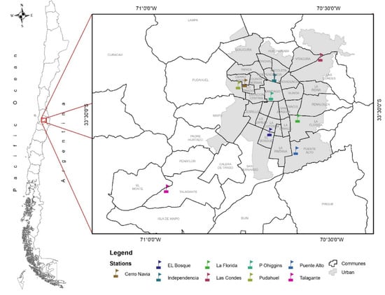
Figure 1.
Study area, administrative zones (communes), and location of the meteorological station, which are part of the National Information System of Air Quality (SINCA, by its initials in Spanish) in the city of Santiago, Chile.
2.2. Satellite Data
There are about 34 products generated by NASA that utilize information from data collected by the MODIS sensor in its TERRA and AQUA platforms. The product used in this study was the MOD11A1, with land surface temperatures obtained daily at 1 km of spatial resolution, presenting level 3 processing, version 6. Using MODIStsp R package tools [35], 1068 day and night images were downloaded and processed, corresponding to daily LSTs for the months of December, January, and February for the 12 years considered in this study (2005–2017).
Image acquisition time from the study area includes pixels with a difference of up to three daylight hours and three nighttime hours.
2.3. Meteorological Data
For land reference data, air temperatures from 2005 to 2017 were used from the nine weather stations belonging to the Chilean Ministry of the Environment and distributed in nine communes within the region, with the same date range as the satellite images, according to their availability (Table 1).

Table 1.
Meteorological stations (Ministry of Environment) record 2005–2017.
From hourly temperature data (24 daily registered temperatures), a database was created that allowed the verification of the spatio-temporal thermal variation between all nine weather stations. However, inconsistencies and extreme differences between stations (presumably due to a lack of maintenance or bad performance of the stations) made it necessary to conduct a revision (depuration) and validation in various stages. The Spanish regulation AENOR 500,540 was chosen, which, in accordance with [36], consists of seven types of successive validations of the weather data. These validations are numbered in levels from 0 (zero) to 6 (six); levels 0 and 1 are obligatory.
3. Methods
3.1. Spatially Explicit Model of the Daily Air Temperature (Day/Night)
To study UHIs, it is necessary to have periodic and spatially distributed temperature data. Integrating weather station data and satellite images allows for an adjustment of the statistical models, and hence the calibration of LST. Later, through models, this information can be extended to the total study area [37].
The MODIS sensor in MOD11A1 includes a view of the study area two times a day at three different times: in the morning onboard the TERRA Satellite at 9:00, 10:00, and 11:00 h; and at night on the AQUA platform at 22:00, 23:00, and 24:00 h local time. These satellite data are among of the dominant sources of remote-sensing images for investigating the UHI effect, due to its high temporal resolution [11]. All daily images and weather station data are paired according to date, time, and location in order to conform to the database used to analyze.
Figure 2 shows the methodological outline used to obtain the daily images for air temperature, using LST images and other precise data from the nine weather stations.
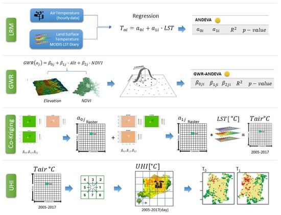
Figure 2.
The methodological scheme is divided into four steps: Step 1 is in regards to linear regression models (LRM) estimating air temperature from land surface temperature. After that, it is necessary to consider the estimation of LRM parameters considering their spatial position using geographic weighted models (Step 2). In Step 3, we use bivariate interpolation models as a cokriging to estimate the air temperature for each pixel of the area. Finally (Step 4), the urban heat island (UHI) is calculated for different dates, studying its behavior in all periods.
3.1.1. Linear Regression Model (LRM)
To understand the relationship between LST and the air temperature measured at each one of the stations, a linear model adjustment (Equation (1)) was carried out for the daytime, nighttime, and mixed satellite data with temperature data from each station. The nine resulting models were evaluated according to their determination coefficient (R2), standard error, statistical significance (p-value), and correlation coefficient (R).
where is the air temperature estimate in point ; is the intercept in point ; is the slope in point and is the model error.
As a result of this process, regardless of the data included in the models, an equation is obtained that allows determination of local air temperature using the LST pixel value registered by the satellite for the modeled station.
The exact condition of the adjusted models does not allow for the prediction of the air temperature for all pixels in the image, given that the pixel-station adjustment is only valid inside this. If extending the models to intermediate or neighboring pixels is to be considered, the presence of spatial autocorrelation in the temperature should be noted. The latter discards traditional statistical models because they do not comply with the requirement that the observations be independent [38].
To estimate the temperature in each image pixel, coefficients obtained from the nine linear models (local) were adjusted to values that take into account the special relationships between the data [39]. This is done assuming that the temperature does not randomly vary, but that the relationship between variables varies depending on the study area location [40].
3.1.2. Spatially Explicit Regression Models (GWR)
Geographically weighted regression (GWR) models are local models that create an equation for each element of the dependent variable dataset [40]. In this case, the coefficients (a0, a1) from the nine equations were modeled using two independent variables: the NDVI vegetation index and altitude, given their known relationship with temperature [41]. The general GWR model can be seen in Equation (2).
where (Ui, Vi) are the geographic coordinates of point i and is the value calculated from the continuous function in point i [42].
Geographic regression allows for the improvement of adjustments, neutralizing spatial dependency on residues, and understanding the special distribution of the elasticity of the explicative variables, as well as the model’s local significance [38].
Equation (3) shows the GWR model, where data for the altitude variable are obtained directly from the NASA product GTOPO 30 [43], with a spatial resolution of 30 arc seconds (approximately 1 km). Data from the NDVI are obtained from a personalized product through Google Earth Engine, which is a composition of the maximum values for each pixel from all of the available NDVI images during the study period, the implementation of the Landsat 8 sensor (2013–2017), and subsequent resampling at a 1-km resolution.
3.1.3. Cokriging of Coefficients
After adjusting the GWRs, a geostatistical interpolation model is employed that allows for the estimation of the coefficients of all pixels in the study area where weather stations do not exist. This interpolation model corresponds to ordinary cokriging, where variable means are unknown [44]. This can be seen in Equation (4).
where is the value measured at location i; is an unknown ponderation for the measured value at location i; is the prediction location and N is the number of values measured. In this way, the two spatialized coefficients () are obtained using Equation (3) from the spatialized coefficients, using Equation (4) for application in the linear model and Equation (1) for air temperature estimations.
3.2. Calculation and Analysis of UHIs
To calculate the heat island, we used the Talagante weather station as a reference, given that it is a rural area around Santiago. Complementarily, this selection was validated through cluster analysis on the spatialized air temperature coefficients (a0 and a1), and a zonal statistical calculation to a commune scale level using the mean maximum NDVI during the period of analysis. The NDVI presents a high inverse correlation with thermal emissivity [36,37], which demonstrates thermal differences between rural and urban areas if the former has a higher presence of vegetation.
Temperature at the Talagante station is subtracted from the modelled temperature in each pixel for each day and night. In this manner, the values represented in the UHI imagery correspond to the differences between temperatures in a rural area and an urban one. Finally, to improve spatio-temporal analysis, calculations were carried out based on the images of average, maximum UHI, and standard deviations on a monthly scale and during the summer seasons.
The fit integrity for each model was evaluated over the daily values (Table 2), through systematic error determination (BIAS), mean absolute error (MAE), root mean square error (RMSE), and the determination coefficient (R2). The agreement index (d) ([45,46,47,48,49]) and the Akaike information criterion (AIC) ([50,51]) were also calculated.
Table 2.
Statistical criteria used to evaluate model performance.
4. Results
4.1. Meteorological Database
The application of different data validation levels (AENOR 500540) was considered for each one of the nine stations. During the validation process, 4535 records were eliminated (2% of the total), which added to the 11,604 missing records (5.1% of the total). There were periods in which no data were registered at any station, principally between 15 December 2015 and 18 February 2016. All stations had periods in which no information was recorded for hours, or in some cases, days.
4.2. Spatially Explicit Model of the Daily Air Temperature (Day/Night)
Optimal results from the adjustment and evaluation of the daytime, nighttime, and mixed linear models were obtained from both daytime and nighttime joint data (mixed). There was a clear difference in the adjustment in the mixed models (R2 range 0.643–0.853), and therefore it was much better than daytime (R2 range 0.254–0.480) or nighttime (R2 range 0.172–0.358) as individual data sets.
For the mixed models, the coefficients of each adjustment are shown in Table 3. Regular values were obtained for the slope coefficient except for the Talagante station, because it had a completely different slope and intercept behavior. Since this station is located in a rural area, data from the Talagante station backed the decision to use it as a reference for calculating UHI.
Table 3.
Models and coefficients by the station.
Stations Puente Alto and Las Condes were closer in their coefficients, coinciding with the fact that, except for Talagante, they are the furthest stations away from the central urban nucleus, and both are found in the eastern sector of the city, in the foothills of the Andes Mountains (Figure 1).
Stations La Florida and El Bosque presented similar intercepts. Spatially, both stations are located in the south-western part of the city, close to the main arterial avenue Américo Vespucio.
Cerro Navia and Parque O’Higgins stations also had close intercepts, and both are located toward the city center. Furthermore, both stations are possibly affected by colder air entering through a corridor formed by the air approach path to the ex-airport Cerrillos, located in the same district [52].
Finally, Pudahuel and Independencia stations were the most northern and western stations, respectively, and both registered similar intercepts.
As a result of the geographically weighted regression (GWR) models, coefficients a0 and a1 were obtained and adjusted considering altitude and NDVI in the model (Equation (3)). Table 4 shows the a0 and a1 coefficient averages, their estimation error percentage, and general statistics for each model. The determination coefficients (R2) for both models were higher than 88%, presenting a low mean, standard error, and significance level of a p-value less than 0.001.
Table 4.
Results from geographically weighted regression (GWR) models.
To spatialize the new coefficients and obtain their values for each pixel of the study area, a geostatistical interpolation model was used. This allowed for spatial autocorrelation modeling of the variable though adjustment of the semi-variograms linked to each variable and any relationships among them. The chosen estimation model was an ordinary cokriging, modeling its variables with spherical models fitted through two-stage processes that optimized the adjustment [53]. The result of this process was a coefficient raster map for a0 and a1, completing in each pixel a linear equation that estimated air temperature using LST.
4.3. Calculation and Analysis of UHIs
To confirm the selection of the Talagante station as the rural reference, two independent analyses were carried out. The first was through the calculation of the average of all commune pixels with a maximum NDVI value, and the second through a K-means cluster analysis on coefficients from the linear models by pixel station (located on each meteorological stations). Both results validated that it was a rural zone (high average NDVI), and that it was statistically part of an independent group (Figure 3), allowing for temperature difference calculations for each pixel versus the reference pixel (UHI) for each day and each night of the period.
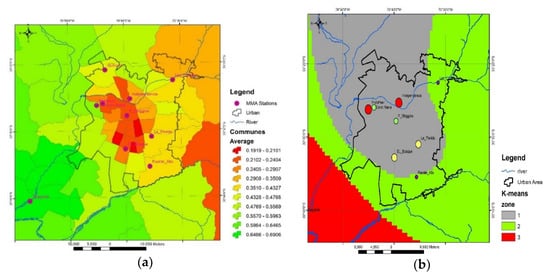
Figure 3.
Zonal average of maximum NDVI for each period and commune (a); K-means cluster analysis on coefficients calculated from the linear models by meteorological stations (b).
Average, maximums, and UHI dispersions were evaluated for each pixel during every summer day (December, January, and February) for all years of the study period. The highest median daytime temperatures in the heat island were concentrated in the northwest sector of Santiago (Figure 4). This island increases its extension toward the center of the city, covering almost half of the urban area during February. Regarding magnitude, magnitudes increase towards February, reaching 4 °C.
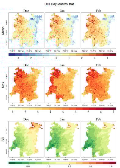
Figure 4.
Daytime urban heat islands (based on daily data from 2005 to 2017). UHI is calculated from the difference between the pixels and the rural station of reference (Talagante station). The first row shows the mean monthly temperatures of December, January, and February; the central row shows the average of the maximum temperature of the same period; the last row shows the average standard deviation of temperatures. Mean: Heat increases in intensity towards the northwest zones as February approaches, while also advancing to the center of the city. Max: The maximum temperature behavior in December and February are similar, but January has the maximum higher temperature towards the west zone. SD: The standard deviation increases from southwest to northeast; this trend continues from December to February, decreasing variability towards the end of summer.
Conversely, the average nighttime temperatures of the UHI presented similar extensions during all three summer months (Figure 5). The same was true for its magnitude, which reached 5 °C. The extension of the island covered the entire urban area, which was different to the daytime island in which temperatures were below reference levels in the foothills region, a phenomenon that can be caused by the cooling effect of the breezes coming from the Andes range [52].
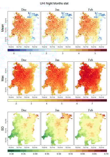
Figure 5.
Nocturnal urban heat island (based on data from 2005 to 2017). Nocturnal UHI is calculated using images at nocturnal acquisition times (22, 23, or 24 h). The first row shows the behavior the nocturnal mean monthly temperature of December, January, and February; the central row shows the maximum nocturnal temperature average of the same period; the last row shows the average standard deviation of the nocturnal temperature. Mean: The mean night temperature is regular in its extension and intensity throughout the period and study area. Max: The maximum night temperature’s behavior is similar during the three summer months, but the intensity is greatest in February. SD: The standard deviation night temperature increases mainly in January in the city center, and stays down near the rural station of reference during the whole summer.
The maximum daytime temperatures of the heat island concentrated their highest values towards the northwest sector of the urban area (Quilicura commune), which corresponds to one of the communes with the lowest percentage of green areas within Santiago [54]. During the entire season, except for during the maximum January temperatures, higher values were homogeneously distributed throughout the whole urban area. In January, maximum temperatures tended to concentrate toward the western limit, decreasing in magnitude in the central zone and foothills. The daytime maximums reached 9 °C, and there were no sectors less than 1 °C.
Maximum nocturnal temperatures of the heat island (Figure 5) were higher in magnitude and extension than daily temperatures, meaning that they covered the entire urban area with values higher than 2 °C, increasing intensity in February, up to 7.5 °C. Extreme nocturnal temperature values extended their concentration during February, moving toward the urban center over the sectors of stations Parque O’Higgin, Quilicura, Cerro Navia, and Independencia. The three latter stations are located in communes that present a relatively low percentage of green spaces compared to the rest of the city [54].
Regarding thermal dispersion of the heat island, a higher variation was observed in the northeast sector of the city during December using daytime data; this decreased as summer progressed. The most stable section (least dispersion) was in the southwest sector, where the influence of cooler air [52] maintains area stability. During the night, the heat island had a nucleus with a higher dispersion on the eastern limit of Santiago, in the commune of Providencia. In the northwest sector, in the commune of Ñuñoa, dispersion of nocturnal thermal variation monthly data increased mainly during the month of February.
Averages for the data on the daily and nocturnal UHI for each summer can be observed in Figure 6. These averages did not undergo significant variations between summers regarding the average monthly, daily, and nocturnal behavior (Figure 4 and Figure 5). On the other hand, the maximum daytime temperatures of the heat island had cyclical behavior (Figure 7), decreasing their values towards the summer of 2010–2011.
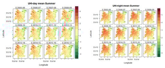
Figure 6.
Average daily and nocturnal UHI for the 2005–2017 summer seasons. Each summer season considers the month of December for the prior year and January and February of the following year (e.g., S 2005–2006 means December 2005 and January and February 2006). The graph shows the mean day and night temperatures over three months. The main difference is that during the night the UHI is more intense in temperature and extent. In the day, the UHI is high only in the northwest extending to the center, but ultimately loses intensity.
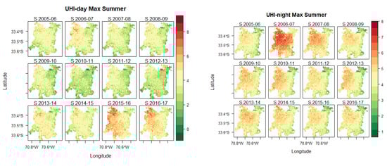
Figure 7.
Maximum daytime and nighttime UHIs for the 2005–2017 summer seasons. Each summer season considers the months of December from the previous year and January and February of the following year (e.g., S 2005–2006 means December 2005 and January and February 2006). The graph shows the maximum day and night temperatures over three months. During the maximum days in 2006–2007, there are high values mainly in the northwest, while at night during the same summer the UHI almost covers the entire city, probably due to the heat waves that occurred at that time. Conversely, during the summer days in 2015–2016 and 2016–2017, the UHI is higher than during the night.
During the summers of 2015–2016 and 2016–2017, daytime temperatures of the UHI increased to 8.5 °C, which could be a product of the large number of forest fires that occurred during summer 2015–2016 in the regions of Valparaiso and Metropolitan Santiago [55], as well as the mega forest fires that occurred during summer 2016–2017 [56]. During the night, except for summers 2006–2007 and 2007–2008, the heat island showed homogeneous behavior in extension and magnitude (Figure 7).
Regarding temperature variability of the UHI during the summers of 2005–2017 (Figure 8), the results demonstrate that there was minor variability in the southwest sector of the city, and large variations in the 2016–2017 summer in comparison with the rest of the summers. Nocturnal variation increases occurred in the northeast sector, mostly during the summers of 2006–2007 and 2007–2008. The variability magnitude was greater during the day than during the night, and a central nucleus was maintained during summer nocturnal periods.
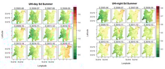
Figure 8.
Daily and nightly temperature dispersion of the UHI during each summer 2005–2017. Each summer season considers the months of December from the prior year and January and February of the following year (e.g., S 2005–2006 means December 2005 and January and February 2006). The graph shows the standard deviation of day and night temperatures over three summer months. There was greater dispersion in UHIs during the day than during the night (almost double), reaching the highest values in the summer of 2016–2017, followed by daytime UHIs in the summer of 2015–2016.
Finally, upon stratifying the UHI in three thermal ranges defined using the natural break method [57] (Figure 9), it can be observed that during the day and night of all studied summer periods, the temperature for the entire urban area was maintained above the rural temperature (i.e., within the heat island). The extension variation of the heat island during the day was in the range of 3–5 °C, slowly decreasing from summer 2005 to summer 2013 and eventually reaching nearly the whole urban area. Following the summer of 2013–2014, higher values occurred, increasing in magnitude and extension until 2017.
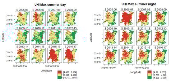
Figure 9.
UHI stratified in three ranges using the natural break method and daily and nightly data for summertime periods between 2005 and 2017. This graph shows a nocturnal UHI in 2006–2007 that decreases in extension during subsequent summers. On the other hand, during the daytime from 2013 to 2014, UHIs tend to increase, reaching the entire city in the summers of 2015–2016 and 2016–17.
The heat island presented its highest values during the night, but with less variability during the summer (a range of 3–5 °C). During the summer of 2006–2007, values surpassed the average maximum nocturnal temperature, although later they maintained a relatively stable behavior regarding extension and magnitude.
5. Discussion
The City of Santiago has a network of automatic meteorological stations of which eight are inside the city and one is outside of the city. The city currently has an approximate area of 837,892 km2 and a population density of 8497 people/km2. Therefore, the density of the automatic meteorological stations (AMS) network is 0.0096 AMS/km2, which is equivalent to one AMS per every 105 km2. This coverage is insufficient to carry out more detailed studies inside the city, especially for the spatial variability of air temperatures to be used in urban planning associated with the complexities of a city. In this sense, the scientific literature shows that the use of thermal satellite images improves the estimation of air temperature behavior inside the city, differentiating thermal configurations associated with the urban structure of the city [7,9,13,14].
The availability of free, medium-resolution, daytime and nighttime MODIS images aids research at a regional scale. Regarding the present study, we confirmed the existence of a relationship that allows air temperature modeling using satellite LST images with moderate resolution.
The observed values showed that the LST was always higher than the air temperature during each of the summers. However, they showed a regularity in each meteorological station on a daily level during each year as well. This regularity allowed us to find a simple linear relationship between LST and AT. However, this linear relationship was spatially explicit, which indicated that the regression coefficients were not constant in space but changed in accordance with other surface properties.
In the same way, altitude and NDVI variables improved the results in the spatially explicit regression models, achieving sufficient fit and significance levels.
The NDVI was used as an approximation regarding the surface state. For example, it allowed us to distinguish surfaces with or without vegetation. In addition, its relationship with surface emissivity allowed us to approximate its surface emission in a simple way.
To improve the temporal behavior modeling of the UHI and the thermal variations during the day and night, it is necessary to have data from validated weather stations that include equipment control systems and maintenance, as well as the availability of more stations distributed around the city.
The best adjustment and evaluation results for the day, night, and mixed linear models were obtained with day and night data used jointly (mixed), which is reflected in Table 3. In general, the determination coefficients found were relatively high, with a 0.72 mean value, a minimum value of 0.64, and a maximum value of 0.85, with an approximately variability of 8.7%. These values show that the applied method managed to capture an important percentage of the spatial behavior of the variable using a simple, but spatially explicit linear model via GWR, making it suitable for generating daily air temperature maps.
This UHI study in the city of Santiago provided some interesting results regarding the spatial variability of the air temperature modeled from the MODIS surface temperature (Figure 3b). For the spatial resolution of MODIS (1 km), it is possible to appreciate that the air temperatures were grouped into three well-defined spatial structures of homogeneous behavior (clusters) within the city and its surroundings. Additionally, this behavior was maintained approximately throughout the summer, but with some variations, as observed in Figure 4, Figure 5, Figure 6, Figure 7 and Figure 8. By classifying the UHI into three thermal ranges, it is possible to observe the thermal field variation and compare its extension during the study period (Figure 9). The first thing that can be observed is that, on average, the temperature inside the city was always higher than the surroundings (rural areas) during both the day and the night. If we compare urban and rural areas, the differences in air temperature were found to be in the range of 3 to 5 °C, showing variations between the years mainly due to interannual variability in the southern part of America.
The urban heat island in Santiago presents different daytime and nighttime behaviors. In the morning, the heat island has a marked presence in the northwest sector of the city. Although this area is less urbanized, because of the geological condition of its soils, it can quickly reflect, absorb, and emit incident solar energy [58]. The urban area, in contrast, can register morning temperatures less than those in natural environments, but this is reverted during the night due to thermal inversion. Morales [59] mentions that nocturnal radiative cooling of the surface generates an increment of 3 °C in the first 20 m above the ground, and that those that are coupled with thermal subsidence inversion are also present in the basin. On average, and throughout the study period, the nighttime UHI was more homogeneous than the daytime one, and had a greater spatial extension due to the low wind speed at night (Figure 4 and Figure 5). Also, the thermal difference between urban and rural areas was very noticeable since the city of Santiago has a highly urbanized landscape with few park areas when compared to the preferably agricultural environment. This difference between the city and its surroundings has an impact on the spatial variability of the UHI, which could affect AT estimates based on the linear model.
Considerable variations were not seen in the nighttime data (e.g., showing a cyclical condition or a marked rising trend in the magnitude of the UHI). For the daytime data, results showed variations in extensions as well as in magnitude: from December 2013 to the present, the heat island abruptly increased its extension, occupying the whole urban area. In both the summers of 2015–2016 and 2016–2017, a marked increase in magnitude was produced that could possibly be attributed to the large forest fires that covered the city with smoke for several days. These results agree with other studies on UHIs that present an increase in the extent of the UHI in several cities of China [60] or in the conterminous United States [61]. Although the changes in the extent of the UHI reported in this study cannot be explained or be directly associated with climate change (due to the short study period of 12 summer seasons), methodological development for later dates, as well as new satellite data, will complement this analysis, as climate change is expected to change the behavior of the UHI [62].
The study of UHIs through satellite imagery can be used as decision-making tools for urban planning and defining public policy. In this context, the presence of vegetative cover inside Santiago is suggested as an important control measure for the heat island [42]. However, marked differences in availability of funds mean that higher income sectors can invest more in private green areas. Meanwhile, sectors with fewer resources cannot access this control measure, and are therefore more directly affected by elevated urban temperatures [44].
High temperatures inside cities can negatively affect the economy. It is estimated that the total costs of climate change, considering UHIs, could be more than 2.6 times more for cities than in the previous century [63].
Finally, although the time period studied does not allow for conclusions about climatic variability, the extension and magnitude of the heat island registered at night during the last several summers (up to 9 °C), demonstrates a direct impact on the whole urban Santiago area, as well as on its inhabitants. This study improves the temporal resolution of previous studies in the study area [25] by being able to characterize and reveal the spatio-temporal patterns of the UHI, differentiating day and night effects.
6. Conclusions
The characterization of the UHI in Santiago de Chile was possibly due to the availability of free daily, medium resolution MODIS images (day and night), providing valuable information on trends within the city and its surroundings. However, the spatial resolution of the images was not enough.
In this study, the existence of a linear relationship between the AT and the MODIS surface temperature (LST) during the summer months was verified, observing a satisfactory agreement regarding the intensity and evolution of the thermal field during the summer period when the effect of UHI is strongest. Additionally, the verification of the altitude and NDVI variables adequately described the spatial variability of the linear regression coefficients, thereby improving the regression model results and achieving a spatially explicit orientation, which is expressed in satisfactory adjustments and significance levels [64]. It is possible that the unexplained variation in the relationship between LST and AT could be explained by the type of soil, its moisture content, and its use at a certain time. However, further investigation would be necessary to confirm this.
The UHI phenomenon must be adequately considered by urban planners in such a way that they can suggest mechanisms to municipalities for mitigating the effect of urban heat on populations. It is necessary to have thermal maps that express the spatial variability of UHIs in detail in order to plan the incorporation of new green areas in urban environments that might allow for better ventilation inside of cities during the summer.
The data and analysis retrieved from this study can be used to focus on public policies that address the UHI and the potential health issues it could cause in the population of the city of Santiago [31], such as thermal stress and its associated diseases (considering how some people in at risk groups are susceptible to the immediate heat effects, such as those people with advanced illness) [32].
Essentially, the results obtained show a possible urban planning application related to the prediction of approximate urban climates in summer months, as well as the thermal stress that the population may suffer within the city due to urban heat. This complementary information could be used to generate some of the climate change adaptation strategies that the Chilean government intends to put into practice in the next 50 years [65].
Future studies like this one, or with better spatial resolution data, will allow for a more adequate way of dealing with urban challenges, with an emphasis on improving urban planning, to mitigate surface temperature impact.
Author Contributions
Conceptualization, L.M.-S., J.S.R. and D.M.-F.; Methodology, L.M.-S., J.S.R. and D.M.-F.; Software, G.F.-J., D.M.-F.; Validation, D.M.-F., G.F.-J., and L.M.-S.; Formal Analysis, D.M.-F.; Investigation, L.M.-S., L.C.-J. and D.M.-F.; Resources, L.M.-S.; Data Curation, D.M.-F.; Writing-Original Draft Preparation, D.M.-F. and L.M.-S.; Writing-Review & Editing, D.M.-F., L.M.-S., J.S.R., L.C.-J., A.H., W.P.-M. and J.C.; Visualization, D.M.-F.; Supervision, L.M.-S. and W.P.-M.; Project Administration, L.M.-S. and L.C.-J.; Funding Acquisition, L.M.-S. and W.P.-M. All authors have read and agreed to the published version of the manuscript.
Funding
This research was supported by the National Fund for Scientific and Technological Development (FONDECYT), Chile (Project “Urban microclimate and human thermal comfort in urban spaces of the city of Santiago of Chile around university campuses”, Nº 1161809). The publication was made possible by the Publication Development Fund initiative of the Universidad Mayor.
Acknowledgments
This research was partially supported by the National Fund for Scientific and Technological Development (FONDECYT) and Publication Development Fund initiative, Universidad Mayor. Information and images on MODIS from 2005–2017 were obtained from https://lpdaac.usgs.gov/maintained by the NASA EOSDIS Land Processes Distributed Active Archive Center (LP DAAC), USGS/Earth Resources Observation and Science (EROS) Center, Sioux Falls, South Dakota, 2017. We are also grateful to Carolina Gallardo who reviewed this paper and, in that line, improved the manuscript significantly.
Conflicts of Interest
The authors declare no conflict of interest. The funders had no role in the study design; in the collection, analyses, or interpretation of data; in the writing of the manuscript, and in the decision to publish the results.
References
- Schär, C.; Vidale, P.L.; Lüthi, D.; Frei, C.; Häberli, C.; Liniger, M.A.; Appenzeller, C. The role of increasing temperature variability in European summer heatwaves. Nature 2004, 427, 332–336. [Google Scholar] [CrossRef] [PubMed]
- Melorose, J.; Perroy, R.; Careas, S. World population prospects. U. N. 2015, 1, 587–592. [Google Scholar] [CrossRef]
- United Nations, Department of Economic and Social Affairs, Population Division. World Urbanization Prospects: The 2014 Revision, Highlights (ST/ESA/SER.A/352); United Nations: New York, NY, USA, 2014; ISBN 9789211515176. [Google Scholar]
- Romero, H.; Sarricolea, P. Patrones y Factores de Crecimiento Espacial de la Ciudad de Santiago de Chile y Sus Efectos en la Generación de Islas de Calor Urbanas de Superficie. In Proceedings of the Clima, Sociedad y Medio Ambiente, V Congreso de la Asociación Española de Climatología, Zaragoza, España, 18–21 September 2006; Serie A N°. pp. 827–837. [Google Scholar]
- Álvarez, C.J.D. Metabolismo urbano: Herramienta para la sustentabilidad de las ciudades. Interdisciplina 2014, 2, 51–70. [Google Scholar] [CrossRef]
- Kennedy, C.; Cuddihy, J.; Engel-Yan, J. The Changing Metabolism of Cities. J. Ind. Ecol. 2007, 11, 43–59. [Google Scholar] [CrossRef]
- Arnfield, A.J. Two decades of urban climate research: A review of turbulence, exchanges of energy and water, and the urban heat island. Int. J. Clim. 2003, 23, 1–26. [Google Scholar] [CrossRef]
- Abutaleb, K.; Ngie, A.; Darwish, A.; Ahmed, M.; Arafat, S. Assessment of Urban Heat Island Using Remotely Sensed Imagery over Greater Cairo, Egypt. Adv. Remote Sens. 2015, 4, 35–47. [Google Scholar] [CrossRef]
- Taha, H. Urban climates and heat islands: Albedo, evapotranspiration, and anthropogenic heat. Energy Build 1997, 25, 99–103. [Google Scholar] [CrossRef]
- Lehoczky, A.; Sobrino, J.A.; Skoković, D.; Aguilar, E. The Urban Heat Island Effect in the City of Valencia: A Case Study for Hot Summer Days. Urban Sci. 2017, 1, 9. [Google Scholar] [CrossRef]
- Deilami, K.; Kamruzzaman, M.; Liu, Y. Urban heat island effect: A systematic review of spatio-temporal factors, data, methods, and mitigation measures. Int. J. Appl. Earth Obs. Geoinf. 2018, 67, 30–42. [Google Scholar] [CrossRef]
- Rivera, E.; Antonio-Némiga, X.; Origel-Gutiérrez, G.; Sarricolea, P.; Adame-Martínez, S. Spatiotemporal analysis of the atmospheric and surface urban heat islands of the Metropolitan Area of Toluca, Mexico. Environ. Earth Sci. 2017, 76, 137. [Google Scholar] [CrossRef]
- Sobrino, J.A.; Oltra-Carrió, R.; Sòria, G.; Jiménez-Muñoz, J.C.; Franch, B.; Hidalgo, V.; Mattar, C.; Julien, Y.; Cuenca, J.; Romaguera, M.; et al. Evaluation of the surface urban heat island effect in the city of Madrid by thermal remote sensing. Int. J. Remote Sens. 2012, 34, 3177–3192. [Google Scholar] [CrossRef]
- De Ridder, K.; Maiheu, B.; Lauwaet, D.; Daglis, I.A.; Keramitsoglou, I.; Kourtidis, K.; Manunta, P.; Paganini, M. Urban Heat Island Intensification during Hot Spells—The Case of Paris during the Summer of 2003. Urban Sci. 2016, 1, 3. [Google Scholar] [CrossRef]
- Nichol, J.E. A GIS-based approach to microclimate monitoring in Singapore’s high-rise housing estates. Photogramm. Eng. Remote Sens. 1994, 60, 1225–1232. [Google Scholar]
- Weller, J.; Thornes, E.J. An investigation of winter nocturnal air and road surface temperature variation in the West Midlands, UK under different synoptic conditions. Meteorol. Appl. 2001, 8, 461–474. [Google Scholar] [CrossRef]
- Keeratikasikorn, C.; Bonafoni, S. Urban Heat Island Analysis over the Land Use Zoning Plan of Bangkok by Means of Landsat 8 Imagery. Remote Sens. 2018, 10, 440. [Google Scholar] [CrossRef]
- Guiling, W.; Weimei, J.; Ming, W.E.I. An Assessment of Urban Heat Island Effect using Remote Sensing Data. Mar. Sci. Bull. 2008, 10, 14–25. [Google Scholar]
- Sobrino, J.A.; Irakulis, I. A Methodology for Comparing the Surface Urban Heat Island in Selected Urban Agglomerations Around the World from Sentinel-3 SLSTR Data. Remote Sens. 2020, 12, 2052. [Google Scholar] [CrossRef]
- Weng, Q. Thermal infrared remote sensing for urban climate and environmental studies: Methods, applications, and trends. ISPRS J. Photogramm. Remote Sens. 2009, 64, 335–344. [Google Scholar] [CrossRef]
- Mirzaei, M.; Verrelst, J.; Arbabi, M.; Shaklabadi, Z.; Lotfizadeh, M. Urban Heat Island Monitoring and Impacts on Citizen’s General Health Status in Isfahan Metropolis: A Remote Sensing and Field Survey Approach. Remote Sens. 2020, 12, 1350. [Google Scholar] [CrossRef]
- Kato, S.; Yamaguchi, Y. Analysis of urban heat-island effect using ASTER and ETM+ Data: Separation of anthropogenic heat discharge and natural heat radiation from sensible heat flux. Remote Sens. Environ. 2005, 99, 44–54. [Google Scholar] [CrossRef]
- Voogt, J. How Researchers Measure Urban Heat Islands. Dep. Geogr. Univ. West. Ontanrio 2007, 34. Available online: https://19january2017snapshot.epa.gov/sites/production/files/2014-07/documents/epa_how_to_measure_a_uhi.pdf (accessed on 22 September 2020).
- Zhang, P.; Imhoff, M.L.; Wolfe, R.E.; Bounoua, L. Characterizing urban heat islands of global settlements using MODIS and nighttime lights products. Can. J. Remote Sens. 2010, 36, 185–196. [Google Scholar] [CrossRef]
- Espinoza, P.S.; Martín-Vide, J.; Sarricolea, P. El estudio de la Isla de Calor Urbana de Superficie del Área Metropolitana de Santiago de Chile con imágenes Terra-MODIS y Análisis de Componentes Principales. Rev. Geogr. Norte Gd. 2014, 57, 123–141. [Google Scholar] [CrossRef]
- Tomlinson, C.J.; Chapman, L.; Thornes, J.E.; Baker, C. Derivation of Birmingham’s summer surface urban heat island from MODIS satellite images. Int. J. Clim. 2010, 32, 214–224. [Google Scholar] [CrossRef]
- Wan, Z. Collection-6 MODIS Land Surface Temperature Products Users’ Guide. 2013. Available online: https://lpdaac.usgs.gov/documents/118/MOD11_User_Guide_V6.pdf (accessed on 20 March 2017).
- Rizwan, A.M.; Dennis, L.Y.; Liu, C. A review on the generation, determination and mitigation of Urban Heat Island. J. Environ. Sci. 2008, 20, 120–128. [Google Scholar] [CrossRef]
- Dirección Meteorológica de Chile (DMC). Temperaturas en Santiago Marcaron un Nuevo Récord Histórico; DMC: Santiago, Chile, 2016. [Google Scholar]
- Subdere. Gobierno Regional Metropolitano División Administrativa de Chile. Available online: http://www.subdere.gov.cl/divisi%C3%B3n-administrativa-de-chile/gobierno-regional-metropolitano-de-santiago (accessed on 24 June 2017).
- Bell, M.; O’Neill, M.S.; Ranjit, N.; Borja-Aburto, V.H.; Cifuentes, A.L.; Gouveia, N. Vulnerability to heat-related mortality in Latin America: A case-crossover study in São Paulo, Brazil, Santiago, Chile and Mexico City, Mexico. Int. J. Epidemiol. 2008, 37, 796–804. [Google Scholar] [CrossRef] [PubMed]
- Muggeo, V.M.R.; Hajat, S. Modelling the non-linear multiple-lag effects of ambient temperature on mortality in Santiago and Palermo: A constrained segmented distributed lag approach. Occup. Environ. Med. 2008, 66, 584–591. [Google Scholar] [CrossRef]
- Peña, M.A. Relationships between remotely sensed surface parameters associated with the urban heat sink formation in Santiago, Chile. Int. J. Remote Sens. 2008, 29, 4385–4404. [Google Scholar] [CrossRef]
- INE—Instituto Nacional de Estadísticas. Censo de Población y Vivienda 2017. Available online: http://resultados.censo2017.cl/ (accessed on 22 June 2017).
- Busetto, L.; Ranghetti, L. MODIStsp: An R package for automatic preprocessing of MODIS Land Products time series. Comput. Geosci. 2016, 97, 40–48. [Google Scholar] [CrossRef]
- Estevez, J.; Gavilán, P. Procedimientos de validación de datos de estaciones meteorológicas automáticas. aplicación a la red de información agroclimática de andalucía. Inst. Investig. Form. Agrar. Aliment. 2008, 1–12. Available online: https://www.slideshare.net/LUISAQUIJEDIAZ/validacion-datos-estacion-meteo (accessed on 22 September 2020).
- Hooker, J.; Duveiller, G.; Cescatti, A. A global dataset of air temperature derived from satellite remote sensing and weather stations. Sci. Data 2018, 5, 180246. [Google Scholar] [CrossRef] [PubMed]
- Gutiérrez-Puebla, J.; Daniel-Cardozo, O.; García-Palomares, J.C. Regresión Geográficamente Ponderada (GWR) y estimación de la demanda de las estaciones del Metro de Madrid. In Proceedings of the XV Congreso Nacional de Tecnología de la Información Geográfica, AGE-CSIC, Madrid, España, 19–21 September 2012. [Google Scholar]
- Brunsdon, C.; Fotheringham, S.; Charlton, M. Geographically Weighted Regression. J. R. Stat. Soc. Ser. D 1998, 47, 431–443. [Google Scholar] [CrossRef]
- Soto Estrada, E. Regresión ponderada geográficamente para el estudio de la temperatura superficial en Medellín, Colombia. Rev. AIDIS 2013, 6, 42–53. [Google Scholar]
- Karnieli, A.; Agam, N.; Pinker, R.T.; Anderson, M.C.; Imhoff, M.L.; Gutman, G.G.; Panov, N.; Goldberg, A. Use of NDVI and Land Surface Temperature for Drought Assessment: Merits and Limitations. J. Clim. 2010, 23, 618–633. [Google Scholar] [CrossRef]
- Fábián, Z. Method of the Geographically Weighted Regression and an Example for its Application. Reg. Stat. 2014, 4, 61–75. [Google Scholar] [CrossRef]
- USGS. Global 30 Arc-Second Elevation (GTOPO30); USGS: Reston, VA, USA, 1996. [Google Scholar] [CrossRef]
- Emery, X. Apuntes de Geoestadística; Universidad de Chile: Santiago, Chile, 2013. [Google Scholar]
- LeGates, D.R.; McCabe, G.J. Evaluating the use of “goodness-of-fit” Measures in hydrologic and hydroclimatic model validation. Water Resour. Res. 1999, 35, 233–241. [Google Scholar] [CrossRef]
- Meek, D.W.; Howell, T.A.; Phene, C.J. Concordance Correlation for Model Performance Assessment: An Example with Reference Evapotranspiration Observations. Agron. J. 2009, 101, 1012–1018. [Google Scholar] [CrossRef]
- LeGates, D.R.; McCabe, G.J. A refined index of model performance: A rejoinder. Int. J. Clim. 2012, 33, 1053–1056. [Google Scholar] [CrossRef]
- Narita, D.; Tol, R.; Anthoff, D. Damage costs of climate change through intensification of tropical cyclone activities: An application of FUND. Clim. Res. 2009, 39, 87–97. [Google Scholar] [CrossRef]
- Willmott, C.J.; Ackleson, S.G.; Davis, R.E.; Feddema, J.J.; Klink, K.; LeGates, D.R.; O’Donnell, J.; Rowe, C.M. Statistics for the evaluation and comparison of models. J. Geophys. Res. Space Phys. 1985, 90, 8995. [Google Scholar] [CrossRef]
- DeLeeuw, J.; Akaike, H. Information Theory and Extension of the Maximum Likelihood Principle. In Proceedings of the 2nd International Symposium on Information Theory, Budapest, Hungary, 2–8 September 1973; Petrov, B.N., Csaki, F., Eds.; Akademia Kiado: Budapest, Hungary, 1973; pp. 267–281. [Google Scholar]
- Burnham, K.P.; Anderson, D.R. Model Selection and Inference—A Practical Information-Theoretic Approach; Springer Science & Business Media: New York, NY, USA, 1998; ISBN 9781475729191. [Google Scholar]
- Smith, P.; Aravena, H.R. Factores explicativos de la distribución espacial de la temperatura del aire de verano en Santiago de Chile. Rev. Geogr. Norte Gd. 2016, 63, 45–62. [Google Scholar] [CrossRef]
- Pebesma, E.; Benedikt, G. Spatial and Spatio-Temporal Geostatistical Modelling, Prediction and Simulation. Available online: https://mran.microsoft.com/snapshot/2017-02-04/web/packages/gstat/index.html (accessed on 12 April 2017).
- Reyes-Paecke, S.; Aldunce, I.M.F. Distribución, superficie y accesibilidad de las áreas verdes en Santiago de Chile. EURE 2010, 36, 89–110. [Google Scholar] [CrossRef]
- Actualización Onemi: Cinco Incendios Forestales se Mantienen Activos en Cinco Regiones del País. Available online: https://www.emol.com/noticias/Nacional/2016/01/31/786188/Actualizacion-Onemi-Cinco-incendios-forestales-se-mantienen-activos-en-cinco-regiones-del-pais.html (accessed on 30 September 2017).
- CONAF. Análisis de la Afectación y Severidad de los Incendios Forestales Ocurridos en Enero y Febrero de 2017 Sobre los Usos de Suelo y los Ecosistemas Naturales Presentes Entre las Regiones de Coquimbo y la Araucanía de Chile; Informe Técnico; Corporación Nacional Forestal: Santiago, Chile, 2017; p. 51. [Google Scholar]
- Jenks, G.F. The Data Model Concept in Statistical Mapping. Int. Yearb. Cartogr. 1967, 7, 186–190. [Google Scholar]
- Romero, H.; Molina, M. Relación espacial entre tipos de usos y coberturas de suelos e islas de calor en santiago de chile. An. Soc. Chil. Cienc. Geogr. 2008, 1, 223–230. [Google Scholar]
- Morales, R.G.E. Contaminación Atmosférica Urbana: Episodios Críticos de Contaminación Ambiental en la Ciudad de Santiago; Editorial Universitaria: Santiago, Chile, 2006; ISBN 9561118351. [Google Scholar]
- Qiao, Z.; Wu, C.; Zhao, D.; Xu, X.; Yang, J.; Li, F.; Sun, Z.; Liu, L. Determining the Boundary and Probability of Surface Urban Heat Island Footprint Based on a Logistic Model. Remote Sens. 2019, 11, 1368. [Google Scholar] [CrossRef]
- Li, X.; Zhou, Y.; Asrar, G.R.; Imhoff, M.; Li, X. The surface urban heat island response to urban expansion: A panel analysis for the conterminous United States. Sci. Total. Environ. 2017, 605, 426–435. [Google Scholar] [CrossRef]
- Alcoforado, M.J.; Andrade, H. Global Warming and Urban Heat Island. In Urban Ecology; Marzluff, J., Shulenberger, E., Endlicher, W., Alberti, M., Bradley, G., Ryan, C., Zumbrunnen, C., Simon, U., Eds.; Spinger: Boston, MA, USA, 2008; pp. 249–262. ISBN 9780387734118. [Google Scholar]
- Estrada, F.; Botzen, W.J.W.; Tol, R.S.J. A global economic assessment of city policies to reduce climate change impacts. Nat. Clim. Chang. 2017, 7, 403–406. [Google Scholar] [CrossRef]
- Gallo, K.; Hale, R.; Tarpley, D.; Yu, Y. Evaluation of the Relationship between Air and Land Surface Temperature under Clear- and Cloudy-Sky Conditions. J. Appl. Meteorol. Clim. 2011, 50, 767–775. [Google Scholar] [CrossRef]
- Ministerio Medio Ambiente de Chile. Estrategia Climática de Largo Plazo 2050. Available online: https://cambioclimatico.mma.gob.cl/estrategia-climatica-de-largo-plazo-2050/descripcion-del-instrumento/ (accessed on 10 September 2020).


© 2020 by the authors. Licensee MDPI, Basel, Switzerland. This article is an open access article distributed under the terms and conditions of the Creative Commons Attribution (CC BY) license (http://creativecommons.org/licenses/by/4.0/).