1. Introduction
Remote sensing has become an indispensable tool in forest management, due to the spatial scales of forested land and management timelines. The use of satellite or aerial imagery in land cover analysis enables land managers and planners to make landscape level decisions quickly and accurately. This is crucial for managers who work with large tracts of land, or researchers performing small-scale analyses. Advances in remote sensing introduce increasingly fine-resolution datasets, both spatially and spectrally. This allows more precise measures of variations across the landscape, such as forest species composition. Fortunately, many of these datasets are freely available for landscape analyses.
The relatively recent availability of sub-meter spatial resolution introduced new opportunities for precise measurements and predictions of land cover, allowing managers to identify land classes at a very fine scale. With the introduction of such high spatial and spectral resolution imagery, forest vegetation classification can be performed at species-level precision [
1,
2,
3]. Many recent studies conducted on species-level classification of forested landscapes make use of hyperspectral imagery with considerable success [
4,
5,
6,
7]. Fassnacht et al. (2016) found that hyperspectral sensors were used most frequently in tree species classification [
8]. Hyperspectral imagery provides an abundance of valuable information when distinguishing between vegetation classes but can be cost-prohibitive due to the lack of publicly available hyperspectral datasets. It can also come at the cost of spatial resolution, making fine-scale feature recognition difficult, such as the publicly available hyperspectral Hyperion dataset, which has a 30m spatial resolution. In temperate forests, multispectral datasets with NIR bands often provide sufficient spectral data to distinguish between vegetation classes [
3], especially when combined with light detection and ranging (LIDAR) data [
9]. The combination of lidar data with hyperspectral or multispectral data has been nearly universal in recent tree species classifications [
8]. Species-level classifications greatly benefit from the addition of lidar-derived height data [
4,
6,
10]. These data can be integrated at several different stages of the classification process [
11,
12].
Most recent studies have made use of non-parametric algorithms for tree species classification, particularly support vector machine and random forest (RF) [
5,
8,
9]. These algorithms do not assume normality within the dataset and allow a smoother integration of non-spectral data. While non-parametric algorithms generally produce the highest reported accuracies in tree species classifications, parametric algorithms like maximum likelihood (ML) are only surpassed in accuracy by a few percentage points in certain cases [
13,
14]. In some studies, a simple classifier is preferable, due to its low processing power requirements, user friendliness, and ease of access in many remote sensing software. Parametric classifiers are also suitable when ancillary data, such as spatial segmentation data, are not integrated into the algorithm [
15]. ML can even surpass non-parametric algorithms in highly heterogeneous regions when classifying aerial imagery alone [
14]. This is particularly true in very large study areas [
13].
As data quality progresses and improves, so do the classification techniques performed upon them. Many of the advances of the past few decades are concentrated in machine learning, the ultimate objective of which is to achieve or surpass the pattern recognition capacity of a human [
16]. Machine learning is a catch-all term that describes many different advanced algorithms used to perform difficult classifications or complex regressions [
17]. The complexity of machine learning algorithms covers a broad spectrum, from basic decision trees to “black box” deep neural networks. The success of advanced models is undeniable, as is evident in the abundance of recent publications showcasing the use of machine learning algorithms in land cover classifications [
5,
13,
18]. However, the complexity that makes these algorithms so effective also creates an obstacle to those with limited programming experience. High-level research certainly merits the use of such advanced techniques, but for a user with limited exposure to machine learning, can a more simplistic classification algorithm with extensive human training and oversight match the accuracy of an automated machine learning classification?
1.1. Unbalanced Data in Species Classification
When large swaths of land are captured by a sensor, the rich spectral information used for land-cover classification can be challenging for classes that covers only a fraction of the image. Therefore, we considered an unbalanced image one that contain classes with a number of pixels three orders of magnitude smaller than the rest of the classes [
19]. The presence of unbalanced data in species classification may be unavoidable for species that have a limited or unknown range within a large landscape. This is not an unusual occurrence for special status plant populations, as many species of high ecological value have rapidly declined in population size and spread. Additionally, as climate change affects species distribution, a larger study area might allow researchers to monitor the migration of the species into previously unpopulated areas, further contributing to an unbalanced distribution of the target class and background matrix. Several challenges arise when attempting to classify small, widely dispersed populations of a single species. There are two general methods of handling unbalanced classifications. The imbalance can be accommodated at the data level or the algorithm level, as reviewed by Ali et al. [
20]. This decision will affect the way that training and validation is sampled across classes, and may affect the algorithm selected. The creation of training and validation data is another difficulty, particularly if the species’ distribution is sporadic and difficult to predict. In this study, the target species is not necessarily limited to its natural preference of elevation and soil types, because the majority of Willamette Valley ponderosa pine is currently found in plantations, which may or may not occur within its historical range. These plantations can be found in forested, agricultural, or even developed environments, which make it difficult to fully eliminate regions in the search for training data. Class separability is another challenge in training a model with unbalanced class distribution, especially in species classifications. If the target species is not spectrally distinct from the background class(es) or otherwise clearly identifiable from auxiliary data such as height, it will be especially difficult to properly train the algorithm. Finally, the handling of accuracy measures must be tailored to the unbalanced classification. Most traditional algorithms are accuracy-centric, which can be artificially inflated by the correct classification of the non-target class. Metrics such as omission and commission error provide more insight into class-specific accuracy. For a holistic view of the classification accuracy, Cohen’s kappa coefficient, as discussed in
Section 2.7, is better suited than overall percent accuracy, as it represents the proportion of agreement between class accuracies, allowing the minority class greater representation in the metric.
1.2. Parametric and Non-Parametric Classification of Unbalanced Data
Many factors influence the suitability of parametric and non-parametric algorithms for vegetation classification. Species-level studies vary in study area, quantity and precision of classes, model complexity, time constraints, and desired product. The decision to use a parametric or non-parametric algorithm can be influenced by all of these factors. For species classifications that target one class of vegetation, unbalanced data, as discussed above, can introduce another challenge in selecting an appropriate algorithm.
Species classifications require algorithm training, and for large study areas that are broken into dozens or even hundreds of rasters, this can be time consuming. When building an unbalanced classification, analysts may attempt to create a representative sample of class training data in which the target species is known to occur in greater quantities, to classify a large assortment of rasters with unknown target species abundance. For datasets that are unequally distributed across the study area, creating a representative set of training data can be particularly time consuming. Non-parametric algorithms, such as decision trees or machine learning classifiers, are often selected for such tasks, as they are better equipped to handle unbalanced data through ensemble mechanisms such as bagging or boosting [
21]. The RF algorithm is among the most popular of these non-parametric classifiers, and generally is considered an improvement over traditional parametric supervised classification methods, such as ML. ML classifications also require a training dataset, but commonly the dataset is limited by its spatial relationship to the raster. Unlike RF, a generic training dataset is unsuitable for different spatial classifications when running an ML algorithm. Thus, a drawback of ML is the labor required to train the algorithm for each image. However, the level of detail required by ML can be one of its primary benefits when classifying an unbalanced dataset. The spectral signature of each class is represented more accurately for each raster, and the amount of variability within its spectral space is reduced. Significant variation can be found in a large aerial imagery dataset, due to atmospheric influences and flight timing. Parametric classifications may reduce the impacts of these variations by using training data exclusive to each individual raster being classified, while non-parametric classifications may require some accepted reduction in training data accuracy, or additional pre-processing, such as atmospheric or light correction.
1.3. Ponderosa Pine in the Willamette Valley
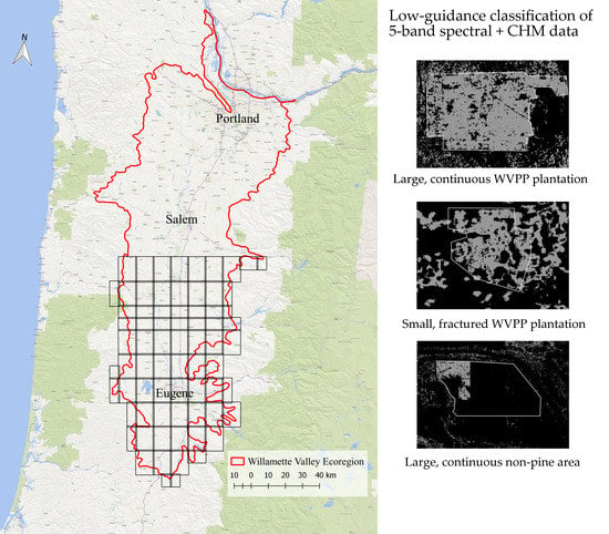
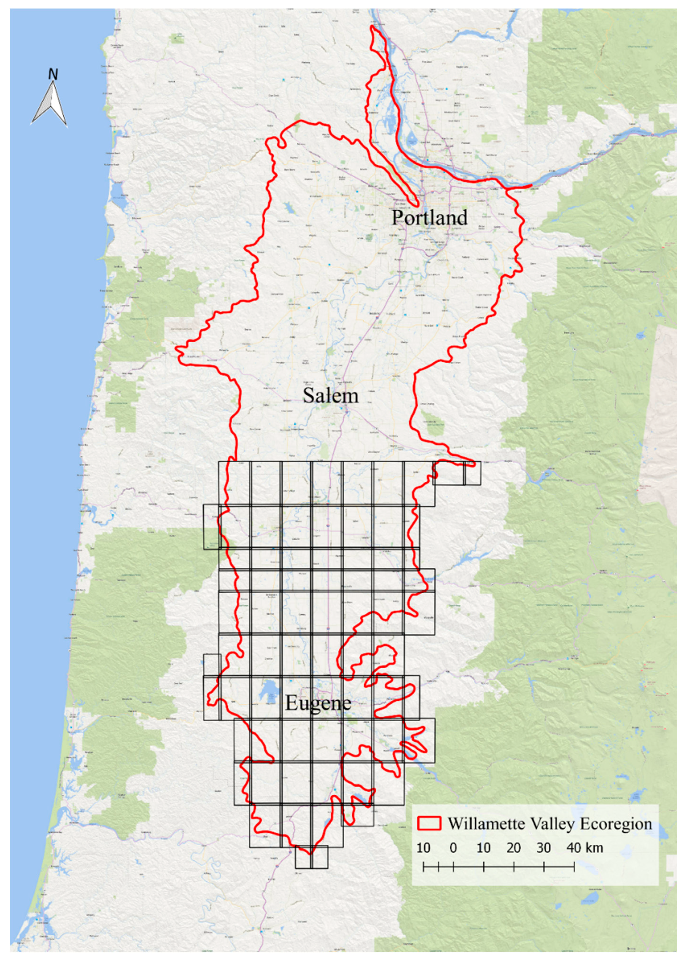
The Willamette Valley is located in northwestern Oregon (
Figure 1), a region composed of agriculture, developed urban areas, and temperate forest. Douglas-fir (
Pseudotsuga menziesii) dominates the majority of surrounding forests of the Willamette Valley, often growing with western hemlock (
Tsuga heterophylla), western redcedar (
Thuja plicata), and deciduous trees such as bigleaf maple (
Acer macrophylla) and red alder (
Alnus rubra). While these species are among the most common today, this was not the case prior to European settlement of the region.
Historically, indigenous communities burned large areas of the valley to maintain an abundance of edible plant species and to maintain visibility for hunting. The routine burning minimized the growth of trees and hardwood shrubs, creating an abundance of open prairies. Surveyors noted that Willamette Valley Ponderosa Pine (WVPP) typically grew within white oak (
Quercus garryana) woodlands, shallow hills and ridges, areas prone to flooding, and in open savannahs with white oak and Douglas-fir [
22,
23]. These forest types were most likely maintained by the routine burning by indigenous tribes [
24]. However, the settlement of the Willamette Valley in the 1880s resulted in an almost complete conversion of prairie and open woodlands to agriculture and Douglas-fir forest by inhibiting natural and human-induced forest fires. Most WVPP stands were harvested for building materials as development expanded, resulting in just a few scattered stands of native pine. These stands are often found on three soil types: Poorly drained clay in flat areas or foothills; shallow, rocky clay in foothills; and in well-drained sandy areas in the Willamette River floodplain [
25]. Natural regeneration of WVPP has been limited primarily by low light conditions in historically suitable locations [
23].
In 1996, a group of concerned landowners and researchers formed the Willamette Valley Ponderosa Pine Conservation Association (WVPPCA) with the intention of maintaining the genetic diversity of WVPP and increasing the ease of acquiring and growing the pine locally [
25]. The WVPPCA has located over 900 native WVPP stands, with 150 individual trees serving as seed stock sources to preserve and propagate. However, the extent of younger WVPP plantations, most having been planted after the advent of the WVPPCA, is still unknown. Methods explored by this study may be used to quantify the current extent of WVPP. To identify the most suitable methods for area prediction, we compare the accuracy and the trade-offs between parametric and nonparametric classifications in the context of a small-scale land assessment with open-source data.
2. Materials and Methods
2.1. Study Area
The Willamette Valley is an alluvial region in northwestern Oregon of about 14,457 km
2 [
26]. It is bounded by the Coast Range to the west and the Cascade Range to the east, encompassing the Columbia River to the north and ending around the Klamath Mountains to the south. The true ecoregion includes a small portion of southwestern Washington, but for the purpose of this research, the northern boundary was clipped to the Oregon-Washington border. The shapefile delineating this region was acquired through the Oregon Spatial Data Library [
27]. The southern half of the Willamette Valley level III ecoregion of Oregon, which encompasses the study area [
28,
29], is approximately 8166 km
2.
The center of the valley is primarily developed urban and agricultural land, and encompasses several large cities, including Portland, Salem, and Eugene. Nutrient-rich soil and relatively flat topography (sea level to 122 m) makes the Willamette Valley a significant agricultural area. The Valley contains several prominent rivers, including the Columbia, Willamette, Tualatin, McKenzie, Santiam, and others. The perimeter of the valley rises into the foothills of the Coast and Cascade Ranges, where dense forests take over the landscape. Most WVPP has been planted at the interface of rural urban areas and commercial forestland.
2.2. Data
2.2.1. Aerial Imagery
High-resolution red-green-blue-infrared (RGBI) aerial imagery was acquired from the National Agriculture Imagery Program (NAIP), which is flown every two to three years in all continental states. The data were collected using Leica Geosystem’s ADSH100/SH100 digital sensors, flown on a Cessna 441 at a height of about 8400 m. The sensors recorded imagery at 40cm or 80cm GSD in four wavelengths, namely red, green, blue, and near-infrared. Images were captured continuously at three angles: Nadir, forward (26°), and backward (19°). Flight lines were oriented north/south with 30% sidelap.
The data were processed to contain four RBGI bands with a ground pixel resolution of 1 m. The imagery was delivered as georeferenced digital ortho-quarter quad tiles (DOQQ), each tile covering one USGS topographic quadrangle. The Willamette Valley ecoregion contained 507 orthophotos collected in June and August of 2016 with no cloud cover. Two hundred and thirty-one of these raster images fell within the focus area of the southern Willamette Valley. However, only a small fraction contains Ponderosa pine that could be reliable identified from the images. Therefore, we have focused the study on five DOQQ tiles, which covered an area of 69,722 hectares.
The training data was partially created through known locations of WVPP, but most sites were identified by visually scanning aerial imagery for WVPP-specific characteristics, such as color, crown structure, and planting patterns. This process was facilitated by a false color composite of the NAIP imagery and very-high-resolution satellite reference imagery. Across the used dataset, 12.8 ha of WVPP training regions were identified and used. An additional two or three classes were used in parametric classification to hone the pine training areas, namely non-pine coniferous forest and low vegetation classes were used for all classifications, and a deciduous class was used in riparian-dominated regions. For non-parametric classifications, only two classes were used (pine and non-pine). The training data for the additional classes were created using visual assessment of the NAIP imagery, as they were less spectrally precise than the WVPP regions.
2.2.2. Lidar
Lidar-derived highest hit digital surface models (DSMs) and bare earth digital elevation models (DEMs) of the focus area were acquired from the State of Oregon Department of Geology and Mineral Industries. The majority of data used was collected in the 2009, with some additional data from the 2012, 2015, and 2016 [
30].
Watershed Sciences, Inc. collected and processed the lidar data for the 2009 projects. The data were flown using a Leica ALS50 Phase II laser system mounted in a Cessna Caravan 208. Data were collected at near nadir, and flight lines overlap 60% to 75% laterally. The average pulse density in 2009 was 8.14 pulses per m2 with an average ground density of 1.36 returns per m2. The project average relative accuracy was 0.050m, and root mean square error for the calculated absolute accuracy was 0.04 m. The DSMs were created using highest hit lidar data, and the DEMs were created using triangular irregular networks (TIN) processing of ground point returns using TerraScan and Microstation.
2.2.3. Species Cover Maps
Estimated species cover datasets have been created for western Oregon and surrounding regions in the Pacific Northwest, such as the gradient nearest neighbor (GNN) species map created by the Landscape Ecology, Modeling, Mapping, and Analysis (LEMMA) group. LEMMA’s species map provides a continuous raster image of estimated plant community composition over large landscapes [
31]. Likelihood of species composition is calculated by pixel proximity to the nearest of approximately 25,000 plots, and the climate, soil, geographic, and topographical conditions of the pixel. The raster image has a spatial resolution of 30m. The accuracy of the model is highly variable, with a reported kappa of 0.00–0.80 for species presence or absence. Each pixel represents an “ecological system” containing multiple associated species, usually a mix of tree and understory vegetation.
The inherently mixed species pixels of this dataset limit its usefulness in training or validating a single-species classification map, especially a species such as WVPP, which is present in small quantities within a very fragmented matrix of agricultural, forested, and developed land covers, and often occurs in very small stands that may be lost in the 30 m resolution of the GNN map. However, in future studies of unbalanced species mapping, a GNN species map may be very useful in providing a preliminary filter that can mask out unsuitable vegetation communities in large study areas.
2.3. Aerial Imagery Pre-Processing
Initial attempts to run an ML classification on the original NAIP aerial imagery resulted in a high level of noise and class blending. The high spatial resolution of the imagery led to wide spectral variation within each target class, causing substantial overlap between the vegetation classes. To decrease spectral variability within the classes, a smoothing filter was applied to each image before classification. This filter came from the Orfeo Toolbox “Mean-Shift Smoothing” algorithm, which draws spatial and spectral information from neighboring cells within given radii to produce an image that preserves integral edges [
26]. Although this algorithm is typically used for image segmentation, full segmentation was not performed for this project because of the scale and complexity of the dataset. The addition of object data information would contain errors and would not have provided meaningful separability to the pine and non-pine forest classes.
2.4. Enhancing Spectral Data
2.4.1. Canopy Height Model (CHM) Band Incorporation
The original NAIP imagery data had limited class separability potential. Although the spatial resolution was very high—so high that the smoothing filter was needed—the spectral resolution was limited to four bands. Many tree species classification studies make use of multispectral or hyperspectral data with much higher spectral resolution [
5,
6,
7,
18]. Studies that have similar spectral limitations usually enhance the imagery with spatial or structural data [
9]. As noted by Fassnacht et al. (2016), the majority of recent tree species classification publications have incorporated lidar data into the classification at the pixel level [
8]. For this study, we created canopy height models (CHMs) by subtracting the DEMs from the DSMs, which provided a normalized representation of the true feature heights in the dataset. Fassnacht et al. (2016) claim that CHMs can be of limited use when fused with spectral data pre-classification, a finding supported by Ghosh et al. (2014), who did not notice any significant improvement in classification accuracy when fusing lidar-derived height data with hyperspectral data [
7]. However, we chose to test this claim in the context of height data fusion with low spectral resolution data. The CHM was added to the NAIP imagery as a fifth band, incorporating the lidar data at the decision level, as described by Shen [
11].
2.4.2. CHM Mask Application
In an additional test of the effectiveness of CHM data in vegetation class separation, we created CHM-based height masks to apply post-classification. Our goal was to reduce commission of agricultural and mature conifer regions. The CHM rasters were reclassified, with values between 5 feet and 90 feet assigned a value of one, and all other heights assigned a value of zero. The minimum value was selected to exclude areas of low, non-forest vegetation while preserving young WVPP stands, and the maximum value was selected to exclude mature, non-pine conifer stands. This range exceeds the expected height of most planted WVPP stands, because most stands targeted by this study are under 30 years old as a result of the conservation efforts of the 1990s [
32]. However, the 90-foot ceiling was established because mature conifers tend to be more spectrally similar to WVPP than young conifers, and conifers often reach heights within this range upon maturity. We assumed that conifers under 90 feet would be spectrally distinct from WVPP. These masks were applied to the 4-band and 5-band classifications of both parametric and non-parametric methods. Lidar data were not available for the entire extent of the classified focus area. For no-data lidar regions, the 4-band classification data were used. In areas with available lidar data, we multiplied the 4- or 5-band parametric or non-parametric classified rasters by the CHM mask rasters. This raster algebra assigned a value of zero to areas that fell outside the acceptable height range, while areas that fell within the positive mask range maintained their original classification value.
2.4.3. Vegetation Index Band Incorporation
In a preliminary attempt to increase class separability, we tested the impact of incorporating two vegetation indices as fifth bands: The normalized difference vegetation index (
NDVI) and the visible-band difference vegetation index (
VDVI), similar to Wang Xiaoqin et al. [
27].
The
NDVI and
VDVI are calculated with pixel values and do not rely on sensor-specific coefficients, such as the enhanced vegetation index. The
NDVI and
VDVI are extensively used in unmanned aircraft systems (UAS), which do not experience significant atmospheric interference, and often only collect visible band imagery, due to the wide availability of high spatial resolution cameras [
33]. We predicted that
NDVI would help differentiate drought-tolerant WVPP from moisture-adapted conifers in the Valley, and that
VDVI would help accentuate the visible color variations between WVPP plantations and other tree species. This trial was carried out on a smaller subset of rasters than the CHM band addition and mask application.
2.5. Parametric Classification
2.5.1. Algorithm Selection for Parametric Method
To identify the WVPP using the parametric method, we chose three algorithms based on their popularity in image analysis: ML [
34], minimum distance (MD) [
35], and spectral angle mapper (SAM) [
36]. The three algorithms were initially assessed based on their ability to delineate the WVPP from the spectral RGBI data only. We selected, for further analysis, the most accurate algorithm, the accuracy being measured in this situation by the correctly identified pines and the size of the false positives. Each trial used identical training datasets to classify the same raster, and the required parameters were tuned through trial and error. The large size of the aerial imagery dataset recommended a classification method that uses a spectral library to classify the dataset, rather than developing training data specific to each image. SAM has this capability, so an additional training dataset of pine, non-pine mixed conifer, and non-forest vegetation was compiled with samples across the southern Willamette Valley. We performed a second trial of SAM classification on the sample region using this spectral library training dataset.
2.5.2. ML Classification Process
The ML algorithm distributes pixels among the classes based on the probability of class membership. The version of ML used in the study uses non-normalized discriminant function
gi(
x) rather than true probabilities [
37]:
i = class
x = n-dimensional data (where n is the number of bands)
p(ωi) = probability that class ωi occurs in the image and is assumed the same for all classes
|Σi| = determinant of the covariance matrix of the data in class
Σi−1 = its inverse matrix
mi = mean vector
To allocate a pixel to a class, the discriminant functions are compared with the threshold, which leads to the inequality:
where
Ti is the threshold for class
ωi.
The rearrangements of terms from (4) ends with a separation that can be interpreted in probabilistically:
In eventuality that
x is normally distributed,
follows a χ
2 distribution with the degrees of freedom equal the number of bands [
37]. The χ
2 distribution helps in deciding whether a pixel belong to a class or not, as larger values of
place the pixel in the tail of the distribution. In our study, we have selected the thresholds by choosing the probability of rejecting a pixel from a class thru trial and error. We found that a value of 5% for the probability of rejecting a pixel as belonging to a class supplies the expected results, irrespective of the class. Therefore, the thresholds were computed as:
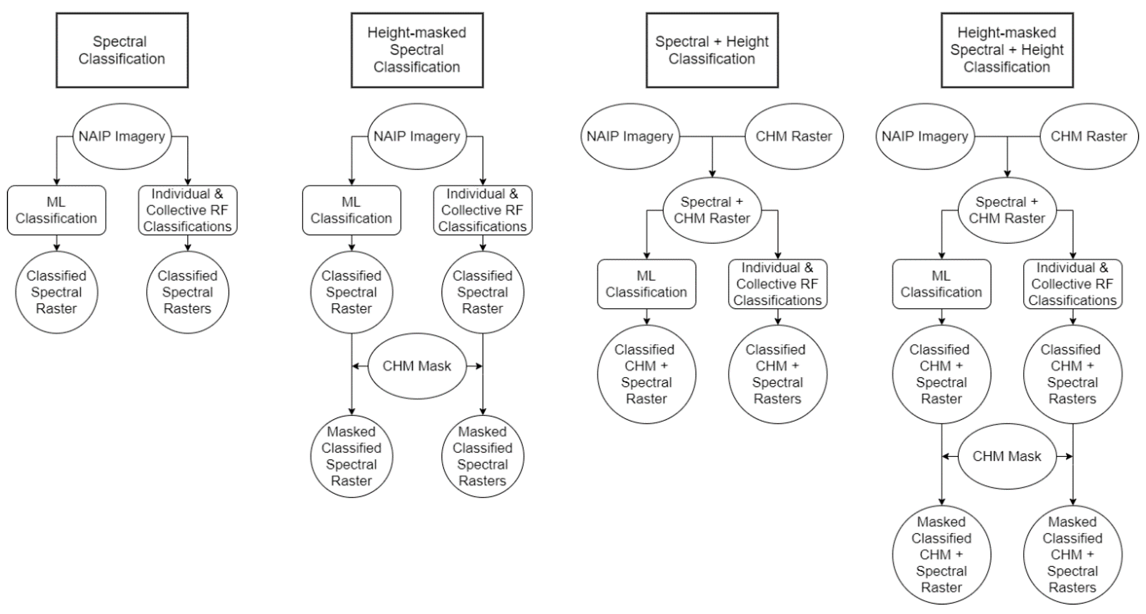
The ML classifications were performed using the ENVI implementation of the ML algorithm, which was applied on the enhanced NAIP imagery with and without the CHM mask on the four-band spectral NAIP data and the five-band NAIP + CHM data. Therefore, a set of four ML classifications were executed (
Figure 2).
2.6. Non-Parametric Classification
The ML classifier is not the only algorithm that provides accurate results for image analysis [
14,
38]. Decision trees, or ensemble methods, are another tool often used for image classification [
39,
40,
41]. Among decision tree methods, RF is likely the most popular [
42,
43,
44]. RF is a non-parametric stochastic supervised learning algorithm suitable for image classification [
45,
46,
47]. Mirroring most supervised classification algorithms, RF contains a training phase during which multiple decision trees are built. The results produced by each decision tree are aggregated, and the output is the class with the largest number of occurrences. The RF algorithm has the ability to correct for overfitting [
46,
48], a property not common to other machine learning algorithms, such as neural networks [
49,
50]. Toloşi and Lengauer [
51] pointed out that even though the RF algorithm is robust to multi-collinearity and overfitting, its accuracy likely depends on the relationship between the number of features and the number of samples. Among the available implementations of the RF algorithm, we selected the randomForest package, which is an R enactment of the original code written by Breiman and Cutler in Fortran [
52]. The RF algorithm depends on a multitude of parameters [
53], chief among them being the number of trees and the number of variables used at each split of a tree. To identify the most appropriate values, we have run a factorial experiment with four levels for the number of trees (i.e., 100, 200, 300, and 400) and three levels for the number of variables used at each split of a tree (i.e., 2, 3, and 4).
Mirroring the ML method, we performed four RF variations within the non-parametric classification method. The 4-band NAIP and 5-band NAIP + CHM rasters were classified in R, and the CHM binary mask was applied to each of these (
Figure 2).
Irrespective of the classification approach (i.e., parametric or non-parametric), the NAIP images were proven to provide superior results than classifications applied on images with lower spatial resolution [
54], such as Landsat. The reduction of the pixel size can increase the classification accuracy by more than 10% compared with larger pixels, as it will be able to delineate classes such as shade or ground [
55,
56,
57]. Smaller pixels are able to capture landscape details invisible to larger pixels; therefore, they are more adequate to delineate spectral signatures within the ponderosa pine plantations, particularly the ground. Considering that the crown of the trees will cover most of the ground, the sparse non-pine pixels within the plantation are easily separated by using contiguity and minimum surface constraints.
2.7. Training, Validation, and Accuracy Assessment
The NAIP images used for assessment contain less than 0.02% of identified ponderosa pine. Because of the relatively low abundance of WVPP in naturally or artificially mixed stands, and the difficulty in validating the accuracy of a classified mixed stand, only plantations that would provide an uninterrupted signature of WVPP were considered for training and validation. Across the 69,722 ha of the area, all of the 12.8 ha of pine pixels were used to train and validate the classifiers, with a randomized 7:3 ratio of training to validation pine stands. For the ML parametric classifier, we randomly selected non-pine pixels covering 86.3 ha. Because of the reduced, unbalanced presence of the pine in the study area, there were no assessment data outside the 12.8 ha, meaning that the accuracy was carried out on the validation data. For each tile and classification method, a set of three randomizations were executed, which produced 243 combinations, i.e., 35.
We assess the performances of the nonparametric classifier RF with a 5-fold cross-validation approach, similar to Goetz et al. [
58] and Heung et al. [
59]. Each run was executed by splitting the pixels identified as ponderosa pine 70% for training and 30% for validation, as recommended by Chicco [
60]. Considering the unbalanced data, we have considered four sample sizes for the non-pine class, all reported to the size of pine class: the same, twice as large, 10 times larger, and 100 times larger. Because the images were acquired in slightly different illumination conditions, we conducted the non-parametric classifications via two strategies: One in which the RF classification was carried out on each image, independently (i.e., training and validation from one image at a time), and one in which the RF classification was executed by combining all the images (i.e., training and validation data extracted from all images simultaneously).
All classifications were assessed using overall accuracy, kappa coefficient, and pine commission and omission error (Equations (4)–(7)) [
61,
62]. We placed a significant emphasis on the overall accuracy, because of the unbalanced ratio of non-pine area to pine area (at least 100 times according to Mueller-Warrant et al. [
56] and 1000 times according to the selected study area). For the unbalanced data, the kappa coefficient is a more suitable metric for accuracy assessment, because it accounts for the uneven distribution of the pixel among classes. Although pine commission and omission error provide a one-sided perspective on the classification abilities, they do supply a precise metric for our objective.
where:
TP = number of pixels with pine predicted with pine (true positive)
TN = number of pixels without pine predicted without pine (true negative)
FP = number of pixels without pine predicted with pine (false positive)
FN = number of pixels with pine predicted without pine (false negative)
All = total number of pixels: All = TP + TN + FP + FN
4. Discussion
4.1. Spectral Data Enhancement
The addition of height data to the NAIP aerial imagery at both pixel level (included in classification) and decision level (included post-classification) improved classification accuracies across all variations of parametric and non-parametric methods. The incorporation of vegetation indices had minimal effects upon the accuracy of the preliminary ML classification, and in fact reduced overall accuracy and kappa for two of the three index combinations. The number of indices that were available for use were extremely limited, as EVF and other indices requiring band coefficients have not yet been established for NAIP imagery. NDVI and VDVI use simple band algebra to emphasize differences in vegetation reflectance. Such indices can be valuable in reducing excess spectral information and exaggerating differences between classes, but when classified in combination with all original input bands, there is little to no new information added to the pixel stack. The minor improvement in overall accuracy offered by the NDVI band did not provide sufficient evidence for its usefulness in class separation, and the decrease in accuracy among the other index combinations supported our decision not to include these indices further.
4.2. Parametric Classification and the Effects of CHM Incorporation
The four-band ML classification on average had the lowest accuracy of all classification methods (67.73% overall accuracy and 0.29 kappa coefficient). This low average can be attributed to several influences. The biggest challenge for the four-band classification is the difficulty to represent the pine class fully, with its spectral variations introduced by age and tree heath, while also excluding all other types of vegetation. Additionally, each raster contains varying quantities of pine, exacerbating the difficulty in adequately representing the pine class within each raster when few stands are available to be sampled. Images with fewer pine stands available, consequently training data, generally produced worse results.
The accuracy of the four-band classification was greatly improved by applying the CHM mask, primarily by its removal of pine commission in the non-forest vegetation class. By masking the four-band ML classified images, mean pine commission was reduced by about 29%, resulting in an overall accuracy of 83.14% and kappa coefficient of 0.51. Visually, the similarities between WVPP stands and certain agricultural crops are stronger than the similarities between WVPP stands and other deciduous or coniferous forest species, making the lower height mask of five feet particularly effective.
Incorporation of the CHM band to create the five-band had a similar, but slightly weaker effect on the ML classification in terms of average overall accuracy and kappa coefficient. However, pine class commission was reduced by a substantial 41%, while pine class omission was reduced by about 3%. Masking cannot truly affect pine omission, as the mask does not add any pixels excluded from the pine class. Any decrease in pine omission from masking is the result of masking a different iteration of the four-band or five-band classified image. This large decrease in pine commission suggests that the ML algorithm was successfully able to remove non-pine areas that matched the spectral signature but did not match the average height of the pine training areas. Some of these non-pine areas that were ultimately included may have been included at the fringe of the class parameters, lacking a hard limit in height parameters. There may have been points within the pine training data that fell outside the 5 to 90-foot limit, creating leeway in height discrimination.
While the generalized accuracy metrics suggest that a mask application is more effective in isolating the pine class, the substantial decrease in pine commission in the five-band classification compared to the mask’s effect on commission reinforces the impact of the unbalanced data. Because the non-pine class is an amalgam of every single land cover other than pine, its less impressive accuracy lowered the overall accuracy and kappa of the five-band classification, while the mask automatically transferred any pixels outside of height range to the non-pine class, boosting its accuracy automatically.
The steady improvement in accuracy throughout the ML methods suggests that neither incorporation of CHM data should be ruled out in a parametric classification. Certainly, a combination of spectral and height bands is superior to an entirely spectral classification, but the application of a decision-level height mask helps correct excess commission error within a binary classification, even when the same data are incorporated at the pixel level. This is particularly visible in the jump from 0.47 to 0.89 kappa coefficient between the unmasked and masked five-band ML classification.
4.3. Non-Parametric Classification and the Effects of CHM Incorporation
The four-band RF classification applied to individual images surpassed the accuracy of the four-band ML classification by nearly 30%, achieving an average overall accuracy of 95.63% (
Table 6). This incredible increase in accuracy speaks to the effectiveness of non-parametric algorithms in classifying pure spectral data. While the four-band RF classification was quite impressive, increases in accuracy were practically inexistent with the addition of height data, as opposed to the dramatic increases seen between ML methods.
The application of the height mask to the four-band classification was effectively null, while the incorporation of the CHM band as the five-band raster improved accuracy by a scant 0.33% (0.01 kappa). Pine omission and commission were likewise weakly improved. A slightly larger, but otherwise negligible improvement was made by masking the five-band classification.
We found that better accuracy was achieved when classifying images with their own spatially related training data (individual classification) as opposed to a collective classification (
Table 7). This is likely due to the spectral variability between images, which has a pronounced effect upon the attempt to separate the precise spectral signatures of varying vegetation species. The minimum accuracy for collective classification was more than 5% smaller than the smallest accuracy obtained for individual images (
Table 7), even that the standard deviation was almost the same (i.e., 0.021). The decrease in accuracy with more than 2% from individual images to all the images is probably the results of the RF accounting for the increase variability associated with the larger landscape considered simultaneously rather than separately. The reduction in the ability of the RF to delineate ponderosa pine over large areas, which inheritably have not only larger variability but also was recorded from different position of the sun and atmospheric conditions, was present in the omission and commission errors, which also increased with more than 2% compared with the classification of individual images (
Table 6 and
Table 7). The addition of CHM did not improve the accuracy (i.e., 93.43% vs. 93.36%) but reduced the variability (i.e., standard deviation decreased from 0.0205 to 0.0203, meaning 1%), even insignificantly.
4.4. Parametric v. Nonparametric Accuracy
While the RF algorithm generally outperformed the ML method in most variations in terms of overall accuracy, most notably when classifying four-band spectral data, the accuracies of ML and RF began to converge with the application of CHM data through pixel-level fusion and mask application in the ML classifications. Overall accuracies were nearly equal between the five-band masked classifications by each algorithm, with a slightly lower kappa for ML (
Table 5). The use of CHM data in the ML classifications was particularly effective in reducing commission in the pine class. This came at the price of increasing pine omission, which is visible in
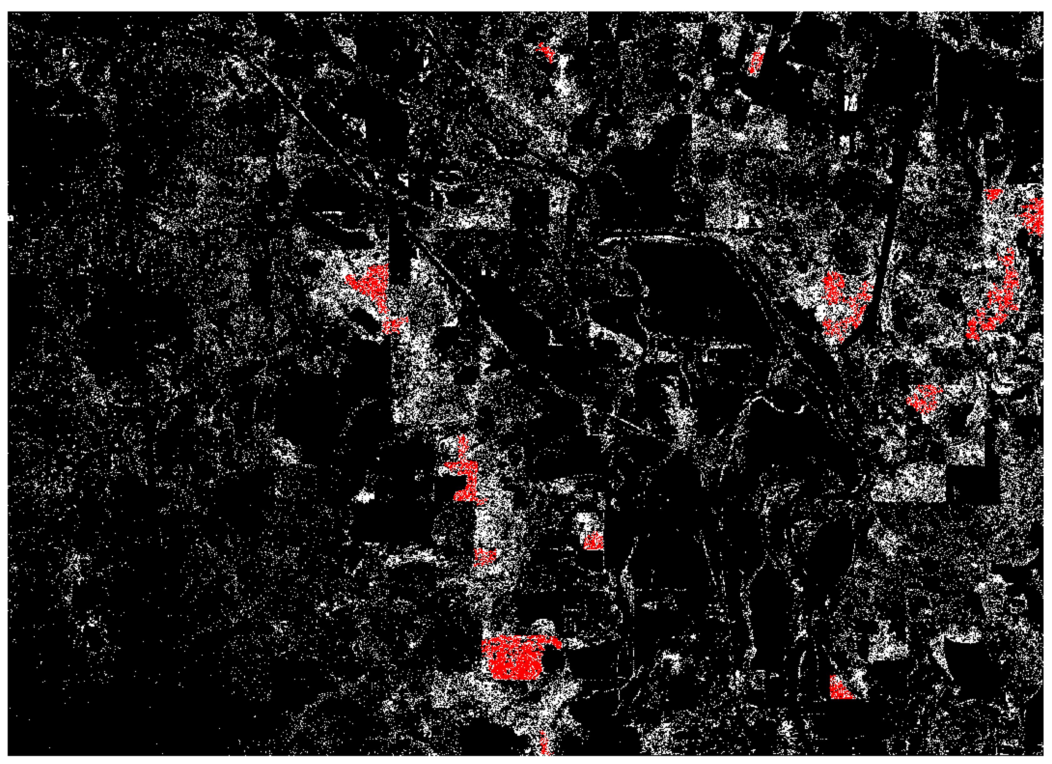
Figure 3 and
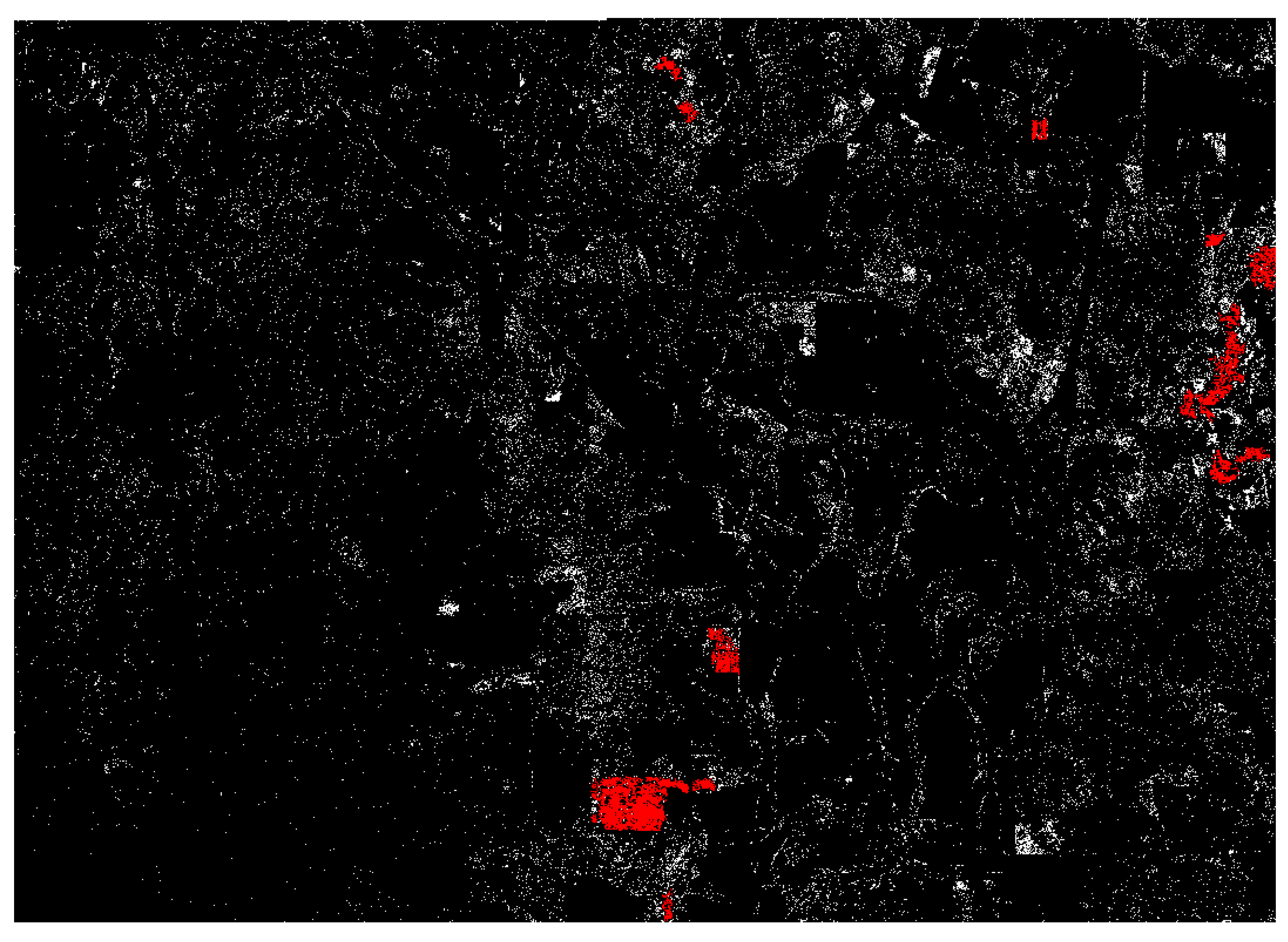
Figure 4; the ML image is much less dense than the RF image. The contiguous pine stands were not classified as completely by ML as they were by RF, and therefore were highlighted by a larger sieve for the ML image (areas greater than 1000 m highlighted for ML, areas greater than one hectare highlighted for RF).
When classifying large areas, the acquisition of training and validation regions can be tedious. While the collective RF classifications were technically lower in accuracy than the individual classifications, the differences were small enough that a collective RF classification could require a lower density of training data across the landscape, enabling the user to accurately classify regions where training data are scant or non-existent. This is a major drawback of ML, which requires that training data be provided from the image to be classified.
The unbalanced proportion of WVPP in respect to the rest of the land use classes was successfully identified by the selected parametric and non-parametric algorithm. However, the non-parametric algorithm provided results that were consistently superior to the parametric algorithm, even if the difference in overall accuracy was operationally negligible. The non-parametric algorithm had a kappa coefficient consistently larger than 0.90—values unattained by the parametric algorithm. Nevertheless, the only situation when the two types of algorithms were comparable were when the elevation data were included, which in many areas is not available. In the case when only spectral data are available, the non-parametric algorithm is superior in binary classify landscapes with highly unbalanced vegetation classes.
4.5. Sources of Error
The limited spectral resolution, large size of the imagery dataset, and the unbalanced targeted classes contributed to many of classification errors. Considering that the training data could not be fully ground-verified, it is likely that some of the pine training regions that could not be verified with street-view imagery were not truly pine but were instead Douglas-fir or another spectrally or structurally similar species. Furthermore, the training data could only be obtained by visual assessment of the imagery, rather than in-person sampling. In as many cases as possible, we only used training data that could be validated through street-view imagery. However, these data are not available in rural parts of the study area, so for some regions, training data were created solely through assessment of high-resolution satellite imagery in various color composites. Some training data were composed of plantations that may have been too thin to provide a solid spectral signature, thereby including understory pixels that contributing to pine commission. Age differences between pine stands also contributed to spectral variability within the pine class.
The most common confusion was between pine and mixed-conifer plantations that shared similar planting and growth patterns, and certain agricultural crops. Widely spaced Douglas-fir plantations, especially mature Douglas-fir, is visually similar to many WVPP plantations. As WVPP and Douglas-fir stands age, they become more similar spectrally. WVPP stands tend to have a duller, browner reflectance than other conifer stands. This is partially because WVPP is planted at a wider spacing and has low-density crown characteristics, resulting in a higher proportion of ground visibility within the stand and through the canopy. We aimed to minimize this confusion through the integration of CHM data with the spectral data.
5. Conclusions
We found that the highest accuracies, considering overall average, kappa coefficient, omission, and commission, are achieved by fusing CHM data with spectral data and performing a non-parametric classification, followed by a height mask. However, if height data are not available for the area of interest, a non-parametric classification of spectral data alone provides near-equivalent results.
If a parametric algorithm is to be used, the classification is dramatically improved through the addition of height data and masking, as the addition of non-spectral data offers greater class separability in spectrally similar areas. Because our classification targets were forest stands rather than individual trees, height data of moderate resolution was useful and more readily available for such a large study size. The unbalanced nature of the dataset was sufficiently handled through under-sampling of the majority non-pine class.
RF was the superior classification method for our data, because the non-parametric algorithm was ultimately the best fit for the unbalanced, non-parametric nature of our study area. Isolating such a small segment of the spectral landscape within a massive study area required the on-the-fly adaptations of RF, while ML was limited by our defined classes and training areas.
Although RF classification of five-band imagery achieved the highest accuracies of the six methods, the ML method still reached a reasonably high kappa coefficient and extremely low commission rates with the addition of the CHM mask. While RF is the preferable method when classifying small-scale, high-resolution aerial imagery, the ML method can still achieve high accuracies if height data is available to enhance it.
Our findings suggest that the parametric and non-parametric method used in the study are appropriate for unbalanced binary classifications. However, the non-parametric algorithm is better suited for heterogeneous land cover, and if necessary, can be modified to use a standardized training dataset on an iteration of images, whereas the parametric method requires training data that are spatially related to each image in the iteration. The non-parametric method seems to be suitable for both standalone spectral and height-fused data, although the addition of height data may increase the classification accuracy across nearly all metrics.


