Short-Range Elastic Backscatter Micro-Lidar for Quantitative Aerosol Profiling with High Range and Temporal Resolution

Abstract

A bi-static short-range elastic backscatter micro-lidar, named Colibri, has been developed for quantitative aerosol profiling with high range and temporal resolution within the first hundred meters. The geometric (i.e., overlap) and radiometric (i.e., lidar constant) calibrations were performed along with dark current and background noise characterizations. Results of a measurement campaign have demonstrated the capability of our system to characterize aerosol plumes with high range-resolution (<10 cm) in the short-range close to their emission sources (from 10 m). To this aim, fog-oil aerosol plumes were generated in a tunnel and characterized by using an optical particle counter. A forward inverse method without boundary conditions is presented for inverting short-range lidar profiles when no reference molecular zone is available. Lastly, we report the different retrieved lidar products, namely the distribution of aerosol layers, radiative properties (i.e., backscatter profiles), and the microphysical properties (i.e., number concentration profiles). For the validation of the proposed methodology, the lidar products were compared with measurements from the optical particle counter. Lastly, the impact of calibration errors on the lidar products is discussed through an uncertainty analysis.

1. Introduction

Aerosols are suspended particulate matter in the atmosphere and are emitted through a wide range of natural or anthropogenic processes and play an important role in the Earth’s radiative balance. Elastic backscatter lidars are good candidates for range-resolved monitoring of aerosols as they provide quantitative properties of aerosols. This is important information for a wide range of applications including environments, air quality, climate change assessment, and space studies [1,2,3,4,5]. While traditional atmospheric aerosol lidars were designed for long-range measurements, they generally remain blind in the short-range, within typically the first thousand meters, due to incomplete overlap between the laser beam and the receiver field of view.

A recent need has been raised for short-range elastic backscatter lidars with high range-resolution and temporal-resolution to characterize aerosols close to their emission sources by decreasing the minimal measurement height [6,7,8]. These profiles are valuable in the fields of environment and air quality for accurate modeling of aerosol dispersion during events such as industrial plumes [9,10] or aerosol events in the atmospheric boundary layer (ABL) [11,12,13,14]. Short-range micro-lidars are showing new possibilities for aerosol research in aero-spatial and defense where accurate measurements of aerosol properties with high spatial-resolution are required to assess the performances of the optronic systems in adverse environmental conditions [15,16,17,18]. For instance, these systems are especially useful in characterizing obscurants such as fog, or smoke plumes, which may cause undesirable effects for active optronic systems [19,20,21]. Yet, up to now, aerosol lidars remain scarce for probing the atmosphere in the first hundred meters with a range-resolution lower than one meter.

ONERA, The French Aerospace Lab, has developed a short-range elastic backscatter micro-lidar dedicated to high range-resolution aerosol profiling. The system has been specifically designed to provide quantitative aerosol profiles with centimeter range resolution within the first hundred meters. The aims of this work are: (i) to demonstrate the capability of our system to characterize aerosol plumes with high range-resolution in the short-range close to their emission sources, (ii) to present a forward inverse method without boundary conditions dedicated to short-range lidar profiles when no reference molecular zone is available, and (iii) to present the different retrieved lidar products: the distribution of aerosol layers, radiative properties (i.e., backscatter profiles), and the microphysical properties (i.e., number concentration profiles). This paper is organized as follows. The system description and calibration, as well as the proposed inverse method, are reported in Section 2. Experimental results from field experiments are presented in Section 3 and are discussed in Section 4 to assess the performances of the Colibri micro-lidar. Finally, the concluding remarks and perspectives are presented in Section 5.

2. Material and Methods

The general lidar framework, along with notations and useful lidar-relevant quantities, is briefly outlined in this section.

2.1. Framework

The returned lidar signal for bi-static and multi-axial systems originates from the two-way attenuated backscattering by particles in the atmosphere at an angle determined by the transmitter–receiver geometry [22]. The elastic lidar equation under the single-scattering approximation assumes that the incident wave is scattered only once and multiple-scattering events are excluded. This well-known equation can be directly derived from the radiative transfer equation and can also be seen as the link-budget that provides the backscattered power $\mathrm{P}\left(\mathrm{r}\right)$ at a given range r as:

$$\mathrm{P}\left(\mathrm{r}\right)={\mathrm{K}}_{\mathrm{o}}\mathrm{O}\left(\mathrm{r}\right)\mathrm{U}\left(\mathrm{r}\right){\mathrm{r}}^{-2}\left[\mathrm{W}\right]$$

(1)

where:

K${}_{\mathrm{o}}$ is the radiometric lidar constant which depends on the transmitted laser pulsed energy ${\mathrm{E}}_{\mathrm{o}}$ or power ${\mathrm{P}}_{\mathrm{o}}$, the duration of the laser pulse $\tau$, and the receiver aperture area A as:

$$\begin{array}{cc}\hfill {\mathrm{K}}_{\mathrm{o}}& ={\mathrm{P}}_{\mathrm{o}}\frac{c\tau }{2}\mathrm{A}={\mathrm{E}}_{\mathrm{o}}\frac{c}{2}\mathrm{A}[W·m^3·sr]\hfill \end{array}$$

(2)

O(r) is the range-dependent overlap function which is a correcting function for measurements where the field of view of the receiver does not completely overlap the emission beam.

U(r) is the attenuated backscattering function defined as:

$$\mathrm{U}(\mathrm{r})=\beta \left(\mathrm{r}\right)\exp \left(-2{\int }_0^{\mathrm{r}}\alpha \left({\mathrm{r}}^{\prime }\right)\mathrm{d}{\mathrm{r}}^{\prime }\right)[{\mathrm{m}}^{-1}{\mathrm{sr}}^{-1}]$$

(3)

with $\alpha \left(\mathrm{r}\right)$ and $\beta \left(\mathrm{r}\right)$ are the total extinction and backscattering coefficients defined as:

$$\beta (\mathrm{r})=\sum _{\gamma =\mathrm{aer},\mathrm{mol},\mathrm{sur}}{\beta }_{\gamma }(\mathrm{r})[{\mathrm{m}}^{-1}{\mathrm{sr}}^{-1}]\alpha (\mathrm{r})=\sum _{\gamma =\mathrm{aer},\mathrm{mol}}{\alpha }_{\gamma }(\mathrm{r})[{\mathrm{m}}^{-1}]$$

(4)

where the subscripts aer,mol, and sur describe the aerosol, molecular, and surface components, respectively. For sake of clarity, the wavelength dependence of these parameters is omitted.

Different physical quantities must be derived from light-scattering for retrieving the lidar products of interest. The aerosol extinction and backscattering coefficient profiles, ${\alpha }_{\mathrm{aer}}$ and ${\beta }_{\mathrm{aer}}$, are derived from the aerosol extinction and differential backscattering cross-sections $C^{\mathrm{ext}}$ and $\mathrm{d}{C}^{\mathrm{bac}}$ as:

$${\alpha }_{\mathrm{aer}}\left(\mathrm{r}\right)={\int }_{{\mathrm{R}}_{\min }}^{{\mathrm{R}}_{\max }}{\mathrm{N}}_{\mathrm{p}}(\mathrm{r},\mathrm{R})C^{\mathrm{ext}}(\mathrm{r},\mathrm{R})\mathrm{d}\mathrm{R}[\mathrm{m}{}^{-1}]$$

(5)

$${\beta }_{\mathrm{aer}}\left(\mathrm{r}\right)={\int }_{{\mathrm{R}}_{\min }}^{{\mathrm{R}}_{\max }}{\mathrm{N}}_{\mathrm{p}}(\mathrm{r},\mathrm{R})\mathrm{d}{C}^{\mathrm{bac}}(\mathrm{r},\mathrm{R})\mathrm{d}\mathrm{R}[\mathrm{m}{}^{-1}\mathrm{sr}{}^{-1}]$$

(6)

where ${\mathrm{N}}_{\mathrm{p}}$ is the aerosol or particle number concentration per unit volume of an isotropic scattering medium formed by an ensemble of randomly oriented particles of radius R with ${\mathrm{R}}_{\min }$ and ${\mathrm{R}}_{\max }$ the minimum and maximal radii. Consequently, these aerosol cross-sections are the key radiative quantities for aerosol lidar applications [23] and are essential for evaluating microphysical properties such as aerosol number concentration from lidar profiles. The particle extinction cross-section $C^{\mathrm{ext}}$, expressed in unit of surface area, and differential backscattering cross-section $\mathrm{d}{C}^{\mathrm{bac}}$, expressed in unit of surface area per unit of solid angle, are defined as:

$$C^{\mathrm{ext}}(\mathrm{r},\mathrm{R})=Q^{\mathrm{ext}}(\mathrm{r},\mathrm{R})C^{\mathrm{geo}}(\mathrm{r},\mathrm{R})\left[m^2\right]$$

(7)

$$\mathrm{d}{C}^{\mathrm{bac}}(\mathrm{r},\mathrm{R})={\left(\frac{d{\sigma }^{\mathrm{sca}}(\mathrm{r},\mathrm{R})}{d\mathsf{\Omega }}\right)}_{\theta =\pi }=\frac{1}{4\pi }{Q}^{\mathrm{bac}}(\mathrm{r},\mathrm{R})C^{\mathrm{geo}}(\mathrm{r},\mathrm{R})[\mathrm{m}{}^{-1}\mathrm{sr}{}^{-1}]$$

(8)

where $Q^{\mathrm{ext}}$ is the extinction efficiency, $Q^{\mathrm{bac}}$ is the backscattering efficiency and $C^{\mathrm{geo}}$ is the geometrical cross-sections defined as $\pi {\mathrm{R}}^2$ for a spherical particle of radius R. The particle extinction can be seen as the modification of the energy flow along the forward direction due to scattering and absorption [24]. Note that the differential scattering cross-section $d{\sigma }^{\mathrm{sca}}/d\mathsf{\Omega }$ is expressed in unit of surface area per unit of solid angle.

The under-determination of the lidar problem, i.e., the retrieval of two unknowns parameters from only one lidar measurement, appears in Equation (3). The inversion of this ill-posed problem requires an intrinsic relationship between the backscattering and extinction cross-sections. A common practice is to assume that these two cross-sections are simply related in the form of ratio named Lidar Ratio (LR) or extinction-to-backscattering ratio [25,26,27]. This intensive lidar parameter, i.e., which does not depend on the concentration of particles, is defined for aerosols as:

$$LR(\mathrm{r},\mathrm{R})=\frac{C^{\mathrm{ext}}(\mathrm{r},\mathrm{R})}{\mathrm{d}{C}^{\mathrm{bac}}(\mathrm{r},\mathrm{R})}=4\pi \frac{Q^{\mathrm{ext}}(\mathrm{r},\mathrm{R})}{Q^{\mathrm{bac}}(\mathrm{r},\mathrm{R})}\left[\mathrm{sr}\right]$$

(9)

This lidar ratio strongly depends on the size, shape, or composition of particles. This fact can be established from lidar campaigns [28,29,30] or light-scattering models accounting for irregularly shaped-particles [31,32,33,34]. In this work, the latter was adopted. For the molecular contribution, we report the reader to [35,36] for further references.

The surface backscattering coefficient, ${\beta }_{sur}$, can be calculated under the assumption of an extended Lambertian target that intercepts the entire laser beam. From Kavaya et al. from [37], the analytical expression of ${\beta }_{sur}$ is expressed in unit of surface area per unit of solid angle as:

$${\beta }_{sur}(\mathrm{r})=\frac{2}{c\tau }{f}_r\left({\theta }_i\right)\delta \left(\mathrm{r}\right)[\mathrm{m}{}^{-1}\mathrm{sr}{}^{-1}]$$

(10)

where $\delta \left(\mathrm{r}\right)$ is the delta-function and $f_r\left({\theta }_i\right)$ is the Bidirectional Reflectance Distribution Function (BRDF) of the reference surface defined for an incident angle ${\theta }_i$ as:

$$f_r({\theta }_i)=\frac{\rho }{\pi }cos\left({\theta }_i\right)[\mathrm{sr}{}^{-1}]$$

(11)

where $\rho$ is the Directional-Hemispherical Reflectance (DHR) of the surface.

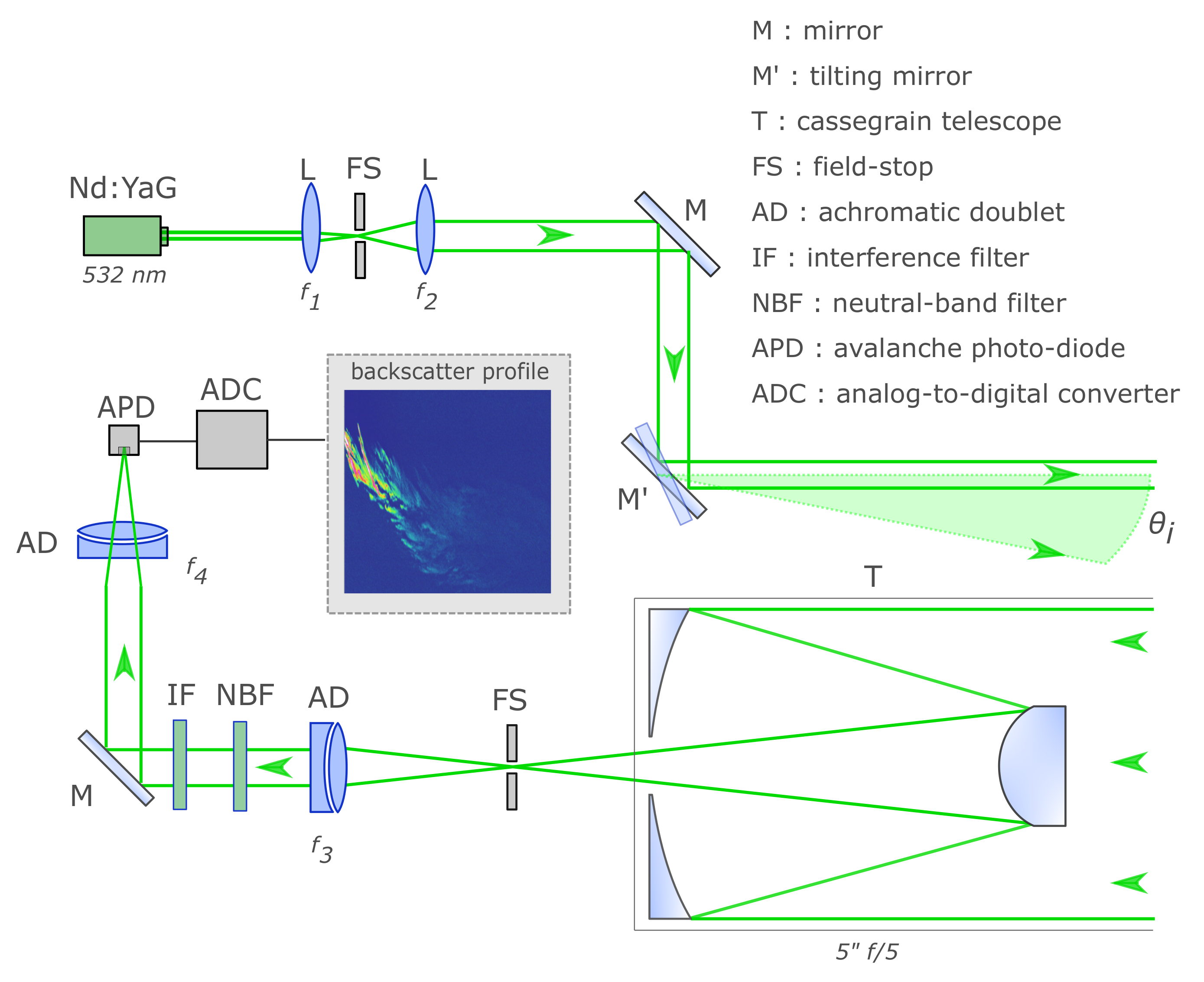
2.2. System

The Colibri micro-lidar is a forward-pointing elastic-backscatter lidar designed to characterize aerosols plumes (e.g., cloud, fog, soot). The function of this instrument is to perform remote measurements of particulate media in the short-range within the first hundred meters with high range-resolution of 10 cm along the line of sight and high-temporal resolution up to 1 measurement per millisecond. The micro-lidar architecture is bi-static and multi-axial with scanning capability in order to ensure measurements in the short-range. The system is lightweight, compact, and suitable for a mobile platform. The instrument optical layout is depicted in Figure 1 and its specifications are summarized in

Table 1. Specifications of the Colibri micro-lidar.

Laser	Wavelength	532 nm
	Pulse duration	<800 ps
	Pulse repetition rate	1.0 kHz
	Pulse energy	20 $\mathsf{\mu }$J
	Beam divergence	0.5 mrad
	Beam diameter	1 mm
	Bi-static angle	1–5 mrad
Receiver	Type	Cassegrain
	Effective diameter	90 mm
	Focal length	500 mm
	F-number	6.3
Sensor	Type	Si-APD
	Bandwidth	1.0 GHz
	Responsivity	15 A/W
	Active area	0.2 mm${}^2$
Digital Signal Processing	Bandwidth	>1.5 GHz
	Resolution	12 bits
	System control	Embedded computer

. The system is based on different units described in the following.

The transmitter unit is composed of a compact air-cooled Nd:YAG laser that emits 800 ps light-pulses of 20 $\mathsf{\mu }$J at the wavelength of 532 nm with a repetition rate of 1 kHz and a divergence of 0.5 mrad. The linear-polarized laser beam is reflected and directed towards the aerosols of interest using a scanning aluminum mirror (M’). A bi-static architecture was preferred over mono-static configuration to prevent laser pulses to cause internal reflections that could overwhelm the optical sensor and thus reduce the minimum range of measurement. The bi-static angle, i.e., the angle ${\theta }_i$ subtended between the transmitter and receiver units, is an essential feature for short-range measurements as it enables full control of the overlap function.

The receiver unit employs a Cassegrain telescope with an effective diameter of 90 mm and focal length 500 mm to collect the backscattered light from particulate media. The light collected by the telescope is then focused on the sensing unit using an ensemble of achromatic doublet (AD), neutral-band filter (NBF), interference filter (IF), mirrors (M). For short-range measurements, the ensemble after the telescope is placed on a translation stage, allowing the adjustable position of the lidar focal plane. Short-range lidar measurements rely on this essential feature to compensate for defocus problems when probing scattering volumes at small distances. In all the measurements reported here, the focal plane position is set to maximize the collected signal at approximately 30 m.

The sensing unit receives the focused backscattered light on the photosensitive surface of a high-bandwidth silicon avalanche photodiode (Si-APD). A high bandwidth single-channel Digital Signal Processing (DSP) unit digitizes the pre-amplified analog signal from the Si-APD. The digitized signal is transferred to a computer for processing and retrieving of lidar products.

The retrieval of radiative and microphysical properties of aerosol plumes from elastic backscatter micro-lidar in the short-range requires a different methodology than usual atmospheric elastic lidar systems. Proper calibration of the micro-lidar is essential and can be decomposed into two distinct calibration processes:

(i)

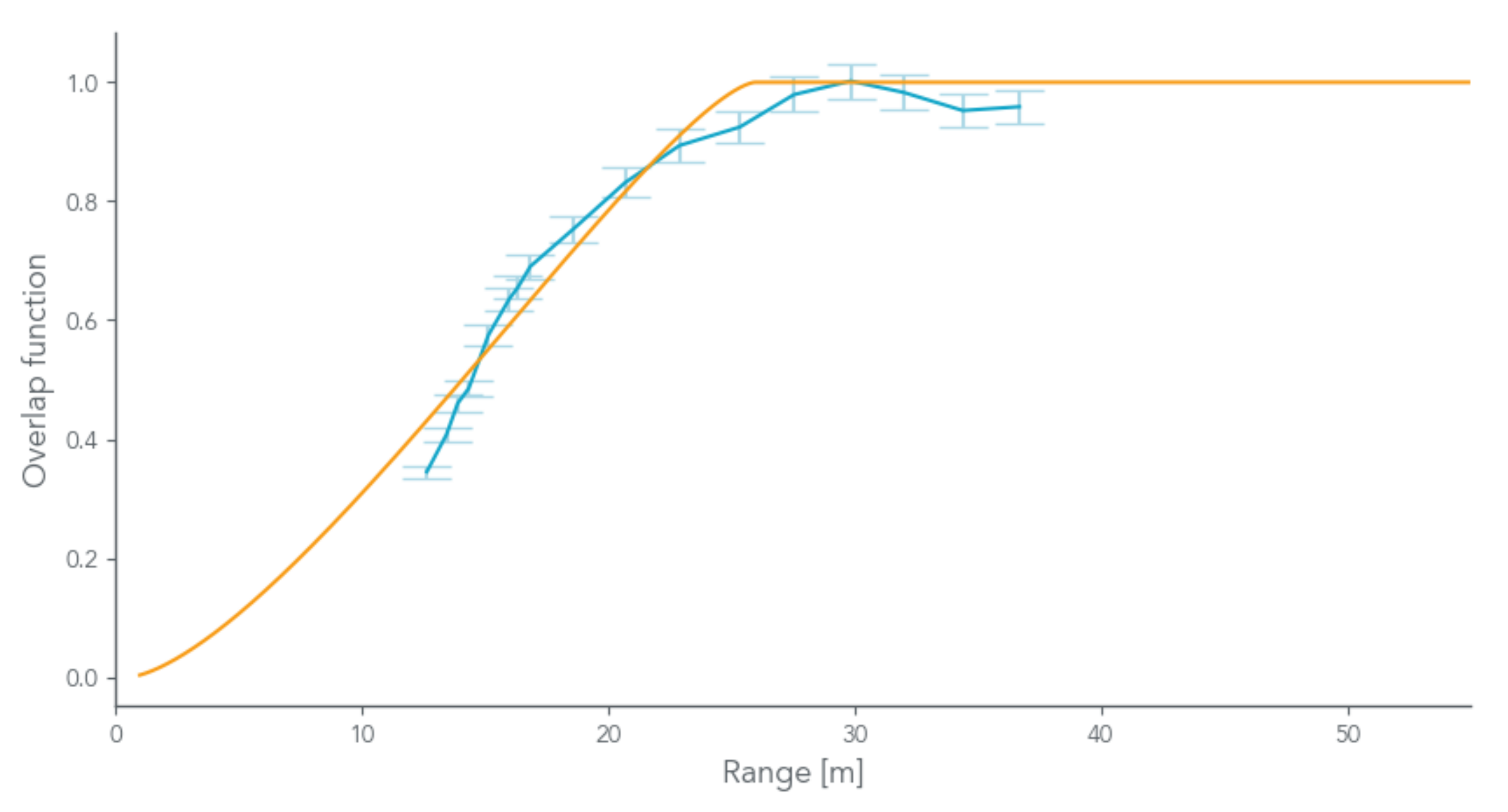
Geometric calibration, which is necessary for determining the overlap function of the lidar, especially in the short-range;

(ii)

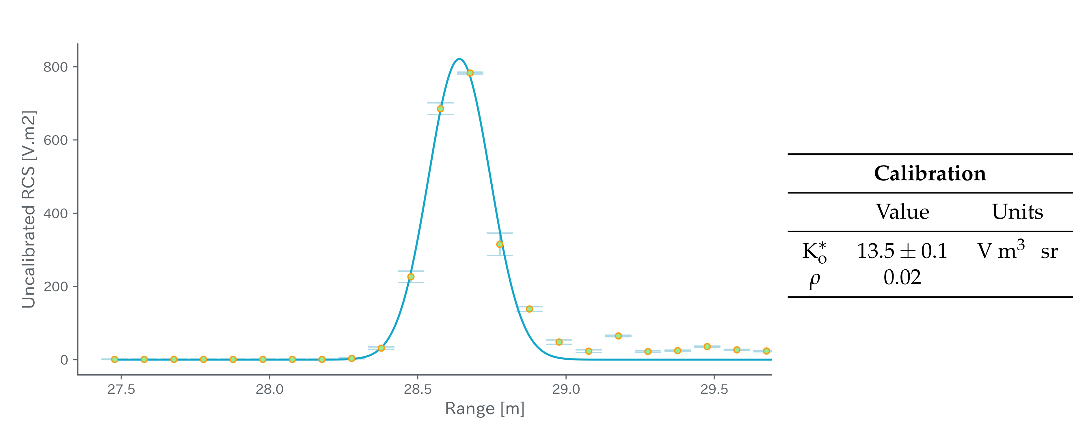
Radiometric calibration, which is required for retrieving the attenuated backscatter profiles and to use dedicated inverse methods that do not require any knowledge of boundary conditions or reference zone (e.g., Fernald–Klett methods).

2.3. Calibration

A critical problem for performing short-range measurements with elastic backscatter lidar arises from the incomplete overlap between the lidar transmitter and receiver. This incomplete overlap problem is a major source of uncertainty for profiling aerosol radiative and microphysical properties with short-range lidars. From an instrumental perspective, it can be seen as a lidar collection efficiency that varies with range. The origin of this variation originates from the changes of the image-plane position with the range of the scattering volume, which affects the efficiency of the lidar collection. As a result, the light backscattered by aerosols in the short-range may not completely reach the optical sensor. This zone is often referred to as the lidar incomplete overlap or blind zone. Nevertheless, a wide range of techniques has been proposed to determine the overlap function of lidar systems. Theoretical methods [38,39] require complete knowledge of all the lidar specifications with sufficient accuracy. Because such accurate information is generally not available for most lidar systems, experimental approaches have been undertaken to estimate the overlap function [40,41,42,43,44,45,46].

The Colibri micro-lidar was specially designed with a bi-static multi-axial configuration for profiling aerosols in the short-range with a reduction of the incomplete overlap zone. An evaluation of the range-dependent overlap function is proposed using a simple two-step method. First, a series of lidar measurements on a low reflectance Lambertian surface (Spectralon, Labsphere) are carried out at different ranges. Second, an analytical function reported by Stelmaszczyk et al. [47] is used to fit the measurements using the bi-static lidar parameters. The advantage of our method based on low reflectance surfaces is that it does not rely on the usual assumption of homogeneous atmospheres used for estimating the overlap function. To prevent any damages of the photodetector due to intense reflection on the surface, a neutral density filter may be inserted without affecting the geometric calibration.

Figure 2 reports the experimental evaluation of the overlap function for a series of ranges in the short-range. The results are fit by the analytical function using the lidar systems parameters from Table 1. Our results indicate a high correspondence between analytical and experimental overlap functions for the Colibri micro-lidar. A non-uniform Gaussian energy distribution within the laser beam may explain the small disagreement between the analytical and experimental overlap functions. However, the laser characteristics measured in the laboratory allow us to expect stable laser power (<1.5%), pulse to pulse stability, and divergence over time. Our method suggests that the micro-lidar architecture and configuration are suitable for short-range aerosols profiling.

The lidar radiometric calibration is performed at the full-overlap distance using as well a low reflectance surface (Spectralon, Labsphere). These surfaces are highly diffusive due to the porosity of their PTFE-based surface and their reflectance properties are well characterized and close to a Lambertian reflector at normal incidence [48]. Elastic lidar instruments commonly do not have direct access to the backscattered power $P\left(\mathrm{r}\right)$ but provide range-corrected signals RCS such as:

$$\mathrm{RCS}\left(\mathrm{r}\right)={\mathrm{K}}_{\mathrm{o}}^{*}\mathrm{O}\left(\mathrm{r}\right)\mathrm{U}\left(\mathrm{r}\right)[\mathrm{V}\mathrm{m}{}^2]$$

(12)

where ${\mathrm{K}}_{\mathrm{o}}^{*}$ is the instrument lidar constant directly derived from the previously defined radiometric lidar constant ${\mathrm{K}}_{\mathrm{o}}$ as:

$${\mathrm{K}}_{\mathrm{o}}^{*}=\mathrm{S}\mathrm{G}{\mathrm{K}}_{\mathrm{o}}=\mathrm{S}\mathrm{G}{\mathrm{E}}_{\mathrm{o}}\frac{c}{2}\mathrm{A}[\mathrm{V}\mathrm{m}{}^3\mathrm{sr}]$$

(13)

where S is the sensor responsivity $\left[\mathrm{A}{\mathrm{W}}^{-1}\right]$ and G is the gain $\left[\mathrm{V}{\mathrm{A}}^{-1}\right]$ of the low-noise trans-impedance amplifier. When the ambient aerosol and molecular backscattering contribution is negligible relative to the surface backscattering, and the overlap function is equal to unity within the hard target range, one may directly derive the lidar constant ${\mathrm{K}}_{\mathrm{o}}^{*}$ for an arbitrary-shaped laser pulse as:

$${\mathrm{K}}_{\mathrm{o}}^{*}=\frac{\pi }{\rho }{\int }_{{\mathrm{r}}_s-\delta \mathrm{r}}^{{\mathrm{r}}_s+\delta \mathrm{r}}\mathrm{d}\mathrm{r}\mathrm{RCS}\left(\mathrm{r}\right)=\mathrm{RCS}\left({\mathrm{r}}_s\right)\frac{c\tau }{2}\frac{\pi }{\rho }[\mathrm{V}\mathrm{m}{}^3\mathrm{sr}]$$

(14)

where ${\mathrm{r}}_s$ is the location of the Lambertian reflector and $\delta \mathrm{r}=c\tau /4$ accounts for the laser pulse temporal shape.

Figure 3 shows the lidar uncalibrated RCS from a Lambertian surface. Previous works have reported that the gaussian-shape assumption for the returned laser pulse was not always valid for lidar backscattering measurements from surfaces. Asymmetrical lidar signals from surfaces are correctly fit using asymmetrical functions such as log-normal functions [49,50,51]. Here, micro-lidar measurements were fit using a sensor model based on a log-normal function to account for the asymmetric response that depends mainly on the laser and sensor characteristics.

The instrument lidar constant ${\mathrm{K}}_{\mathrm{o}}^{*}=13.5$ V m${}^3$ sr is retrieved from the measurements on the Lambertian surface and from Equation (14). This value was used to provide the attenuated backscatter profiles for aerosol plumes profiling in the following.

2.4. Inversion

The proposed inverse method is based on the use of attenuated backscatter profiles derived from micro-lidar measurements. After a series of pre-processing and denoising techniques, the lidar signals are radiometrically calibrated using the instrument lidar constant $K_0^{*}$ of the system. It is recommended to regularly measure this calibration constant over time depending on the laser stability. In our case, a rapid measurement of the lidar constant is carried out before every lidar campaign. Hence, the attenuated backscatter profile U, is calculated as:

$$\mathrm{U}\left(\mathrm{r}\right)=\frac{\mathrm{RCS}\left(\mathrm{r}\right)}{{\mathrm{K}}_{\mathrm{o}}^{*}\mathrm{O}\left(\mathrm{r}\right)}[{\mathrm{m}}^{-1}{\mathrm{sr}}^{-1}]$$

(15)

The idea to obtain the reconstruction method is, from (3), to introduce the two-way transmittance T linked to the total backscattering and extinction coefficients, $\beta$ and $\alpha$ respectively, by the relation:

$$\mathrm{T}\left(\mathrm{r}\right):=\frac{\mathrm{U}\left(\mathrm{r}\right)}{\beta \left(\mathrm{r}\right)},\mathrm{and}\mathrm{conversely}\beta \left(\mathrm{r}\right)=\frac{\mathrm{U}\left(\mathrm{r}\right)}{\mathrm{T}\left(\mathrm{r}\right)}.$$

(16)

It thus follows:

$$\mathrm{T}\left(\mathrm{r}\right)=\exp \left(-2{\int }_0^{\mathrm{r}}\alpha \left({\mathrm{r}}^{\prime }\right)\mathrm{d}{\mathrm{r}}^{\prime }\right),$$

(17)

which is positive, decreasing, continuous, and differentiable since $\alpha$ (and thus $\beta$) is a piecewise non-negative continuous and bounded function. Moreover, under the assumption of calibrated signal, one can write:

$$\mathrm{U}(\mathrm{r}=0)=\beta (\mathrm{r}=0),\mathrm{and}\mathrm{thus}\mathrm{T}(\mathrm{r}=0)=1.$$

(18)

By evaluating the derivative of T, it follows:

$$\frac{\mathrm{d}}{\mathrm{dr}}\mathrm{T}\left(\mathrm{r}\right)=-2\alpha \left(\mathrm{r}\right)\mathrm{T}\left(\mathrm{r}\right)=-2\mathrm{LR}\mathrm{U}\left(\mathrm{r}\right),$$

(19)

and integrating over $[0,\mathrm{r}]$, using (19) we get:

$$\mathrm{T}\left(\mathrm{r}\right)=1-2\mathrm{LR}{\int }_0^{\mathrm{r}}\mathrm{U}\left({\mathrm{r}}^{\prime }\right)d{\mathrm{r}}^{\prime }.$$

(20)

The integration in (20) has to be performed numerically so finally the backscattering coefficient $\beta$ is obtained from the relation (16). An analytical solution for $\beta$ with an explicit form is given by the following equation:

$$\beta \left(\mathrm{r}\right)=\frac{\mathrm{U}\left(\mathrm{r}\right)}{1-2\mathrm{LR}{\int }_0^{\mathrm{r}}\mathrm{U}\left({\mathrm{r}}^{\prime }\right)\mathrm{d}{\mathrm{r}}^{\prime }}\left[m^{-1}s{r}^{-1}\right]$$

(21)

Equation (21) does not involve the necessity of a reference zone or clean aerosol-free zone in the lidar signal, which is required for short-range elastic micro-lidar. Its denominator can be straightforwardly evaluated as long as calibrated lidar signals are provided. We note that the expression is also a solution of the well-known differential Bernoulli–Riccati equation of the lidar problem expressed in terms of attenuated backscatter profile:

$$\mathrm{LR}\frac{\mathrm{d}}{\mathrm{dr}}ln\mathrm{U}\left(\mathrm{r}\right)=\frac{1}{\alpha \left(\mathrm{r}\right)}\frac{\mathrm{d}\alpha \left(\mathrm{r}\right)}{\mathrm{d}\mathrm{r}}-2\alpha \left(\mathrm{r}\right)$$

(22)

3. Results

3.1. Experimental Setup

The experimental site is located in Toulouse (Occitanie, France) at ONERA, which conducts studies and research for the benefit of the fields of Aeronautics, Space, and Defence. In this particular work, the experiments took place in a tunnel with 80 m length by 3 m height, approximately. The measurements were performed on 12 and 13 February 2020 and the same micro-lidar configuration was kept for both days. A fog-oil generator was located inside the tunnel to create a controlled aerosol environment for the system characterization. Fog-oil plumes are obscurant smoke screens produced by the heating of a glycol solution and are disseminated in the air as an electromagnetic obscurant for military applications, entertainments, or fire simulation [52,53]. A fog-oil plume is disseminated by vaporization using a generator and then is condensed as the vapors cool in the atmosphere beyond the exhaust pipe. The efficiency of fog-oil plumes depends on the aerosol concentration and particle size distribution, which are characterized in this experiment using an optical particle counter (Palas, Fidas 200). This instrument is based on polychromatic light-scattering and provides particle size and number concentrations of aerosol particles in the size range from 0.18 to 18 $\mathsf{\mu }$m.

3.2. Prior Light-Scattering Calculations

The forward inverse method described in Section 2.4 does not require any knowledge of boundary conditions or reference zone but several lidar-relevant quantities are still needed such as lidar extinction-to-backscatter ratio. These quantities are assumed constant within an aerosol layer with a specific composition, similar shape, and size distribution. These quantities are defined in Section 2.1 and can be computed from light-scattering models for spherical fog-oil particles using the Lorenz–Mie theory [54] and measurements provided by an optical particle counter (Palas, Fidas 200).

Table 2. Averaged lidar-relavant parameters for fog-oil particles from their microphysical properties.

Microphysical and Optical Properties
		Value	Units
Type of aerosol		fog-oil
Aerosol size distribution		log-normal
Modal radius	$R_p$	0.18 ± 0.01	$\mathsf{\mu }$m
Geometric standard deviation	${\sigma }_g$	1.15
Complex refractive index	m	$1.508+i{10}^{-5}$
Averaged Lidar-Relevant Properties
Differential backscattering cross-section	$\langle \mathrm{d}{C}^{\mathrm{bac}}\rangle$	3.16 × 10${}^{-3}$	$\mathsf{\mu }$m${}^2$ sr${}^{-1}$
Lidar extinction-to-backscatter ratio	$\langle \mathrm{LR}\rangle$	73.1	sr

reports the fog-oil microphysical, optical, and lidar-relevant properties.

The average lidar-relevant parameters $\langle \mathrm{d}{C}^{\mathrm{bac}}\rangle$ and $\langle \mathrm{LR}\rangle$ were calculated using the normalized log-normal function ${\mathrm{n}}_{\mathrm{p}}\left(\mathrm{R}\right)$, i.e., normalized for a single particle per volume unit, with a modal radius $R_p=0.180$ $\mathsf{\mu }\mathrm{m}$ and a geometric standard deviation ${\sigma }_g=1.15$. It must be noted that these parameters were provided by the optical counter and that the minimum size measurable by the optical counter may slightly impact this value. The complex value $m=1.508+i{10}^{-5}$ was used for the refractive index of the generated fog-oil plumes, which is the value reported in the literature [55,56]. From these microphysical and optical properties, the two main lidar-relevant parameters of interest in this study, $\langle \mathrm{d}{C}^{\mathrm{bac}}\rangle$ and $\langle \mathrm{LR}\rangle$, were calculated using a double-precision Lorenz–Mie scattering code for spherical polydisperse homogeneous particles [23]. The average differential backscattering cross-section and lidar ratio were found to be $\langle \mathrm{d}{C}^{\mathrm{bac}}\rangle =$ 3.16 10${}^{-3}$ $\mathsf{\mu }{\mathrm{m}}^2$ sr${}^{-1}$ and $\langle \mathrm{LR}\rangle =$ 73.1 sr, respectively.

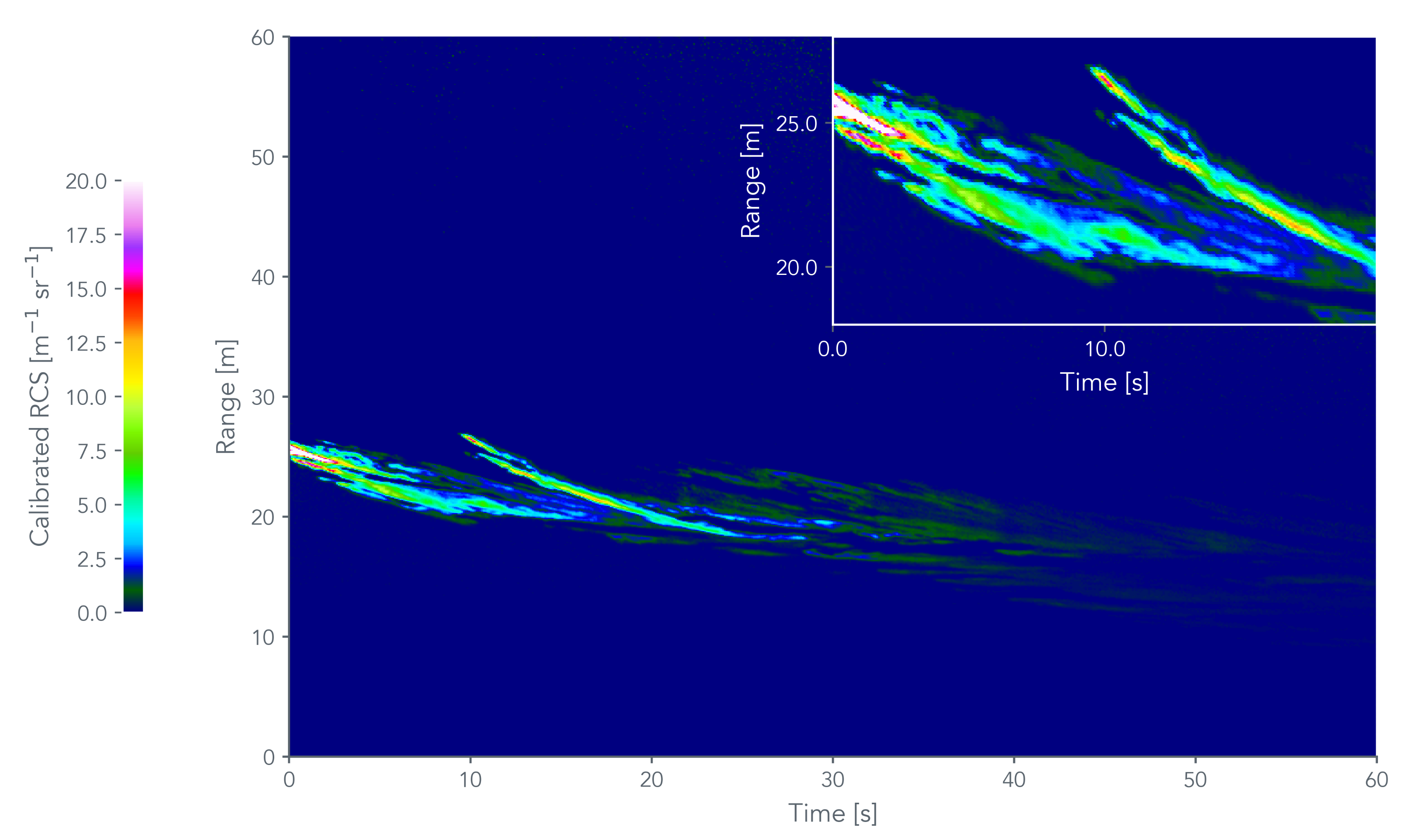
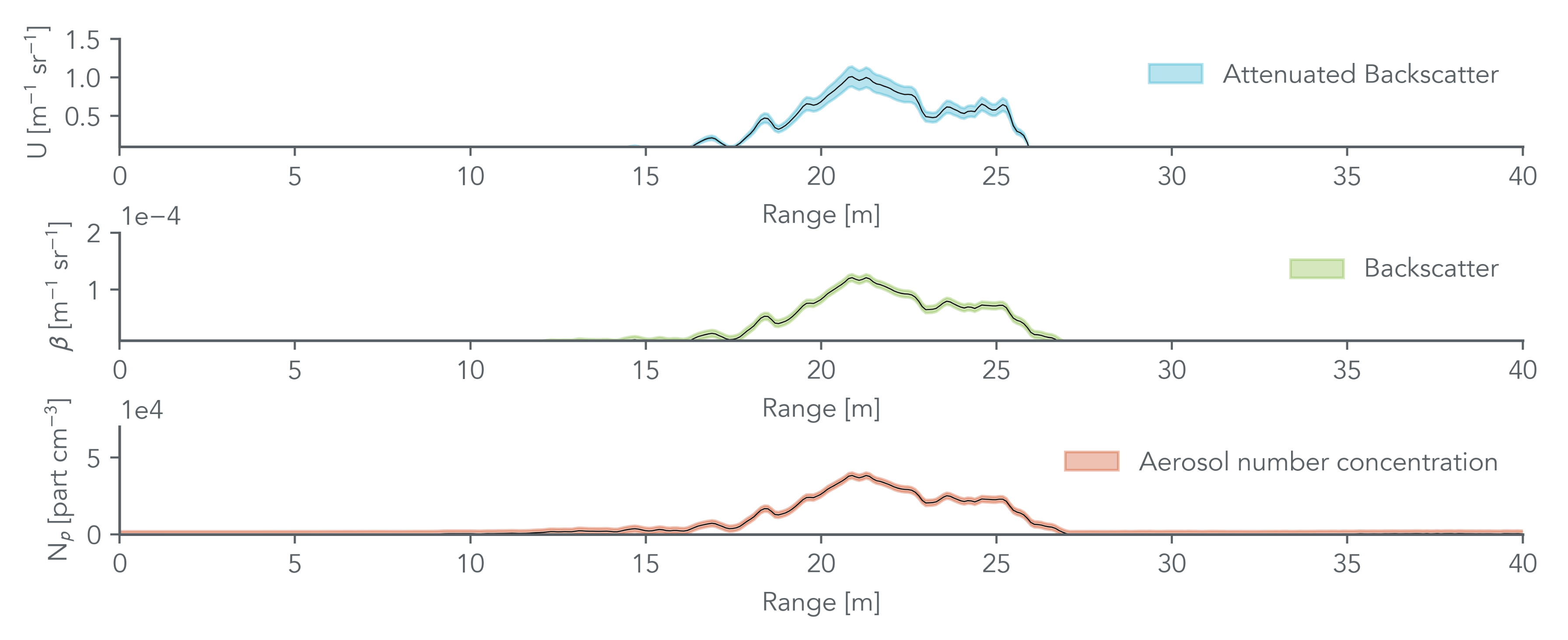
3.3. Attenuated Backscatter Profiles

One objective of the Colibri micro-lidar is to monitor the evolution and dispersion of the aerosol plumes, here fog-oil smoke particles, in the short-range with high range-resolution and temporal-resolution. Attenuated backscatter profiles $\mathrm{U}\left(\mathrm{r}\right)$ are the first-level micro-lidar products. They can be used to give a direct indication of the spatio-temporal distribution and structure of the aerosol plumes.

Figure 4 shows an example of the Colibri micro-lidar measurements carried out on 13th February at ONERA center. The glycol fog-oil emission event was remotely and horizontally characterized from 0 to 60 m during 60 s. It was possible to study the structural properties and spatio-temporal variability of the aerosol layers in the short-range with high range and temporal resolution. Note that all range levels given in this section are meant as the horizontal distance from the lidar system. The range-corrected signal RCS measurements were converted to attenuated backscatter profiles by applying the geometric and radiometric calibration procedure, fully explained in the previous Section 2.3.

A straightforward pre-processing procedure was employed to improve the quality of the lidar signals because of the high signal-to-noise ratio in the short-range and the fact that all measurements were done in an indoor environment. First, a 10 min measurement of dark current (DC) was done at the end measurement for each day during the campaign, covering the telescope (obtaining up to 100,000 profiles). DC measurements were first subtracted to the lidar signals. The background (BG) contribution was measured in the long-range (over 80 m). The BG presented a Gaussian distribution, therefore the mean value was used for suppressing the noise to each profile. Lastly, a 50 ms temporal-averaging filter was used to smooth the micro-lidar signals for the particle inversion method.

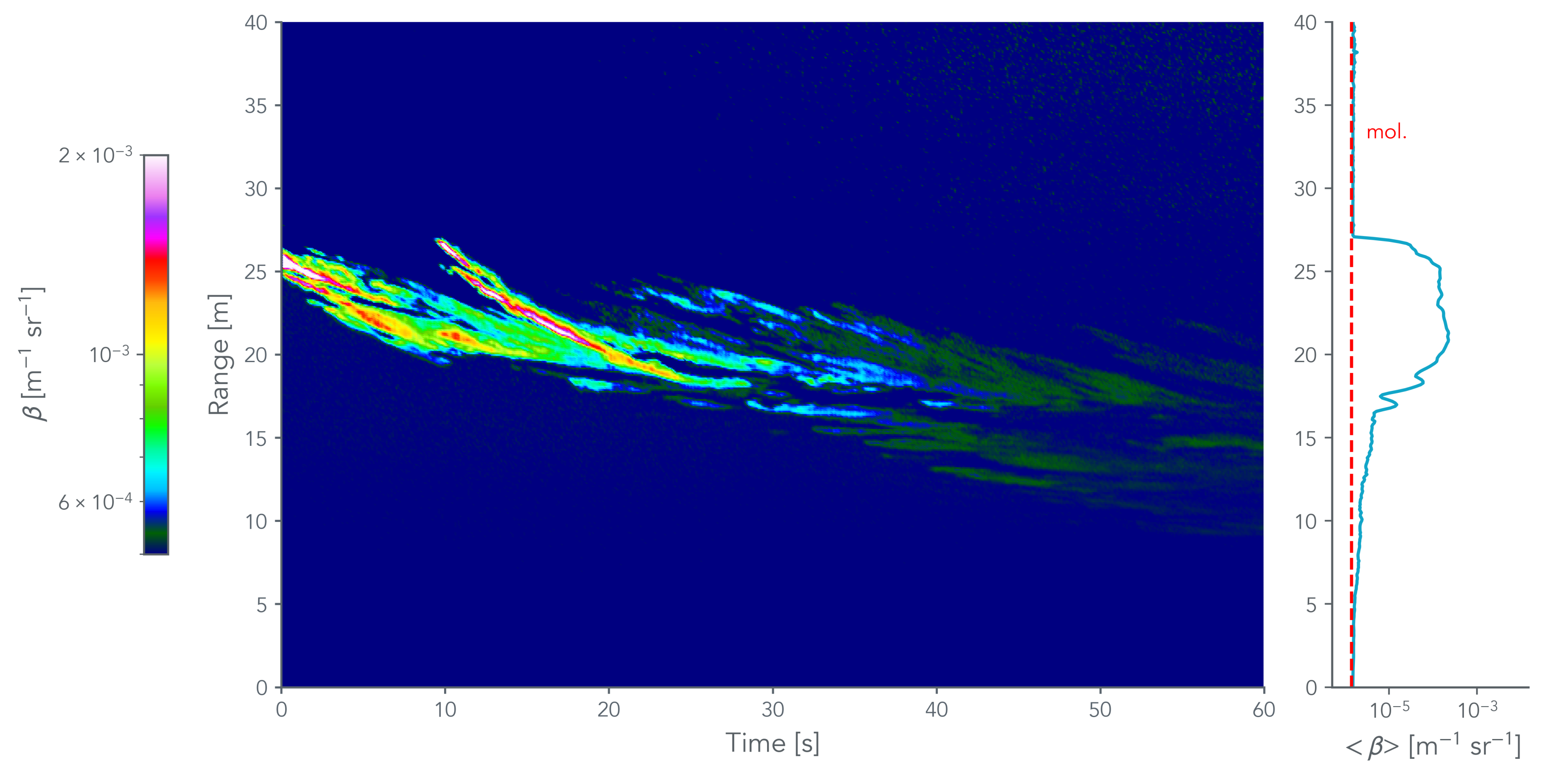
3.4. Aerosol Backscatter Profiles

The aerosol backscatter profiles ${\beta }_{\mathrm{aer}}\left(\mathrm{r}\right)$ are retrieved from the attenuated backscatter profiles according to the forward inverse method without boundary conditions presented in Section 2.4. The Lidar Ratio computed previously for fog-oil particles from light-scattering was specified for retrieving the aerosol backscatter lidar profiles.

Figure 5 presents the retrieved aerosol backscatter profiles of the fog-oil event in false color. In the studied case, the intense period of the event was centered from 20 to 28 m in the first 20 s of the measurement with averaged values for particle backscatter profiles close to those reported in the literature for such particles [15]. It should also be noted that the lowest detectable backscattering coefficients depend on signal and noise levels in the actual measurements. For detailed analysis, a comparison with the ambient molecular backscatter is proposed. The Rayleigh theory is used to compute the molecular backscatter coefficient with the height-scaled pressure at 20 °C and relative humidity ranging from 50 to 80% at the wavelength of interest, obtaining molecular backscatter coefficient values up to 4.25 ${10}^{-6}$ sr${}^{-1}$m${}^{-1}$. The right panel of Figure 5 presents the time-averaged (60 s) aerosol backscatter in blue color. For reference, the molecular backscatter profile is displayed in red. It is worth noting that the limit of detection for these measurements reaches the level of the molecular backscatter coefficient. This is evidencing the performances of the Colibri micro-lidar as well as the satisfactory implementation of the pre-processing and calibration methods.

Finally, the retrieved values of backscatter coefficients validate the effectiveness of the proposed forward inverse method without boundary conditions. The measured backscatter profiles demonstrate the system capability to characterize complex aerosol events in the short-range, close to their sources, with high range and temporal resolution. According to these first measurements, the Colibri micro-lidar is a good candidate to assess the dynamics of aerosol propagation in the short-range with millisecond temporal resolution. Further studies should be conducted to assess the system performances for vertical aerosol profiling in the atmosphere. The determination of the aerosol number concentration in the aerosol plume from micro-lidar profiles follows in the next section.

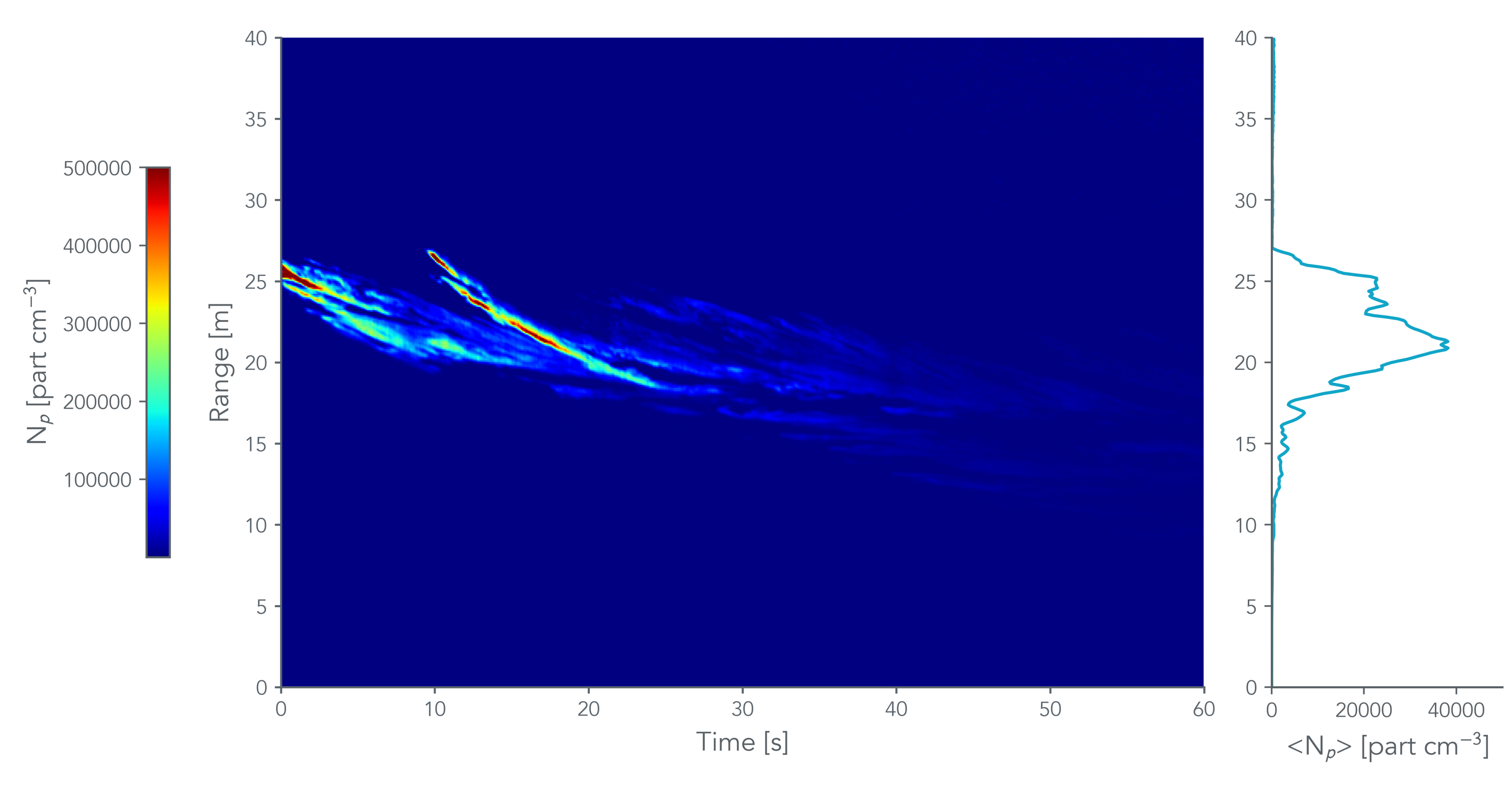
3.5. Number Concentration

The aerosol number concentration ${\mathrm{N}}_{\mathrm{p}}\left(\mathrm{r}\right)$ can be retrieved from aerosol backscatter signal using ancillary information provided by the optical particle counter (Fidas 200) and reported in Section 3.2. Following the same structure of the previous subsection, the backscatter profiles ${\beta }_{\mathrm{aer}}\left(\mathrm{r}\right)$ yield an estimation of the range-dependant aerosol number concentration ${\mathrm{N}}_{\mathrm{p}}\left(\mathrm{r}\right)$.

For a non-range dependant aerosol size distribution, let us write Equation (6) as:

$${\beta }_{\mathrm{aer}}\left(\mathrm{r}\right)={\mathrm{N}}_{\mathrm{p}}\left(\mathrm{r}\right)\langle \mathrm{d}{C}^{\mathrm{bac}}\rangle \left[m^{-1}s{r}^{-1}\right]$$

(23)

where $\langle \mathrm{d}{C}^{\mathrm{bac}}\rangle$ is the average differential backscattering cross-section calculated for the normalized fog-oil plume log-normal distribution. Thus, the number concentration can be estimated from he retrieved aerosol backscatter profiles as:

$${\mathrm{N}}_p\left(\mathrm{r}\right)=\frac{{\beta }_{\mathrm{aer}}\left(\mathrm{r}\right)}{\langle \mathrm{d}{C}^{\mathrm{bac}}\rangle }\left[\mathrm{part}{\mathrm{cm}}^{-3}\right]$$

(24)

Figure 6 shows the retrieved aerosol number concentration profiles of the fog-oil event in false color. From the measurements, a high number concentration of particles was detected in the first 30 s of the measurement, reaching values up to 5.0 ${10}^5$ part cm${}^{-3}$, and then evidencing the rapid decrease of the number of aerosol concentration over time, reaching values lower than ${10}^5$ part cm${}^{-3}$ in less than 30 s. The time-averaged aerosol number concentration $〈N_p〉$ measured during the first 60 s of the event is represented in the right panel of Figure 6.

4. Discussion

The major novelties of the Colibri micro-lidar lie in its ability to perform lidar measurements and retrieve quantitative aerosols products in the short-range, within the first hundreds of meters, and with high range and temporal resolution. The present section discusses several aspects relative to these novelties including: (i) a range and temporal resolution performance analysis, (ii) an error analysis based on calibration experimental errors, and (iii) a comparative analysis of aerosol products between lidar and optical counter.

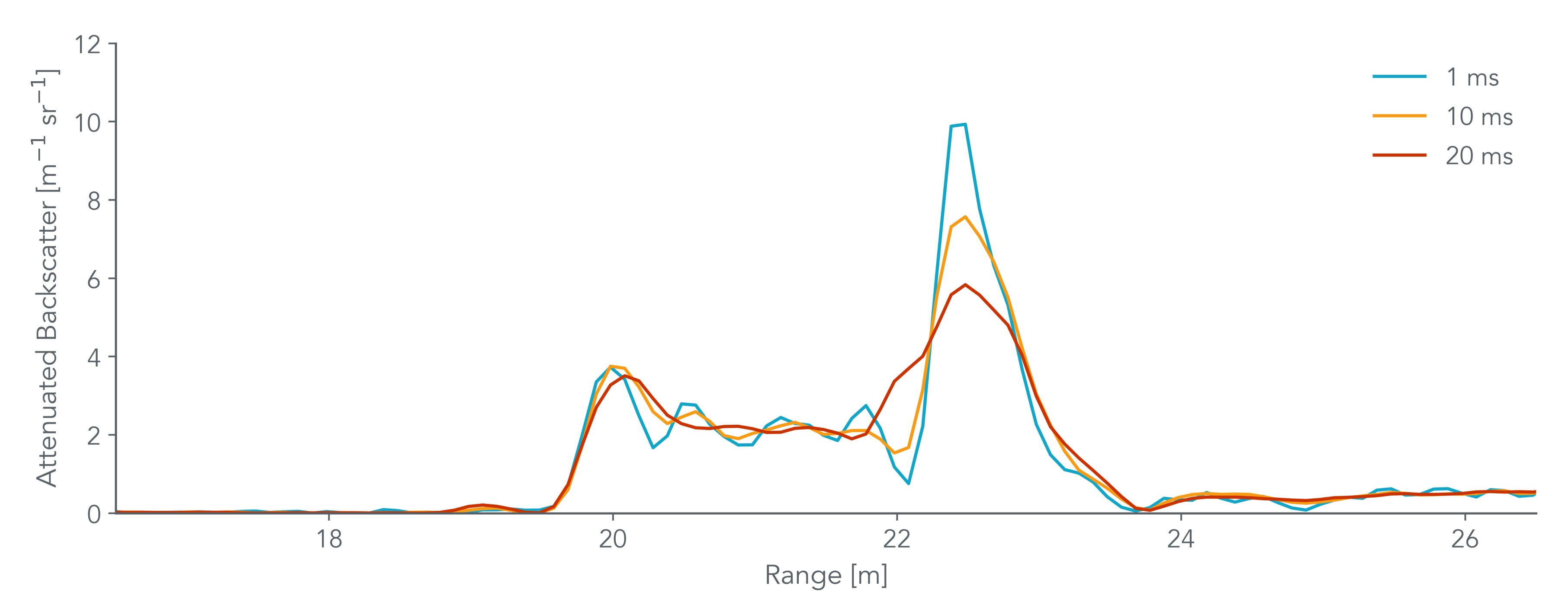
4.1. Range and Temporal Resolution Analysis

A fundamental difference between the Colibri micro-lidar and atmospheric elastic lidar systems lies in the achieved range and temporal resolution. Regarding the range resolution of the Colibri micro-lidar, the measurements in Section 3 were not range-averaged and the range resolution remains below 10 cm. No bin averaging technique was necessary and the range resolution is mainly limited by the laser pulse duration, the temporal response of the Si-APD, and the analog-to-digital converter bandwidth. Regarding the temporal resolution, the measurements in Section 3 were temporally-averaged and the temporal resolution remains at 10 cm.

In addition, the Colibri micro-lidar differs in terms of measurement times. Figure 7 displays single attenuated backscatter profiles at multiple time-resolution (1 ms, 10 ms, 20 ms) to highlight the capabilities of our instrument. While most of the atmospheric lidar systems usually provide time-integrated profiles over more than a few tens of seconds or minutes, the Colibri micro-lidar measures instantaneous aerosol lidar profiles with 1 ms time resolution (reduced to 50 ms after time-averaging to ease the signal processing).

While most elastic backscatter lidars usually cover a range resolution of tens of meters, the Colibri micro-lidar range and temporal resolution are 10 cm and 1 ms, respectively. These unique features will allow in the future to characterize fast aerosol events with a high temporal resolution with high range-resolution. For instance, problems such as new particle formation or secondary aerosol formation [57] involve rapid changes in aerosol particle size distribution, which are believed to play important roles for air quality assessment in urban and industrial areas. The study of such processes could greatly benefit from short-range elastic backscatter micro-lidar with high range and temporal resolution.

4.2. Uncertainty Analysis and Error Propagation

The quantification of lidar uncertainties by error propagation is necessary for evaluating the quality of retrieved lidar products such as aerosol backscatter or number concentration. The purpose here is to evaluate the error propagation during the fog-oil event. The uncertainties in the lidar products result from uncertainties in the pre-processing, i.e., DC and BG, and in the geometric and radiometric calibration, i.e., $\mathrm{O}\left(\mathrm{r}\right)$ and K${}_0^{*}$.

We assess in the following the total uncertainties by error propagation in the different lidar products presented along the manuscript, namely attenuated backscatter U(r), backscatter profiles ${\beta }_{\mathrm{aer}}\left(\mathrm{r}\right)$, and aerosol number concentration ${\mathrm{N}}_{\mathrm{p}}\left(\mathrm{r}\right)$. The noise of the variables is assumed uncorrelated, but the variables have a certain degree of dependency since calibration parameters were measured using the same instrumental setup. The measurements were not performed under the same exact experimental conditions (i.e., statistical and ambient changes could be considered over time); however, the use of the same Lambertian surface to retrieve the calibration parameters was found to be a stable and reliable method.

The lidar uncertainties are estimated by error propagation for instantaneous RCS profiles by deriving the Equations (15), (21) and (24), as

$$\delta \mathrm{RCS}(\mathrm{r})=\left[\frac{\delta \mathrm{DC}}{〈\mathrm{DC}〉}+\frac{\delta \mathrm{BG}}{〈\mathrm{BG}〉}\right]\mathrm{RCS}(\mathrm{r})$$

(25)

where $\delta \mathrm{DC}$ and $\delta \mathrm{BG}$ are the uncertainties associated to the pre-processing quantities DC and BG.

$$\delta \mathrm{U}(\mathrm{r})=\left[\frac{\delta \mathrm{RCS}}{〈\mathrm{RCS}〉}+\frac{\delta {\mathrm{K}}_{\mathrm{o}}^{*}}{〈{\mathrm{K}}_{\mathrm{o}}^{*}〉}+\frac{\delta \mathrm{O}\left(\mathrm{r}\right)}{〈\mathrm{O}\left(\mathrm{r}\right)〉}\right]\mathrm{U}(\mathrm{r})$$

(26)

$$\delta \beta \left(\mathrm{r}\right)=\left[\left(1+2\mathrm{LR}\beta \left(\mathrm{r}\right)\mathrm{U}\left(\mathrm{r}\right)/\mathrm{U}’\left(\mathrm{r}\right)\right)\frac{\delta \mathrm{U}\left(\mathrm{r}\right)}{\mathrm{U}\left(\mathrm{r}\right)}\right]\beta \left(\mathrm{r}\right)$$

(27)

$$\delta {\mathrm{N}}_p\left(\mathrm{r}\right)=\left[\frac{\delta \beta \left(\mathrm{r}\right)}{\beta }\right]{\mathrm{N}}_p\left(\mathrm{r}\right)$$

(28)

where $\delta {\mathrm{K}}_{\mathrm{o}}^{*}$ and $\delta \mathrm{O}\left(\mathrm{r}\right)$ are the uncertainties associated to the calibration quantities ${\mathrm{K}}_{\mathrm{o}}^{*}$ and $\mathrm{O}\left(\mathrm{r}\right)$. The fact that Equation (27) has a derivative term in the denominator may drive to some singularities in the $\delta \beta$ calculation, but in any case can not be associated as error propagation of ${\mathrm{K}}_{\mathrm{o}}^{*}$ or $\mathrm{O}\left(\mathrm{r}\right)$ over $\beta (\mathrm{r}$) or ${\mathrm{N}}_p\left(\mathrm{r}\right)$.

Figure 8 summarizes the error propagation results for typical micro-lidar products from Section 3. As a result, the total error propagation over $\beta \left(\mathrm{r}\right)$ and ${\mathrm{N}}_p\left(\mathrm{r}\right)$, considering both the pre-processing and calibration, leads to consider a mean relative mean error lower than 14%. This error analysis yields a significant insight into the robustness of the proposed calibration method for retrieving aerosol products in the short-range using the Colibri micro-lidar.

4.3. Comparative Analysis with Local Sensors

In the following, we propose a comparative analysis between the aerosol number concentration retrieved from the Colibri and Fidas 200 during the fog-oil event. The objective is to validate the proposed methodology for short-range micro-lidar. Prior to the comparison, we should recall the different nature of the two instruments. Elastic backscatter lidars are remote-sensing instruments that provide range-dependant aerosol products whereas optical particle counters are local sensors that measure aerosols properties (e.g., particle size distribution, particle concentration) in a single location. The direct products of the Fidas 200 are the particle matter concentrations (PM1, PM2.5, PM10) at relatively high temporal resolution (1s), nevertheless, elaborated products such as particle and mass concentration are time-integrated products. Considering that, both instruments will measure the fog-oil event, but Fidas 200 is retrieving the particle number concentration as a function of the diameter for the air column where Fidas 200 is located (4 m away to the fog-oil generator and about 25 m from the micro-lidar). Meanwhile, the aerosol number concentration retrieved from the Colibri micro-lidar measurements are provided with a native spatio-temporal resolution for a scattering-volume along the tunnel.

To use the Fidas 200 product as a reference during the event, comparable products should be computed for both instruments in order to preserve their principle of the measurement. The temporal mean of the N${}_p$ is calculated here and is directly provided by the Fidas 200. For the Colibri micro-lidar, a range and temporal mean was performed around the fog-oil plume from 0 to 40 m and from 0 to 60 s. This makes it possible to carry out a comparison in

Table 3. Range and 60 s time-averaged aerosol number concentration $〈N_p〉$ derived from the Colibri micro-lidar and aerosol number concentration from Fidas 200 optical counter.

Averaged Aerosol Number Concentration
Instrument	Value	Units
Colibri	3990 ± 130	part cm${}^{-3}$
Fidas 200	4055 ± 400	part cm${}^{-3}$

between the mean values retrieved from both instruments.

Table 3 presents the time and range-averaged aerosol number concentration from the Colibri and Fidas 200 instruments $<{\mathrm{N}}_p>=4350$ part cm${}^{-3}$ and $<{\mathrm{N}}_p>=3990$ part cm${}^{-3}$ respectively. This comparison yields a good agreement between the Colibri micro-lidar and the Fidas 200. The differences might be associated on the one hand to the different nature of the instrument: while the Colibri micro-lidar is a remote-sensing instrument that measures range-resolved number concentration of particles, Fidas 200 is an in-situ instrument that performs measurements from a single location. On the other hand, the differences in temporal resolution between instruments might yield erroneous results, considering that Fidas 200 reported less than 15 measurements during the fog-oil event, which is far from being directly comparable with the millisecond temporal resolution of the Colibri micro-lidar. Finally, this analysis assesses the performances of the Colibri micro-lidar for providing quantitive number concentration profiles for complex aerosol events in the short-range, close to their sources, and with high range-resolution and high temporal-resolution.

5. Conclusions

The present work has demonstrated the feasibility of our self-designed short-range elastic backscatter micro-lidar to provide relevant properties of aerosol plumes, including radiative and microphysical properties. An indoor measurement campaign was carried out to assess the performances of the micro-lidar under controlled environment conditions. This campaign allowed us to monitor the dynamics of aerosol plumes and to retrieve quantitative micro-lidar products, including aerosol backscatter and number concentration profiles as a result of a rigorous calibration and a dedicated inverse method without any boundary condition. In a nutshell, the following highlights can be drawn from our in-door measurement campaign using the Colibri micro-lidar:

(i)

Short-range elastic backscatter lidar measurements were proved to measure backscattering from aerosol plumes in the short-range (within the first tens of meters) with a high range-resolution (<10 cm) and a high-temporal-resolution (1 ms);

(ii)

The inversion of micro-lidar signals was made possible using a forward inverse method without boundary conditions;

(iii)

Aerosol backscatter and number concentration profiles could be retrieved using lidar-relevant parameters derived from light-scattering models and ancillary in-situ instruments.

The Colibri micro-lidar fills technological gaps (i.e., high range-resolution, short-range) that current elastic lidar systems have not yet covered. Such high-resolution could enable lidar measurements of small aerosol plumes or rapidly changing aerosol events. For instance, it could enable the study of radiative and microphysical properties of aerosols associated with complex atmospheric processes such as new particle formation (i.e., nucleation process) and aerosol dynamics inside the atmospheric boundary layer, and also for the characterization of the emitting sources in industrial and aeronautics sectors. These aerosol lidar products are currently necessary for different atmospheric research and industrial fields. Furthermore, it is worth noting that the aerosol plume was never in contact with our system, which supports the potential use of this system for standoff sensing of particulate matter such as hazardous industrial plumes or aerosolized bioagent for instance.

For transferring the Colibri micro-lidar from indoor tunnel measurements to outdoor field campaigns, the current prototype should undergo a series of adjustments, including an adaptation of interference filter and spatial filter to improve the rejection of ambient background light and optimize the signal-to-noise ratio. Moreover, a challenge in aerosol lidar has been for many years to rigorously account for the validity of the single-scattering approximation. To improve the quality of micro-lidar retrievals for dense aerosol plumes, the relative contribution of multiple-scattering should be evaluated in the future, and additionally, the instrument is planned to be extended to multi-wavelength operation in order to retrieve high-level products such as high spatio-temporal Angstrom Exponent and color ratio products in order to go further at investigating complex topics such as aerosol-cloud interaction (i.e., inside the Atmospheric Boundary Layer Cirrus clouds and fog formation near to the surface), which are essentials for the Earth’s radiative balance calculations and atmospheric modeling. Additionally, our results suggest the implementation of new aerosol field campaigns for having a long-term database of aerosol properties. Taking advantage of the high range and temporal resolution measurements, new particle formation and near real-time aerosol dynamics of such processes could be addressed in the future. This will give us the possibility to explore new light-scattering problems related to lidar technologies.

References

- Liu, Z.; Omar, A.; Vaughan, M.; Hair, J.; Kittaka, C.; Hu, Y.; Powell, K.; Trepte, C.; Winker, D.; Hostetler, C.; et al. CALIPSO lidar observations of the optical properties of Saharan dust: A case study of long-range transport. J. Geophys. Res. Atmos. 2008, 113. [Google Scholar] [CrossRef]
- Sicard, M.; Molero, F.; Guerrero-Rascado, J.L.; Pedros, R.; Exposito, F.J.; Cordoba-Jabonero, C.; Bolarin, J.M.; Comeron, A.; Rocadenbosch, F.; Pujadas, M.; et al. Aerosol Lidar Intercomparison in the Framework of SPALINET—The Spanish Lidar Network: Methodology and Results. IEEE Trans. Geosci. Remote Sens. 2009, 47, 3547–3559. [Google Scholar] [CrossRef]
- Burton, S.P.; Ferrare, R.A.; Hostetler, C.A.; Hair, J.W.; Rogers, R.R.; Obland, M.D.; Butler, C.F.; Cook, A.L.; Harper, D.B.; Froyd, K.D. Aerosol classification using airborne High Spectral Resolution Lidar measurements—Methodology and examples. Atmos. Meas. Tech. 2012, 5, 73–98. [Google Scholar] [CrossRef]
- Pappalardo, G.; Amodeo, A.; Pandolfi, M.; Wandinger, U.; Ansmann, A.; Bösenberg, J.; Matthias, V.; Amiridis, V.; Tomasi, F.D.; Frioud, M.; et al. Aerosol lidar intercomparison in the framework of the EARLINET project. 3. Ramanlidar algorithm for aerosol extinction, backscatter, and lidar ratio. Appl. Opt. 2004, 43, 5370–5385. [Google Scholar] [CrossRef]
- Brown, A.J.; Videen, G.; Zubko, E.; Heavens, N.; Schlegel, N.J.; Beccera, P.; Meyer, C.; Harrison, T.; Hayne, P.; Obbard, R.; et al. The case for a multi-channel polarization sensitive LIDAR for investigation of insolation-driven ices and atmospheres Planetary Science Decadal Survey White Paper. Earth Space Sci. Open Arch. 2020. [Google Scholar] [CrossRef]
- Welton, E.J.; Campbell, J.R. Micropulse Lidar Signals: Uncertainty Analysis. J. Atmos. Ocean. Technol. 2002, 19, 2089–2094. [Google Scholar] [CrossRef]
- Gong, W.; Li, J.; Mao, F.; Zhang, J. Comparison of simultaneous signals obtained from a dual-field-of-view lidar and its application to noise reduction based on empirical mode decomposition. Chin. Opt. Lett. 2011, 9, 050101. [Google Scholar] [CrossRef]
- Ong, P.M.; Lagrosas, N.; Shiina, T.; Kuze, H. Surface Aerosol Properties Studied Using a Near-Horizontal Lidar. Atmosphere 2019, 11, 36. [Google Scholar] [CrossRef]
- Edner, H.; Ragnarson, P.; Wallinder, E. Industrial Emission Control Using Lidar Techniques. Environ. Sci. Technol. 1995, 29, 330–337. [Google Scholar] [CrossRef]
- Guerrero-Rascado, J.L.; da Costa, R.F.; Bedoya, A.E.; Guardani, R.; Alados-Arboledas, L.; Álvaro, E.B.; Landulfo, E. Multispectral elastic scanning lidar for industrial flare research: Characterizing the electronic subsystem and application. Opt. Express 2014, 22, 31063–31077. [Google Scholar] [CrossRef]
- Del Guasta, M. Daily cycles in urban aerosols observed in Florence (Italy) by means of an automatic 532–1064nm LIDAR. Atmos. Environ. 2002, 36, 2853–2865. [Google Scholar] [CrossRef]
- Schröter, M.; Obermeier, A.; Brüggemann, D.; Plechschmidt, M.; Klemm, O. Remote Monitoring of Air Pollutant Emissions from Point Sources by a Mobile Lidar/Sodar System. J. Air Waste Manag. Assoc. 2003, 53, 716–723. [Google Scholar] [CrossRef] [PubMed][Green Version]
- De Arruda Moreira, G.; Guerrero-Rascado, J.L.; Benavent-Oltra, J.A.; Ortiz-Amezcua, P.; Román, R.; Bedoya-Velásquez, A.E.; Bravo-Aranda, J.A.; Olmo Reyes, F.J.; Landulfo, E.; Alados-Arboledas, L. Analyzing the turbulent planetary boundary layer by remote sensing systems: The Doppler wind lidar, aerosol elastic lidar and microwave radiometer. Atmos. Chem. Phys. 2019, 19, 1263–1280. [Google Scholar] [CrossRef]
- Evgenieva, T.T.; Kolev, N.I.; Iliev, I.T.; Savov, P.B.; Kaprielov, B.K.; Devara, P.C.S.; Kolev, I.N. Lidar and spectroradiometer measurements of atmospheric aerosol optical characteristics over an urban area in Sofia, Bulgaria. Int. J. Remote Sens. 2009, 30, 6381–6401. [Google Scholar] [CrossRef]
- Giles, J.W.; Bankman, I.N.; Sova, R.M.; Morgan, T.R.; Duncan, D.D.; Millard, J.A.; Green, W.J.; Marcotte, F.J. Lidar system model for use with path obscurants and experimental validation. Appl. Opt. 2008, 47, 4085–4093. [Google Scholar] [CrossRef]
- Tremblay, G.; Cao, X.; Roy, G. The effect of dense aerosol cloud on the 3D information contain of flash Lidar. Proc. SPIE Int. Soc. Opt. Eng. 2010, 7828. [Google Scholar] [CrossRef]
- Brown, D.M.; Thrush, E.; Thomas, M.E. Chamber lidar measurements of biological aerosols. Appl. Opt. 2011, 50, 717–724. [Google Scholar] [CrossRef]
- Brown, D.M.; Brown, A.M.; Willitsford, A.H.; Dinello-Fass, R.; Airola, M.B.; Siegrist, K.M.; Thomas, M.E.; Chang, Y. Lidar measurements of solid rocket propellant fire particle plumes. Appl. Opt. 2016, 55, 4657–4669. [Google Scholar] [CrossRef]
- Kleiman, M.M.; Shiloah, N. Effect of dense atmospheric environment on the performance of laser radar sensors used for collision avoidance. Proc. SPIE 1999, 3707, 624–635. [Google Scholar] [CrossRef]
- Song, W.; Lai, J.; Ghassemlooy, Z.; Gu, Z.; Yan, W.; Wang, C.; Li, Z. The effect of fog on the probability density distribution of the ranging data of imaging laser radar. AIP Adv. 2018, 8, 025022. [Google Scholar] [CrossRef]
- Cao, X.; Church, P.; Matheson, J.; Roy, G. Optimization of obscurant penetration with next generation lidar technology. Proc. SPIE 2019, 11005, 217–228. [Google Scholar]
- Bissonnette, L.R. Lidar and Multiple Scattering. In Lidar: Range-Resolved Optical Remote Sensing of the Atmosphere; Springer New York: New York, NY, USA, 2005; pp. 43–103. [Google Scholar] [CrossRef]
- Mishchenko, M.I.; Travis, L.D.; Lacis, A.A. Scattering, Absorption, and Emission of Light by Small Particles; Cambridge University Press: Cambridge, UK, 2002. [Google Scholar]
- Berg, M.J.; Sorensen, C.M.; Chakrabarti, A. Extinction and the optical theorem. Part I. Single particles. J. Opt. Soc. Am. A 2008, 25, 1504–1513. [Google Scholar] [CrossRef] [PubMed]
- Fernald, F.G.; Herman, B.M.; Reagan, J.A. Determination of aerosol height distributions by lidar. J. Appl. Meteorol. 1972, 11, 482–489. [Google Scholar] [CrossRef]
- Klett, J.D. Stable analytical inversion solution for processing lidar returns. Appl. Opt. 1981, 20, 211–220. [Google Scholar] [CrossRef] [PubMed]
- Fernald, F.G. Analysis of atmospheric lidar observations: Some comments. Appl. Opt. 1984, 23, 652–653. [Google Scholar] [CrossRef] [PubMed]
- Anderson, T.; Covert, D.; Wheeler, J.; Harris, J.; Perry, K.; Trost, B.; Jaffe, D.; Ogren, J. Aerosol backscatter fraction and single scattering albedo: Measured values and uncertainties at a coastal station in the Pacific Northwest. J. Geophys. Res. Atmos. 1999, 104, 26793–26807. [Google Scholar] [CrossRef]
- Cattrall, C.; Reagan, J.; Thome, K.; Dubovik, O. Variability of aerosol and spectral lidar and backscatter and extinction ratios of key aerosol types derived from selected Aerosol Robotic Network locations. J. Geophys. Res. Atmos. 2005, 110. [Google Scholar] [CrossRef]
- Müller, D.; Ansmann, A.; Mattis, I.; Tesche, M.; Wandinger, U.; Althausen, D.; Pisani, G. Aerosol-type-dependent lidar ratios observed with Raman lidar. J. Geophys. Res. Atmos. 2007, 112. [Google Scholar] [CrossRef]
- Barnaba, F.; Gobbi, G.P. Modeling the aerosol extinction versus backscatter relationship for lidar applications: Maritime and continental conditions. J. Atmos. Ocean. Technol. 2004, 21, 428–442. [Google Scholar] [CrossRef]
- Paulien, L.; Ceolato, R.; Soucasse, L.; Enguehard, F.; Soufiani, A. Lidar-relevant radiative properties of soot fractal aggregate ensembles. J. Quant. Spectrosc. Radiat. Transf. 2020, 241, 106706. [Google Scholar] [CrossRef]
- Kanngiesser, F.; Kahnert, M. Coating material-dependent differences in modelled lidar-measurable quantities for heavily coated soot particles. Opt. Express 2019, 27, 36368–36387. [Google Scholar] [CrossRef] [PubMed]
- Ceolato, R.; Paulien, L.; Maughan, J.B.; Sorensen, C.M.; Berg, M.J. Radiative properties of soot fractal superaggregates including backscattering and depolarization. J. Quant. Spectrosc. Radiat. Transf. 2020, 247, 106940. [Google Scholar] [CrossRef]
- Zuev, V. Laser Beams in the Atmosphere; Wood, J., Ed.; Consultants Bureau: New York, NY, USA, 1982; Available online: https://www.springer.com/gp/book/9781468488838 (accessed on 23 September 2020).
- Measures, R.M. Laser Remote Sensing: Fundamentals and Applications; Wiley-Interscience: New York, NY, USA, 1984. [Google Scholar]
- Kavaya, M.J.; Menzies, R.T.; Haner, D.A.; Oppenheim, U.P.; Flamant, P.H. Target reflectance measurements for calibration of lidar atmospheric backscatter data. Appl. Opt. 1983, 22, 2619–2628. [Google Scholar] [CrossRef]
- Halldórsson, T.; Langerholc, J. Geometrical form factors for the lidar function. Appl. Opt. 1978, 17. [Google Scholar] [CrossRef] [PubMed]
- Harms, J. Lidar return signals for coaxial and noncoaxial systems with central obstruction. Appl. Opt. 1979, 18, 1559–1566. [Google Scholar] [CrossRef]
- Sasano, Y.; Shimizu, H.; Takeuchi, N.; Okuda, M. Geometrical form factor in the laser radar equation: An experimental determination. Appl. Opt. 1979, 18, 3908–3910. [Google Scholar] [CrossRef]
- Dho, S.W.; Park, Y.J.; Kong, H.J. Experimental determination of a geometric form factor in a lidar equation for an inhomogeneous atmosphere. Appl. Opt. 1997, 36. [Google Scholar] [CrossRef]
- Wandinger, U.; Ansmann, A. Experimental determination of the lidar overlap profile with Raman lidar. Appl. Opt. 2002, 41. [Google Scholar] [CrossRef]
- Guerrero-Rascado, J.L.; Costa, M.J.; Bortoli, D.; Silva, A.M.; Lyamani, H.; Alados-Arboledas, L. Infrared lidar overlap function: An experimental determination. Opt Express 2010, 18, 20350–20359. [Google Scholar] [CrossRef]
- Vande Hey, J.; Coupland, J.; Foo, M.H.; Richards, J.; Sandford, A. Determination of overlap in lidar systems. Appl. Opt. 2011, 50, 5791–5797. [Google Scholar] [CrossRef]
- Biavati, G.; Di Donfrancesco, G.; Cairo, F.; Feist, D.G. Correction scheme for close-range lidar returns. Appl. Opt. 2011, 50, 5872–5882. [Google Scholar] [CrossRef] [PubMed]
- Li, J.; Li, C.; Zhao, Y.; Li, J.; Chu, Y. Geometrical constraint experimental determination of Raman lidar overlap profile. Appl. Opt. 2016, 55, 4924–4928. [Google Scholar] [CrossRef] [PubMed]
- Stelmaszczyk, K.; Dell’Aglio, M.; Chudzyński, S.; Stacewicz, T.; Wöste, L. Analytical function for lidar geometrical compression form-factor calculations. Appl. Opt. 2005, 44, 1323–1331. [Google Scholar] [CrossRef] [PubMed]
- Ceolato, R.; Riviere, N.; Hespel, L. Reflectances from a supercontinuum laser-based instrument: Hyperspectral, polarimetric and angular measurements. Opt. Express 2012, 20, 29413–29425. [Google Scholar] [CrossRef] [PubMed]
- Wagner, W.; Ullrich, A.; Ducic, V.; Melzer, T.; Studnicka, N. Gaussian decomposition and calibration of a novel small-footprint full-waveform digitising airborne laser scanner. ISPRS J. Photogramm. Remote Sens. 2006, 60, 100–112. [Google Scholar] [CrossRef]
- Chauve, A.; Vega, C.; Durrieu, S.; Bretar, F.; Allouis, T.; Deseilligny, M.P.; Puech, W. Advanced full-waveform lidar data echo detection: Assessing quality of derived terrain and tree height models in an alpine coniferous forest. Int. J. Remote Sens. 2009, 30, 5211–5228. [Google Scholar] [CrossRef]
- Shen, X.; Li, Q.Q.; Wu, G.; Zhu, J. Decomposition of LiDAR waveforms by B-spline-based modeling. ISPRS J. Photogramm. Remote Sens. 2017, 128, 182–191. [Google Scholar] [CrossRef]
- Palmer, W. Exposure Standard for Fog Oil; Technical Report; U.S. Army Biomedical Research and Development Laboratory: Fort Detrick, MD, USA, 1990; Volume 9010. Available online: https://www.osti.gov/biblio/5668868-exposure-standard-fog-oil-technical-report-dec-nov (accessed on 23 September 2020).
- Wieslander, G.; Norbäck, D.; Lindgren, T. Experimental exposure to propylene glycol mist in aviation emergency training: Acute ocular and respiratory effects. Occup. Environ. Med. 2001, 58, 649–655. [Google Scholar] [CrossRef]
- Mie, G. Beiträge zur Optik trüber Medien, speziell kolloidaler Metallösungen. Annalen der Physik 1908, 330, 377–445. [Google Scholar] [CrossRef]
- Yue, G.K.; Deepak, A. Modeling of coagulation-sedimentation effects on transmission of visible/IR laser beams in aerosol media. Appl. Opt. 1979, 18, 3918–3925. [Google Scholar] [CrossRef]
- Farmer, W.M.; Morris, R.D.; Schwartz, F.A. Optical particle size measurements of hygroscopic smokes inlaboratory and field environments. Appl. Opt. 1981, 20, 3929–3940. [Google Scholar] [CrossRef] [PubMed]
- Pan, X.; Kanaya, Y.; Taketani, F.; Miyakawa, T.; Inomata, S.; Komazaki, Y.; Tanimoto, H.; Wang, Z.; Uno, I.; Wang, Z. Emission characteristics of refractory black carbon aerosols from fresh biomass burning: Aperspective from laboratory experiments. Atmos. Chem. Phys. 2017, 17, 13001–13016. [Google Scholar] [CrossRef]