Summer Mass Balance and Surface Velocity Derived by Unmanned Aerial Vehicle on Debris-Covered Region of Baishui River Glacier No. 1, Yulong Snow Mountain


Abstract
1. Introduction
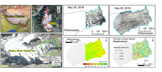
2. Study Area
3. Data and Method
3.1. Unmanned Aerial Vehicle
3.2. Flight Description
3.3. Ground Control Points
3.4. Orthomosaic and DEM Generation
3.5. COSI-Corr for Glacier Velocity
4. Results
4.1. Accuracy of DEMs and Orthomosaics
4.2. Orthomosaic and Digital Elevation Model
4.3. Mass Balance of Debris-Covered Glacier
4.4. Summer Surface Velocity
5. Discussion
5.1. Accuracy of DEMs and Orthomosaics
5.2. Changes in the Elevation and Mass Balance
5.3. Glacier Surface Velocity
5.4. Advantages and Disadvantages of the UAV Monitoring
6. Conclusions
Author Contributions
Funding
Acknowledgments
Conflicts of Interest
References
- Immerzeel, W.W.; van Beek, L.P.H.; Bierkens, M.F.P. Climate Change Will Affect the Asian Water Towers. Sciences 2010, 328, 1382–1385. [Google Scholar] [CrossRef]
- Immerzeel, W.W.; Lutz, A.F.; Andrade, M.; Bahl, A.; Biemans, H.; Bolch, T.; Hyde, S.; Brumby, S.; Davies, B.J.; Elmore, A.C.; et al. Importance and Vulnerability of the World’s Water Towers. Nature 2020, 577, 364–369. [Google Scholar] [CrossRef] [PubMed]
- Yao, T.; Wu, G.; Xu, B.; Wang, W.; Gao, J.; An, B. Asian Water Tower Change and Its Impacts. Bull. Chin. Acad. Sci. 2019, 34, 1203–1209. [Google Scholar]
- Farinotti, D. Cryospheric Science: Asia’s Glacier Changes. Nat. Geosci. 2017, 10, 621–622. [Google Scholar] [CrossRef]
- Usami, N.; Muhuri, A.; Bhattacharya, A.; Hirose, A. Proposal of Wet Snowmapping with Focus on Incident Angle Influential to Depolarization of Surface Scattering. In Proceedings of the 2016 IEEE International Geoscience and Remote Sensing Symposium (IGARSS), Beijing, China, 10–15 July 2016. [Google Scholar]
- Shean, D.E.; Bhushan, S.; Montesano, P.; Rounce, D.R.; Arendt, A.; Osmanoglu, B. A Systematic, Regional Assessment of High Mountain Asia Glacier Mass Balance. Front. Earth Sci. 2020, 7, 363. [Google Scholar] [CrossRef]
- Zhou, Y.; Li, Z.; Li, J.; Zhao, R.; Ding, X. Glacier Mass Balance in the Qinghai–Tibet Plateau and Its Surroundings from the Mid-1970s to 2000 Based on Hexagon Kh-9 and Srtm Dems. Remote Sens. Environ. 2018, 210, 96–112. [Google Scholar] [CrossRef]
- Paul, F.; Bolch, T.; Kääb, A.; Nagler, T.; Nuth, C.; Scharrer, K.; Shepherd, A.; Strozzi, T.; Ticconi, F.; Bhambri, R.; et al. The Glaciers Climate Change Initiative: Methods for Creating Glacier Area, Elevation Change and Velocity Products. Remote Sens. Environ. 2015, 162, 408–426. [Google Scholar] [CrossRef]
- Immerzeel, W.W.; Kraaijenbrink, P.D.A.; Shea, J.M.; Shrestha, A.B.; Pellicciotti, F.; Bierkens, M.F.P.; de Jong, S.M. High-Resolution Monitoring of Himalayan Glacier Dynamics Using Unmanned Aerial Vehicles. Remote Sens. Environ. 2014, 150, 93–103. [Google Scholar] [CrossRef]
- Arnold, N.S.; Rees, W.G.; Devereux, B.J.; Amable, G.S. Evaluating the Potential of High-Resolution Airborne Lidar Data in Glaciology. Int. J. Remote Sens. 2006, 27, 1233–1251. [Google Scholar] [CrossRef]
- Robson, B.A.; Nuth, C.; Dahl, S.O.; Hölbling, D.; Strozzi, T.; Nielsen, P.R. Automated Classification of Debris-Covered Glaciers Combining Optical, Sar and Topographic Data in an Object-Based Environment. Remote Sens. Environ. 2015, 170, 372–387. [Google Scholar] [CrossRef]
- Kaab, A.; Berthier, E.; Nuth, C.; Gardelle, J.; Arnaud, Y. Contrasting Patterns of Early Twenty-First-Century Glacier Mass Change in the Himalayas. Nature 2012, 488, 495–498. [Google Scholar] [CrossRef] [PubMed]
- Brun, F.; Berthier, E.; Wagnon, P.; Kaab, A.; Treichler, D. A Spatially Resolved Estimate of High Mountain Asia Glacier Mass Balances from 2000 to 2016. Nat. Geosci. 2017, 10, 668–673. [Google Scholar] [CrossRef] [PubMed]
- Maurer, J.M.; Schaefer, J.M.; Rupper, S.; Corley, A. Acceleration of Ice Loss across the Himalayas over the Past 40 Years. Sci. Adv. 2019, 5, eaav7266. [Google Scholar] [CrossRef] [PubMed]
- Rignot, E.; Kanagaratnam, P. Changes in the Velocity Structure of the Greenland Ice Sheet. Sciences 2006, 311, 986–990. [Google Scholar] [CrossRef] [PubMed]
- Li, T.; Liu, Y.; Li, T.; Hui, F.; Chen, Z.; Cheng, X. Antarctic Surface Ice Velocity Retrieval from Modis-Based Mosaic of Antarctica (Moa). Remote Sens. 2018, 10, 1045. [Google Scholar] [CrossRef]
- Fahnestock, M.; Scambos, T.; Moon, T.; Gardner, A.; Haran, T.; Klinger, M. Rapid Large-Area Mapping of Ice Flow Using Landsat 8. Remote Sens. Environ. 2016, 185, 84–94. [Google Scholar] [CrossRef]
- Scherler, D.; Bookhagen, B.; Strecker, M.R. Spatially Variable Response of Himalayan Glaciers to Climate Change Affected by Debris Cover. Nat. Geosci. 2011, 4, 156–159. [Google Scholar] [CrossRef]
- Gardelle, J.; Berthier, E.; Arnaud, Y.; Kaab, A. Region-Wide Glacier Mass Balances over the Pamir-Karakoram-Himalaya during 1999–2011. Cryosphere 2013, 7, 1885–1886. [Google Scholar] [CrossRef]
- Kraaijenbrink, P.D.A.; Bierkens, M.F.P.; Lutz, A.F.; Immerzeel, W.W. Impact of a Global Temperature Rise of 1.5 Degrees Celsius on Asia’s Glaciers. Nature 2017, 549, 257–260. [Google Scholar] [CrossRef]
- Kraaijenbrink, P.D.A.; Shea, J.M.; Litt, M.; Steiner, J.F.; Treichler, D.; Koch, I.; Immerzeel, W.W. Mapping Surface Temperatures on a Debris-Covered Glacier with an Unmanned Aerial Vehicle. Front. Earth Sci. 2018, 6, 64. [Google Scholar] [CrossRef]
- Wang, S.; Che, Y.; Pang, H.; Du, J.; Zhang, Z. Accelerated Changes of Glaciers in the Yulong Snow Mountain, Southeast Qinghai-Tibetan Plateau. Reg Environ. Chang. 2020, 20, 38. [Google Scholar] [CrossRef]
- Neckel, N.; Kropáček, J.; Bolch, T.; Hochschild, V. Glacier Mass Changes on the Tibetan Plateau 2003–2009 Derived from Icesat Laser Altimetry Measurements. Environ. Res. Lett. 2014, 9, 014009. [Google Scholar] [CrossRef]
- Yao, T.; Thompson, L.; Yang, W.; Yu, W.; Gao, Y.; Guo, X.; Yang, X.; Duan, K.; Zhao, H.; Xu, B.; et al. Different Glacier Status with Atmospheric Circulations in Tibetan Plateau and Surroundings. Nat. Clim. Chang. 2012, 2, 663–667. [Google Scholar] [CrossRef]
- Li, T.; Zhang, B.; Cheng, X.; Westoby, M.J.; Li, Z.; Ma, C.; Hui, F.; Shokr, M.; Liu, Y.; Chen, Z.; et al. Resolving Fine-Scale Surface Features on Polar Sea Ice: A First Assessment of Uas Photogrammetry without Ground Control. Remote Sens. 2019, 11, 784. [Google Scholar] [CrossRef]
- Kraaijenbrink, P.; Meijer, S.W.; Shea, J.M.; Pellicciotti, F.; De Jong, S.M.; Immerzeel, W.W. Seasonal Surface Velocities of a Himalayan Glacier Derived by Automated Correlation of Unmanned Aerial Vehicle Imagery. Ann. Glaciol. 2016, 57, 103–113. [Google Scholar] [CrossRef]
- Tonkin, T.N.; Midgley, N.G.; Cook, S.J.; Graham, D.J. Ice-Cored Moraine Degradation Mapped and Quantified Using an Unmanned Aerial Vehicle: A Case Study from a Polythermal Glacier in Svalbard. Geomorphology 2016, 258, 1–10. [Google Scholar] [CrossRef]
- Qin, Y.; Yi, S.; Ding, Y.; Zhang, W.; Qin, Y.; Chen, J.; Wang, Z. Effect of Plateau Pika Disturbance and Patchiness on Ecosystem Carbon Emissions in Alpine Meadow in the Northeastern Part of Qinghai–Tibetan Plateau. Biogeosciences 2019, 16, 1097–1109. [Google Scholar] [CrossRef]
- Sun, Y.; Hou, F.; Angerer, J.P.; Yi, S. Effects of Topography and Land-Use Patterns on the Spatial Heterogeneity of Terracette Landscapes in the Loess Plateau, China. Ecol. Indic. 2020, 109, 105839. [Google Scholar] [CrossRef]
- He, Y.; Theakstone, W.H.; Zhonglin, Z.; Dian, Z.; Tandong, Y.; Tuo, C.; Yongping, S.; Hongxi, P. Asynchronous Holocene Climatic Change across China. Quat. Res. 2004, 61, 52–63. [Google Scholar] [CrossRef]
- Niu, H.; Kang, S.; Shi, X.; Paudyal, R.; He, Y.; Li, G.; Wang, S.; Pu, T.; Shi, X. In-Situ Measurements of Light-Absorbing Impurities in Snow of Glacier on Mt. Yulong and Implications for Radiative Forcing Estimates. Sci. Total Environ. 2017, 581–582, 848–856. [Google Scholar] [CrossRef]
- DJI-Innovation. Phantom 4 pro/pro+release notes. Available online: https://www.dji.com/phantom-4-pro (accessed on 1 May 2018).
- Rossini, M.; Di Mauro, B.; Garzonio, R.; Baccolo, G.; Cavallini, G.; Mattavelli, M.; De Amicis, M.; Colombo, R. Rapid Melting Dynamics of an Alpine Glacier with Repeated Uav Photogrammetry. Geomorphology 2018, 304, 159–172. [Google Scholar] [CrossRef]
- Bernhard, H.-W.; Herbert, L.; Elmar, W. Gnss—Global Navigation Satellite Systems; Springer: Verlag Wien, Austria, 2008. [Google Scholar]
- Hegarty, C.J.; Chatre, E. Evolution of the Global Navigation Satellitesystem (Gnss). Proc IEEE 2008, 96, 1902–1917. [Google Scholar] [CrossRef]
- Lowe, D.G. Distinctive Image Features from Scale-Invariant Keypoints. Int. J. Comput. Vis. 2004, 60, 91–110. [Google Scholar] [CrossRef]
- Kraaijenbrink, P.D.A.; Shea, J.M.; Pellicciotti, F.; Jong, S.M.D.; Immerzeel, W.W. Object-Based Analysis of Unmanned Aerial Vehicle Imagery to Map and Characterise Surface Features on a Debris-Covered Glacier. Remote Sens. Environ. 2016, 186, 581–595. [Google Scholar] [CrossRef]
- Lucieer, A.; Jong, S.M.D.; Turner, D. Mapping Landslide Displacements Using Structure from Motion (SFM) and Image Correlation of Multi-Temporal UAV Photography. Prog. Phys. Geogr. 2014, 38, 97–116. [Google Scholar] [CrossRef]
- Westoby, M.J.; Brasington, J.; Glasser, N.F.; Hambrey, M.J.; Reynolds, J.M. ’Structure-from-Motion’ Photogrammetry: A Low-Cost, Effective Tool for Geoscience Applications. Geomorphology 2012, 179, 300–314. [Google Scholar] [CrossRef]
- Leprince, S.; Barbot, S.; Ayoub, F.; Avouac, J. Automatic and Precise Orthorectification, Coregistration, and Subpixel Correlation of Satellite Images, Application to Ground Deformation Measurements. IEEE Trans. Geosci. Remote Sens. 2007, 45, 1529–1558. [Google Scholar] [CrossRef]
- Ayoub, F.; Leprince, S.; Avouac, J.-P. Co-Registration and Correlation of Aerial Photographs for Ground Deformation Measurements. Int. J. Photogramm. Remote Sens. 2009, 64, 551–560. [Google Scholar] [CrossRef]
- Van Puymbroeck, N.; Michel, R.; Binet, R.; Avouac, J.P.; Taboury, J. Measuring Earthquakes from Optical Satellite Images. Appl. Opt. 2000, 39, 3486–3494. [Google Scholar] [CrossRef]
- Baird, T.; Bristow, C.S.; Vermeesch, P. Measuring Sand Dune Migration Rates with Cosi-Corr and Landsat: Opportunities and Challenges. Remote Sens. 2019, 11, 2423. [Google Scholar] [CrossRef]
- Muhuri, A.; Bhattacharya, A.; Natsuaki, R.; Hirose, A. Glacier Surface Velocity Estimation Using Stokes Vector Correlation. In Proceedings of the 2015 IEEE 5th Asia-Pacific Conference on Synthetic Aperture Radar (APSAR), Singapore, 1–4 September 2015. [Google Scholar]
- Buades, A.; Coll, B.; Morel, J. The Staircasing Effect in Neighborhood Filters and Its Solution. IEEE Trans. Image Process. 2006, 15, 1499–1505. [Google Scholar] [CrossRef] [PubMed]
- Goossens, B.; Luong, H.; Pizurica, A.; Philips, W. An Improved Non-Local Denoising Algorithm. In Proceeding of the Local and Non-Local Approximation in Image Processing, International Workshop, Lausanne, Switzerland, 25–29 August 2008; pp. 143–156. [Google Scholar]
- Jiskoot, H. Glacier Surging. In Encyclopedia of Snow, Ice and Glaciers; Singh, V.P., Singh, P., Haritashya, U.K., Eds.; Springer: Dordrecht, The Netherlands, 2011; pp. 415–428. [Google Scholar]
- Benker, S.C.; Langford, R.P.; Pavlis, T.L. Positional Accuracy of the Google Earth Terrain Model Derived from Stratigraphic Unconformities in the Big Bend Region, Texas, USA. Geocarto Int. 2011, 26, 291–303. [Google Scholar]
- Goudarzi, M.A.; Landry, R., Jr. Assessing Horizontal Positional Accuracy of Google Earth Imagery in the City of Montreal, Canada. Geod. Cartogr. 2017, 43, 56–65. [Google Scholar] [CrossRef]
- Salinas-Castillo, W.E.; Paredes-Hernández, C.U. Horizontal and Vertical Accuracy of Google Earth®: Comment on ‘Positional Accuracy of the Google Earth Terrain Model Derived from Stratigraphic Unconformities in the Big Bend Region, Texas, USA’ by s.C. Benker, r.P. Langford and t.L. Pavlis. Geocarto Int. 2014, 29, 625–627. [Google Scholar] [CrossRef]
- Du, J.; He, Y.; Li, S.; Wang, S.; Niu, H. Mass Balance of a Typical Monsoonal Temperate Glacier in Hengduan Mountains Region. Acta Geogr. Sin. 2015, 70, 1415–1422. [Google Scholar]
- Ragettli, S.; Bolch, T.; Pellicciotti, F. Heterogeneous Glacier Thinning Patterns over the Last 40 Years in Langtang Himal, Nepal. Cryosphere 2016, 10, 2075–2097. [Google Scholar] [CrossRef]
- Yan, X.; He, Y.; Zhang, S.; Niu, H.; Zhu, G.; Wang, S.; Pu, T.; Shi, X.; Shi, X.; Qi, C. Analysis of Surface Flow Velocity on the Baishui Glacier No.1 during Ablation in the Yulong Mountain. J. Glaciol. Geocryol. 2017, 39, 1212–1220. [Google Scholar]
- Cao, M.; Li, Z.; Li, H. Features of the Surface Flow Velocity on the Qingbingtan Glacier No.72, Tianshan Mountains. J. Glaciol. Geocryol. 2011, 33, 21–29. [Google Scholar]
- Li, J. Glaciers in Hengduan Mountains; Science Press: Beijing, China, 1996. [Google Scholar]
- Zhang, G. The Study of Glacier Changes in the Gongga Mountains; Lanzhou University: Lanzhou, China, 2012. [Google Scholar]
- Casagli, N.; Frodella, W.; Morelli, S.; Tofani, V.; Ciampalini, A.; Intrieri, E.; Raspini, F.; Rossi, G.; Tanteri, L.; Lu, P. Spaceborne, UAV and Ground-Based Remote Sensing Techniques for Landslide Mapping, Monitoring and Early Warning. Geoenviron. Disasters 2017, 4, 9. [Google Scholar] [CrossRef]
- Bhardwaj, A.; Sam, L.; Akanksha; Martín-Torres, F.; Kumar, R. UAVs as Remote Sensing Platform in Glaciology: Present Applications and Future Prospects. Remote Sens. Environ. 2016, 175, 196–204. [Google Scholar] [CrossRef]


| Date | Time | Flight | Glacier Area Covered (km2) | The Number of GCPs | The Number of GCPs | Photos Taken |
|---|---|---|---|---|---|---|
| 20 May 2018 | 9:45–11:00 a.m. | Flights 1–3 | 0.08 | 10 | 6 | 67 |
| 22 September 2018 | 9:30–12:00 a.m. | Flights 1–6 | 0.16 | 11 | 7 | 106 |
| GVPs RMSE X (m) | GVPs RMSE Y (m) | GVPs RMSE Z (m) | GVPs XY RMSE (m) | GVPs Total RMSE (m) | |
|---|---|---|---|---|---|
| 20 May 2018 | 0.10 | 0.08 | 0.12 | 0.13 | 0.18 |
| 22 September 2018 | 0.09 | 0.08 | 0.11 | 0.12 | 0.16 |
© 2020 by the authors. Licensee MDPI, Basel, Switzerland. This article is an open access article distributed under the terms and conditions of the Creative Commons Attribution (CC BY) license (http://creativecommons.org/licenses/by/4.0/).
Share and Cite
Che, Y.; Wang, S.; Yi, S.; Wei, Y.; Cai, Y. Summer Mass Balance and Surface Velocity Derived by Unmanned Aerial Vehicle on Debris-Covered Region of Baishui River Glacier No. 1, Yulong Snow Mountain. Remote Sens. 2020, 12, 3280. https://doi.org/10.3390/rs12203280
Che Y, Wang S, Yi S, Wei Y, Cai Y. Summer Mass Balance and Surface Velocity Derived by Unmanned Aerial Vehicle on Debris-Covered Region of Baishui River Glacier No. 1, Yulong Snow Mountain. Remote Sensing. 2020; 12(20):3280. https://doi.org/10.3390/rs12203280
Chicago/Turabian StyleChe, Yanjun, Shijin Wang, Shuhua Yi, Yanqiang Wei, and Yancong Cai. 2020. "Summer Mass Balance and Surface Velocity Derived by Unmanned Aerial Vehicle on Debris-Covered Region of Baishui River Glacier No. 1, Yulong Snow Mountain" Remote Sensing 12, no. 20: 3280. https://doi.org/10.3390/rs12203280
APA StyleChe, Y., Wang, S., Yi, S., Wei, Y., & Cai, Y. (2020). Summer Mass Balance and Surface Velocity Derived by Unmanned Aerial Vehicle on Debris-Covered Region of Baishui River Glacier No. 1, Yulong Snow Mountain. Remote Sensing, 12(20), 3280. https://doi.org/10.3390/rs12203280