Article

Mapping Water Quality Parameters in Urban Rivers from Hyperspectral Images Using a New Self-Adapting Selection of Multiple Artificial Neural Networks

1
Institute of Remote Sensing and Geographical Information Systems, School of Earth and Space Sciences, Peking University, Beijing 100871, China
2
Shenzhen Huahan Technology Company, Shenzhen 518057, China
*
Authors to whom correspondence should be addressed.
Remote Sens. 2020, 12(2), 336; https://doi.org/10.3390/rs12020336
Submission received: 7 December 2019 / Revised: 16 January 2020 / Accepted: 17 January 2020 / Published: 20 January 2020

Abstract

:
Protection of water environments is an important part of overall environmental protection; hence, many people devote their efforts to monitoring and improving water quality. In this study, a self-adapting selection method of multiple artificial neural networks (ANNs) using hyperspectral remote sensing and ground-measured water quality data is proposed to quantitatively predict water quality parameters, including phosphorus, nitrogen, biochemical oxygen demand (BOD), chemical oxygen demand (COD), and chlorophyll a. Seventy-nine ground measured data samples are used as training data in the establishment of the proposed model, and 30 samples are used as testing data. The proposed method based on traditional ANNs of numerical prediction involves feature selection of bands, self-adapting selection based on multiple selection criteria, stepwise backtracking, and combined weighted correlation. Water quality parameters are estimated with coefficient of determination R 2 ranging from 0.93 (phosphorus) to 0.98 (nitrogen), which is higher than the value (0.7 to 0.8) obtained by traditional ANNs. MPAE (mean percent of absolute error) values ranging from 5% to 11% are used rather than root mean square error to evaluate the predicting precision of the proposed model because the magnitude of each water quality parameter considerably differs, thereby providing reasonable and interpretable results. Compared with other ANNs with backpropagation, this study proposes an auto-adapting method assisted by the above-mentioned methods to select the best model with all settings, such as the number of hidden layers, number of neurons in each hidden layer, choice of optimizer, and activation function. Different settings for ANNS with backpropagation are important to improve precision and compatibility for different data. Furthermore, the proposed method is applied to hyperspectral remote sensing images collected using an unmanned aerial vehicle for monitoring the water quality in the Shiqi River, Zhongshan City, Guangdong Province, China. Obtained results indicate the locations of pollution sources.

Graphical Abstract

1. Introduction

A fast and efficient computational method should be developed to quantitatively predict water contaminants because of the large area of contaminated water and the need for instant water monitoring. Water quality [1] parameters mainly include phosphorus, nitrogen [2], biochemical oxygen demand (BOD), chemical oxygen demand (COD), and chlorophyll a (Chla) [3,4]. Excess nitrogen [2,5] and phosphorus [2,6] in water explain the excessive amounts of nutrients in water that may come from various different sources, such as farming fertilizers, animal wastes, and industrial production wastes. Excessively nourished water can result in many serious problems, such as low level of dissolved oxygen in water [5]. Furthermore, intensive growth of algae blocks the light needed by other aquatic life [7], demonstrating that low oxygen kills seagrass, fish, crabs, oysters, and other aquatic animals [6]. BOD and COD in water are related to the organic part of wastewater, and BOD refers to the oxygen consumed by bacteria to break down organic materials [8,9]. COD refers to organic pollutants at a site, such as chemicals, petroleum, solvents, and cleaning agents, forming as wastewater pollutants. These pollutants are spilled, mixed, and reaches stormwater, in which they are broken down and require an additional need for oxygen in water [9]. Therefore, BOD and COD are associated with the amount of pollutants in water.
The traditional means to monitor or quantitatively predict the water quality of rivers is artificial sampling of chemical substances concerning water quality and using a point to replace its adjacent area to determine the content level of several substances in small areas, which is labor- and time-consuming and ineffective. Chemical analysis of several substances concerning water quality on parts of a river is financially inefficient, where local environmental protection departments use the center point information to replace a 10 × 10 m2 area for detecting the quantitative content level of water quality parameters. Traditional chemical analysis of 1% of the entire river area requires several days and is time consuming.
In the past few years, random artificial sampling has been used to determine water pollution, where laboratory technicians randomly select water samples for chemical and physical testing to summarize the water pollution level on the entire area. The methods commonly used to quantitatively predict water quality parameters include empirical methods, such as multispectral index analysis [10,11,12], semi-analytic methods, such as hyperspectral index analysis [13,14,15], and deep learning methods, such as artificial neural network (ANN) analysis [16,17,18].
With the rapid development of computer science and remote sensing, hyperspectral remote sensing image analysis has been widely used to predict the parameters in atmosphere, soil, and water. Spectral indices collected from hyperspectral or multispectral data are used to estimate the content level of Chla [3,19,20], total suspended solid, and turbidity [10]. Spectral indices based on spectral images are widely used to predict water quality parameters, such as nitrogen [21], phosphorus [22,23], BOD [24], COD [25], and Chla [3,18,19,20] because they require small computational costs, minimal time and use some self-deeming featuring bands, usually less than 30 bands without theoretical support. A method related to spectral reflectance using featuring bands at 582–653 nm corresponding to high Chla [19,20] and high or low turbidity contents at 400–850 nm [26] is used to determine the changes in suspended sediments, where the content of suspended sediments increases with the increase in spectral reflectance [27]. The decorrelation of selected bands is ignored, which might lower the variance of results and cause highly concentrated results. Spectral indices ignore the correlation between different wavelengths, thereby causing small variation in results or heavy computational burden. Some studies have used statistical models [28] to retrieve the Chla concentration by combining a multivariate-based statistical model and partial least square regression [29]. However, this method ignores the regular or proportional changes to some scales without any breaks in which a linear partial least square regression model could only explain, and the sea surface is changing with time, including variations and breaks. Hyperspectral semi-analytic analysis [30] is another advanced and progressive approach to inspect water pollution levels. Akratos et al. presented an ANN-based estimation to determine the content levels of BOD and COD removals through hyperspectral analysis and used principal component analysis (PCA) to select proper parameters entering the NN for predicting the numerical values of BOD removal over input parameters [13]. However, they did not obtain a strong relationship between their chosen bands because the R 2 value is approximately 0.4 and the estimated mean percent of absolute error (MPAE) is greater than 20%. Saluja and Garg proposed a method combining PCA and canonical correspondence analysis (CCA) to predict the turbidity content level related to physical water purity [24]. Their proposed method did not consider the medium between the satellite and water that might reduce the accuracy and effectiveness because the medium interference to the measurement of measuring hyperspectral bands using satellite is inevitable and unignorable [1].
The common method used to inspect large-scale water pollution level is multispectral analysis using tens of waves under different wavelengths [14]. Firrao et al. proposed a method based on ANN to predict the mycotoxin level related to Chla in water [31], which is highly associated with the number of algae and causes the excessive nutrients in water [7,32,33], using 10 different LED lights centered on emission at wavelengths ranging from 720–940 nm to classify the pollution level for different samples rather than using a quantitative prediction for water quality concerned parameters. Their method obtained poor accuracy on the content level of fumonisins because it only classified three levels with R 2 value of approximately 0.6 and prediction accuracy less than 0.8. Chla in water is highly associated with the number of algae, which causes the excessive nutrition in water and affects other aquatic animals [32,33]. Another means to quantitatively predict water quality parameters is the use of a single ANN. Mohamad presented a feedforward and backpropagation ANN (ANN-BP)-based satellite hyperspectral estimation for Chla in sea water with a coefficient of determination greater than 0.9 between the measured and predicted data using a single hidden layer and an activation sigmoid function [18]. The proposed ANN-BP by Mohamad as a mathematical function with a single input ratio of two bands was used to obtain some information. The proposed ANN-BP was used to obtain some information about the chosen bands to make a single input ratio into a mathematical function rather than predicting the level of Chla. A research study using regional multiple stepwise regression was conducted to characterize the spatial variability of the dissolved inorganic nitrogen concentration in the Bohai Sea [34], although the collinearity between its featuring bands was ignored. The removal of useful and significant combinations of variables, that is, featuring bands, is time consuming and can only predict one water quality parameter, although precision and R 2   values are good. Some other studies [35,36] using few bands have predicted water quality parameters, such as Chla. However, their R 2 and MAE are insufficient because their frameworks are inflexible to sudden or unexpected variations of water quality parameters. Although PCA-ANN used to predict Chla [37] obtained a relatively high R 2 value, its time and financial cost are high because the inputs are other water quality parameters, such as turbidity, phosphorus, and COD, which might have relationship with the Chla content.
The proposed method of self-adapting selection of multiple neural networks (SSNN), which is an end-to-end method incorporating correlation and stepwise backtracking [38], can select the best model with different settings and can quantitatively and directly predict six water quality parameters. In this study, mathematical and statistical testing criteria are used in scientifically theoretical evidence to support the establishment of the proposed model. This study develops a self-adapting ANN based on remote sensing data to predict the contents of nitrogen, phosphorus, BOD, COD, turbidity, and Chla [39] using the modified spectral reflectance of water collected with a ground-based analytical spectral device (ASD). The proposed network is used to estimate the above parameters in the Shiqi River. The rest of this paper is organized as follows: Section 2 introduces the dataset used in the network model and estimation of water parameters. Section 3 presents the self-adapting ANN technique and its analysis. Section 4 analyzes the experimental results and conducts the estimation of water parameters using hyperspectral remote sensing images collected by an unmanned aerial vehicle (UAV). Section 5 provides the discussion. Section 6 demonstrates the conclusion.

2. Study Area and Data Collection

2.1. Study Area

Zhongshan City is located in Guangdong Province, which is the southeastern part of China, and is surrounded by the Shiqi River in the middle with 46 km in length. As shown in Figure 1, the study area is located from 113°18′0′′E to 113°19′0′′E longitude and from 22°26′0′′N to 22°24′30′′N latitude. The Shiqi River is affected by agriculture located along the river banks, in which remains of pesticide and fertilizers flow. The fishery industry along the river banks has some remains of fodder leaking into the river. Some light industries, such as textiles, contribute contaminants into the river [40,41]. The Shiqi River is adjacent to an estuary, and countercurrent frequently occurs, causing waste aggregation in the river [42]. Furthermore, the study area is under long-term inspection of contamination by the local environmental protection department. Effective supervision from point to area is important. The study area is relatively wide and open, enabling UAVs to work efficiently (more details about UAV can be found in Section 2.2.3). The management and supervision of the Shiqi River require decision makers to be informed about its current situation and its neighboring environment that can affect many economic sectors. A pilot area is selected for accurate detection of eutrophication-related substances, including nitrogen, phosphorus, and Chla, to investigate the effects of pollution on the dispersion and quantity of the above-mentioned water quality parameters [6,43].

2.2. Data Collection

This study will use the ground water surface reflectance and water quality parameter data to train and test an SSNN model, and then apply the new network to map the water quality parameters from UAV hyperspectral image data. Therefore, the above three types of data were collected and processed in different ways, which are described in the following sections. Section 2.2.1 will discuss the process of obtaining the ground water samples on 11 different routes to calculate the ground water surface spectral reflectance. Section 2.2.2 will demonstrate the process of the water parameter sampling, the method of storing the water parameter samples, and the experimental methods of measuring each of the water quality parameters. Finally, Section 2.2.3 will elucidate the instruments of this study, the process of obtaining the UAV hyperspectral image data, and the method of extracting the featuring bands from UAV hyperspectral image data and of transferring the featuring bands to input of the proposed model for estimation of water quality parameters.

2.2.1. Ground Water Surface Spectral Reflectance

The ground water surface spectral reflectance was collected using an ASD. The ASD used is FS HH 325-1075, with wavelengths ranging from 325 nm to 1075 nm. One calibrated reference board with known spectral reflectance is used to transfer the water surface radiance (or digital number (DN)) to reflectance [44], which can be expressed as:
ρ λ = L w a t e r ,     λ L r e f ,   λ ρ r e f ,   λ
where Lwater,λ and Lref,λ are the measured radiance reflected by the water surface and the calibrated reference board under the same solar illumination, respectively. ρref,λ is the known remote sensing reflectance for the reference board in wavelength λ. We used spectral reflectance rather than remote sensing reflectance since no satellites and atmospheric correction were involved. Additionally, we referenced standard protocol to measure radiance from the study of Ruddick et al. [45]. The operators went to the different points using a boat and measured the water surface vertically downward at the moment without water waves or specular reflection. The operator held the ASD to make ASD as vertical to the water surface as possible with the intensive sunlight shining but without any shadow in the area of the measurement, where the distance between ASD and water surface was kept at 0.8 m. Meanwhile, another water sampling operator took one bottle of 500 mL water sample where we measured the reflectance. During this process, we measured the standard reference panel before measuring the water surface radiance every time we went to next sampling point. As shown in Figure 1, we conducted ground measurements on 11 routes (A1–A4, B1–B4, C1, D1, and E1) containing a total of 79 points for the training model. Each point was measured five times, and the reflectance average was regarded as the final value.

2.2.2. Water Parameter Sampling and Measurement

A bottle of water with 500 mL sample volume was collected at the sampling site of water surface reflectance measurement and kept in a shaded environment before laboratory chemical testing on the same day. In the laboratory test procedure, (1) the content of total phosphorus containing substances, including dissolved phosphorus, particles phosphorus, organic phosphorus, and inorganic phosphorus, was collected through ammonium molybdate tetrahydrate spectrophotometry using a 722S visible spectrophotometer with a precision of 0.01 mg/L [22]; (2) the content of nitrogen, including ammonia nitrogen (NH3-N), free ammonia (NH3), and ammonium salt (NH4+), was measured through Nashi reagent spectrophotometry using a 722S visible spectrophotometer with a precision of 0.025 mg/L [46]; (3) COD was obtained through a dichromate method using a burette with a precision of 4 mg/L [47]; (4) BOD was collected through dilution and seeding method using an SPX-250BSH-II biochemical incubator for BOD with a precision of 0.5 mg/L [8]; (5) turbidity, including suspended and colloidal particles in water, was measured through spectrophotometry using a 722S visible spectrophotometer with a precision of 3 nephelometric turbidity units (NTU); and (6) Chla was collected through spectrophotometry with a precision of 2 μg/L [48].

2.2.3. UAV Hyperspectral Image Collection

The equipment used to measure the water surface spectral reflectance is ASD ranging from 325 nm to 1075 nm, with a total of 751 bands. The UAV used is DJI M600 that has loading capacity of 6 kg, highest flight height of 2500 m, hanging precision of 0.5 m in vertical direction and 1.5 m in horizontal direction, maximum speed of 18 m/s, and Lightbridge 2 as its high-quality digital figure transmission system, and the UAV hyperspectral imager is Gaia Sky-mini, with a push-scan on image device of 270 wavelengths ranging from 401.81 nm to 999.28 nm, 12 bits, flying at 120-m high in the sky with 40 cm resolution. The ground reflectance data were calculated on the basis of the standard target for calibration before flying the UAV. Ground reflectance is calculated using Equation (1) [45]. Multiple nonlinear regression models [14] were established to transfer the UAV reflectance data to ground reflectance data for each of the featuring bands from the collected UAV and ground data [49,50,51]. Several calibrated reference panels at various reflectance levels of 0.2, 0.4, and 0.6 were placed in the flight study area to calculate the water surface reflectance from the hyperspectral imager. The hyperspectral imager measured the panel images at the beginning and end of water surface data collection. The final water surface reflectance is calculated using Equation (1).
Figure 1 shows the flight area image with a total of 5.65 km2. The dark area is the Shiqi River that flows from north to south. The bands’ values from ASD and hyperspectral imager are different where the range of bands of the former covers that of the latter. After obtaining the ASD reflectance based on the protocols of measuring radiance and radiance-reflectance transferring method [44,45], we projected the wavelengths from the ASD to the hyperspectral imager, making them with the same center and number of wavelengths. Then, we selected a total of 145 feature bands ranging from 404.0 nm to 894.3 nm through feature engineering, including correlation analysis, f regression, χ 2 test with degree of freedom of six, where the explained variance is set to 99.99%, Single Value Decomposition (SVD) for extracting feature values using Equation (2). The UAV hyperspectral image data, the reflectance data including 270 wavelengths for each pixel point could be transferred to featuring bands including 145 wavelengths. Given that atmospheric correction was not conducted on the image, we chose ground points to eliminate the difference between the ASD and hyperspectral imager reflectance [49,51]. Thus, the reflectance from the hyperspectral imager should be close to the ASD reflectance to refine it as reflectance measured from the water surface using the ASD with multiple nonlinear models, which can be expressed as Equation (3), to be used as input to the model for estimation of each water quality parameter on large scale.
( r 1 , 1 r 1 , 2 r 1 , n r n , 1 r n , 2 r n , n ) n × n S V D U r × n Σ n × n V r × n T c h o o s e   n   ( r 1 , 1 r 1 , 2 r 1 , n r n , 1 r n , 2 r n , n ) n × n Feature   Engineering   ( r 1 , 1 r 1 , 2 r 1 , n r n , 1 r n , 2 r n , n ) n × n f l a t t e n ( r 1 , 1 r n ,   n )
ρ A S D , λ = a λ × ρ U A V , λ 2 + b λ × ρ U A V , λ + c λ .
In Equations (2) and (3), ( r 1 , 1 r 1 , 2 r 1 , n r n , 1 r n , 2 r n , n ) n × n is the ASD reflectance presented by a matrix using most reflectance from the original ASD reflectance data through denoising. ( r 1 , 1 r n ,   n ) is the final obtained featuring reflectance through singular value decomposition, feature engineering, and flattening. a λ , b λ , and c λ are the coefficients at band λ . ρ U A V , λ is the reflectance from hyperspectral imager band λ , and ρ A S D , λ is the ASD reflectance band λ , which is the obtained through interpolation over featuring wavelengths from the UAV. In situ measurements were collected on the same day with collection of water samples. Additionally, some studies used spectral reflectance instead of remote sensing reflectance to estimate water quality parameters [49,50,51,52], the methods of which were mostly related to empirical methods and semi-analytical methods.

3. Methodology

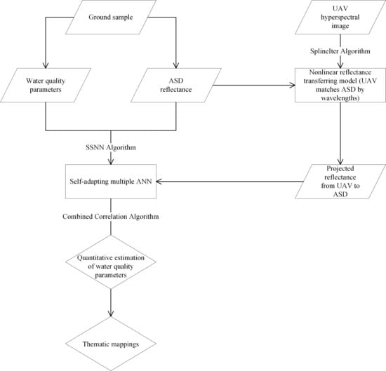
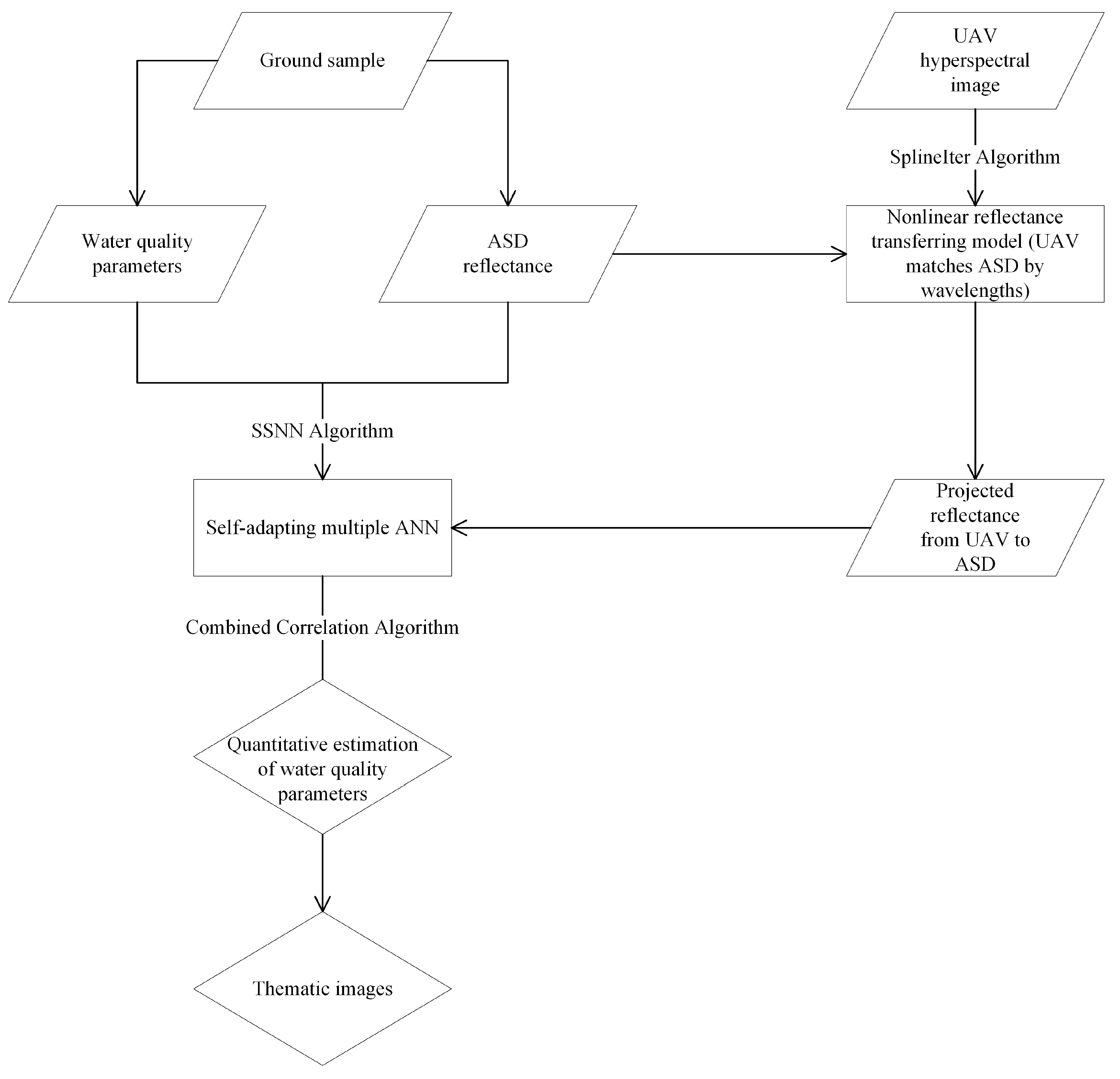
Figure 2 shows the method used to estimate the water quality parameters. First, the ground sample contains two parts, namely, ASD reflectance data and water quality parameters, which are used to establish the SSNN model. Second, the UAV hyperspectral image data in the nonlinear reflectance transferring model [49,51] are used as input to refine the data by transferring reflectance from UAV to ASD over water surface measured by ASD. Third, the transferred reflectance from UAV is used in the established SSNN model for quantitative estimation of water quality parameters, and the package of ArcGIS is used to generate thematic images.
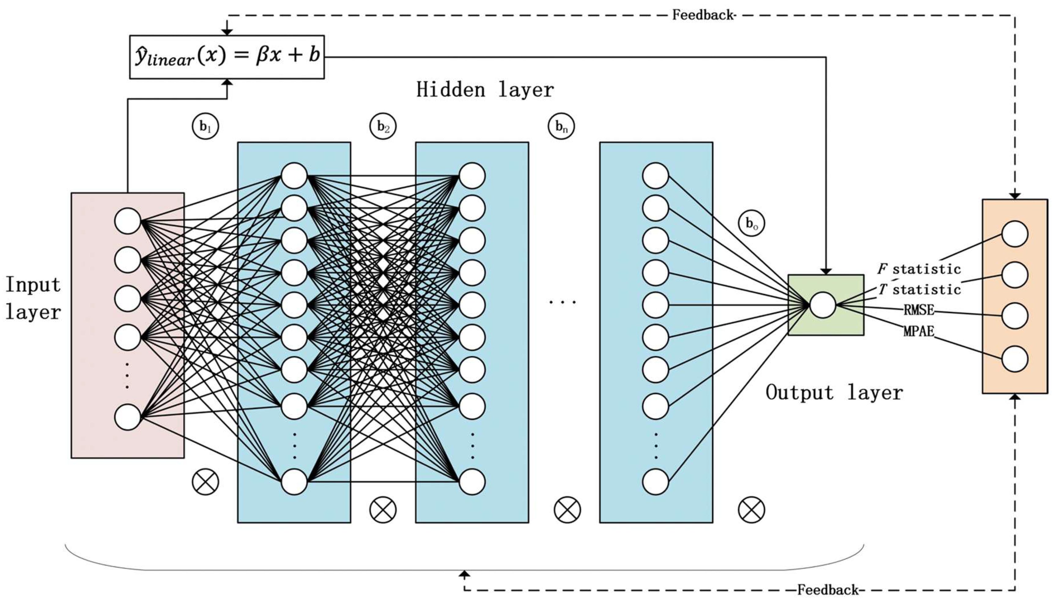
The proposed SSNN model mainly consists of three parts, namely, ANN, linear regression, and feedback machine. ANN is based on traditional ANNs of numerical prediction, including feature selection of bands, stepwise backtracking, and weight correlation. Linear regression is designed for tuning the final results. A feedback machine is dedicated for the self-adaption of the SSNN model, updating the settings for the ANN structure, such as the number of hidden layers, activation function, and the number of neurons of each hidden layer. The proposed method to monitor water quality related to ANN conducts numerical prediction on water quality parameters. Some other methods, such as combined correlation weights and the feedback machine, are incorporated into traditional ANN to quantitatively improve prediction accuracy based on a previous study [2,13,18,53,54].
The training data of SSNN includes water surface reflectance and content level of all contaminants in each point. Common ANNs with backpropagation only use one setting for all data types and ignore the changes in water bodies, resulting in low precision and compatibility. The proposed method compares all ANN-BPs to select the best one. Backpropagation, stepwise backtracking, Pearson correlation, and cosine correlation are conducted in the SSNN model. In machine learning, stepwise backtracking mathematically and computationally explains that the currently used learning rate is halved to retrain the data when the current error between the training and predicted values at current iteration step is larger than the previous error between the training and predicted values at previous iteration step. Otherwise, the halved learning rate will be halved again for small error or maintained as the current learning rate when the condition occurs again [55]. The current error between the training and predicted values is smaller than the previous error between the training and predicted values when the learning rate is small. However, the convergence rate will be slow when the initial learning rate is excessively small because no apparent changes occur between the current and previous steps, making it suitable to uses stepwise backtracking in this study. Figure 3 shows the basic structure of the improved SSNN model from traditional ANN for predicting water quality parameters. The ANN obtains the results using Equations (4)–(6). The loss function is defined as Equation (7), and the final results in the SSNN model is obtained using Equation (8),
x 1 = σ 1 ( w 1 x   + b 1 )
x 2 = σ 2 ( w 2 x 1 + b 2 )
x n = σ 2 ( w n x n 1 + b n )
= i = 1 n   ( y i y ^ i ) 2 + λ | | Θ | | | | S | |
y ^ = σ ( w l i n e a r T x + w A N N T x + b )
where x   is the input feature vector, w n is the n th step weight vector, y is the ground-measured value vector, y ^ is the predicted value vector, x n is the n th layer obtained vector, Θ denotes the set of parameters, and S denotes the set of data samples.
Various NNs with different numbers of hidden layers, numbers of nodes in each hidden layer, optimizers, and activation functions are used to choose the best NN among them on the basis of root-mean-square error (RMSE), F statistic, t statistic, and R squared value. F statistic is used to compare the statistical models fitted to the dataset to ensure the fitness of the chosen model in terms of population [56], which can be defined as Equation (9):
g F s t a t i s t i c   ( y ^ , y ) = ( T S S y ^ ,   y R S S y ^ ,   y ) / p R S S y ^ ,   y / ( n p 1 )
where T S S y ^ ,   y is the total sum of squares of y ^ and y , R S S y ^ ,   y is the residual sum of y ^ and y squares, n is the number of samples, and p is the number of features.
The F statistic plays an important and indispensable role in ANOVA. F test is defined where the null hypothesis in model 2 does not significantly fit the data better than model 1. The t statistic is used to estimate the population mean from a distribution of sample where the population standard deviation is unknown [57]. In this research, the proposed method uses the t statistic with the corresponding p-value to measure the deviation degree of the predicted values from the measured values through the mean of each group accompanied with p-value threshold set to 0.05 for rejecting the null hypothesis, where the null hypothesis is defined as the mean of predicted values is equal to the mean of measured values at 95% confidence level. The difference between two independent samples is tested, where the first one is the sample of predicted values, and the other one is the sample of measured values at 5% significance level. The formula to calculate the t statistic of two independent samples with unequal variance is obtained from Welch’s t test, as shown in Equations (10) and (11):
g W e l c h s   t t e s t   ( y ^ , y ) = y ^ m e a n y m e a n s y ^ 2 n y ^ + s y 2 n y
d f W e l c h s   t t e s t = ( s y ^ 2 n y ^ + s y 2 n y ) 2 s y ^   4 n y ^ 2 ( n y ^ 1 ) + s y   4 n y 2 ( n y 1 )
where g W e l c h s   t t e s t   ( y ^ , y ) is the t score for y ^ and y ,   d f W e l c h s   t t e s t is the degree of freedom, s is standard deviation, and n is the number of samples. The null hypothesis is that the mean of the predicting model is equal to that of the idealized model, which is distributed as the real values with respect to one of the previously mentioned water quality parameters.
The fitting model appropriately fits the data when the R 2 value is more than 0.5, otherwise it is inappropriate. The proposed method can choose a better prediction model based on the above-mentioned criteria. However, the model adopts Pearson correlation and cosine correlation to pull the predicted value deviating far from the normal volume range of the water quality parameter when the predicted value deviates from the normal range of content level of contaminants by balancing each correlation method bias and considering the weight allocation of each correlation. The working mechanism utilized in this research can be explained by the SSNN algorithm (details can be found in Algorithm A2 in the Appendix A).

4. Experimental Results

In this study, the content levels of phosphorus, nitrogen, COD, BOD, turbidity, and Chla range from 0.09 mg/L to 0.52 mg/L, from 0.09 mg/L to 5.37 mg/L, from 5.0 mg/L to 58.0 mg/L, from 1.0 mg/L to 13.9 mg/L, from 10 NTU to 97 NTU, and from 3 μ g/L to 238 μ g/L, respectively. The turbidity, Chla, BOD, COD, and nitrogen of 
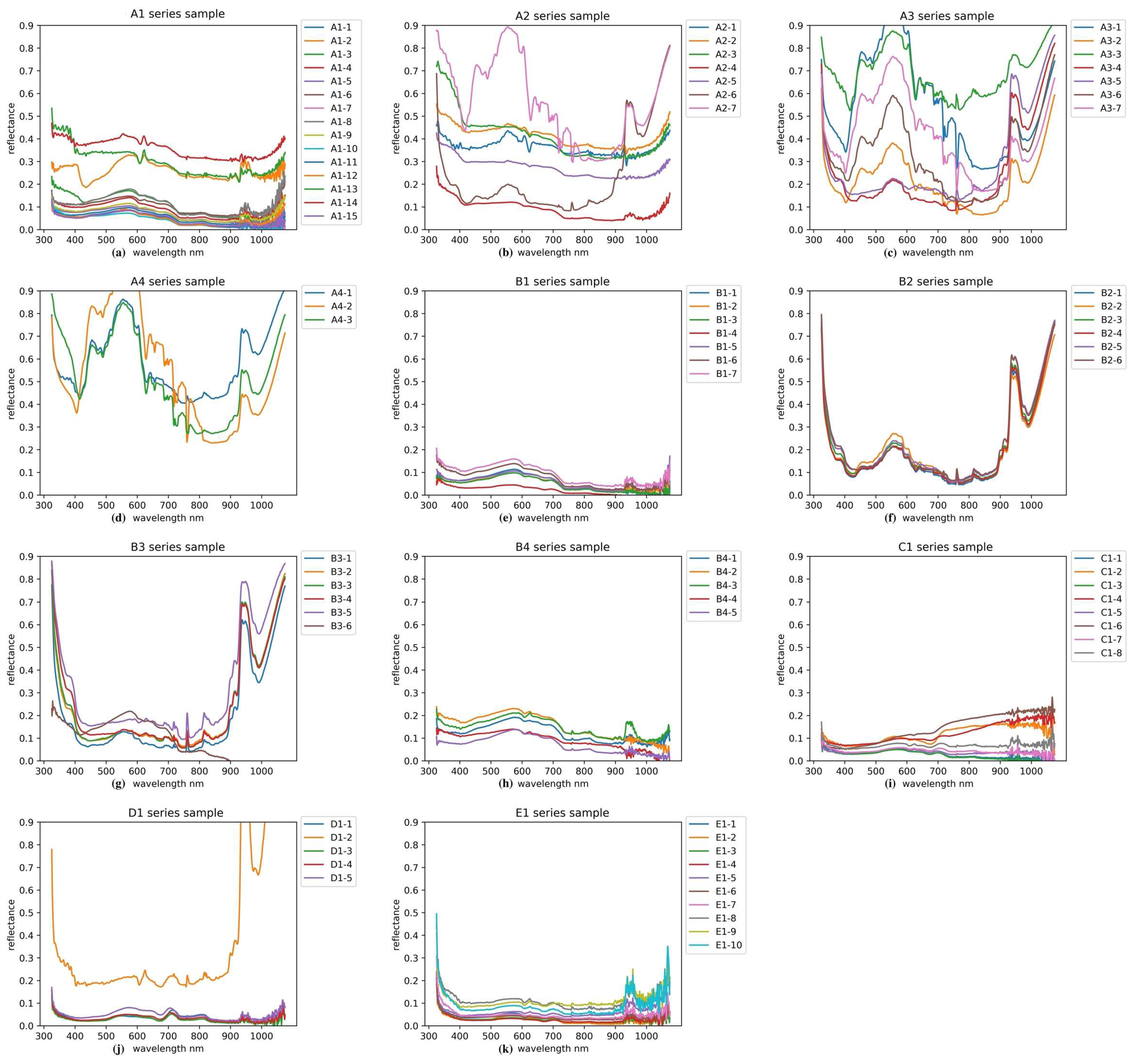
Figure 4j are the highest among the plots because the water samples are collected in fish-cultivating pools. Organic matter causes the high concentrations of BOD, COD, and nitrogen. Turbidity is highly concentrated in pools because of the absence of good outlet and inlet for water exchange, causing turbidity to rapidly increase in pools. The concentration of water quality parameters in other routes is relatively low because of the existence of water exchange and few living wastes (additional details of the sampling and measurement of water quality parameters can be found in Table 1).
Water samples were collected using a boat with ASD, and a water quality parameter instrument obtained some samples on the river concurrent with UAV taking hyperspectral images of the study area. Table 1 shows the mean and range of each parameter in the sample dataset.
Figure 4a shows the drop around 400 nm and frequent fluctuations where turbidity, BOD, and COD have relatively lower values. In Figure 4b, most points have higher reflectance compared with that of Figure 4a, and turbidity and BOD values are higher than Figure 4a. In Figure 4c, a striking jump is observed near 400 nm compared with Figure 4a, where the turbidity values are similar to that in Figure 4b but higher than that in Figure 4a. A high jump in reflectance from 900 nm to 950 nm is observed, and BOD values are lower than without an apparent reflectance jump. In Figure 4d, a situation similar to Figure 4b occurs where high BOD and turbidity values are tested. Compared with Figure 4c,d has similar trend as that in Figure 4c in which the turbidity values are relatively higher than that in Figure 4a. In Figure 4g, a small jump is observed near 800 nm, thereby explaining the higher nitrogen level higher than the previous. In Figure 4j, most reflectance has low values, a small jump is observed around 700 and 800 nm, with frequent fluctuations, but most of the corresponding parameters have the highest values among all plots. High volumes of BOD and COD match Figure 4j with a jump 700 and 950 nm and their low volumes correspond to Figure 4a going down from 600 nm to 900 nm. High Chla concentration corresponds with Figure 4j fluctuating quickly after 950 nm, and its low concentration corresponds to Figure 4f fluctuating quickly between 600 and 900 nm. For some sample reflectance plots, the bands near 400 and 900 nm may have relationships with the variation of turbidity, COD, and BOD.
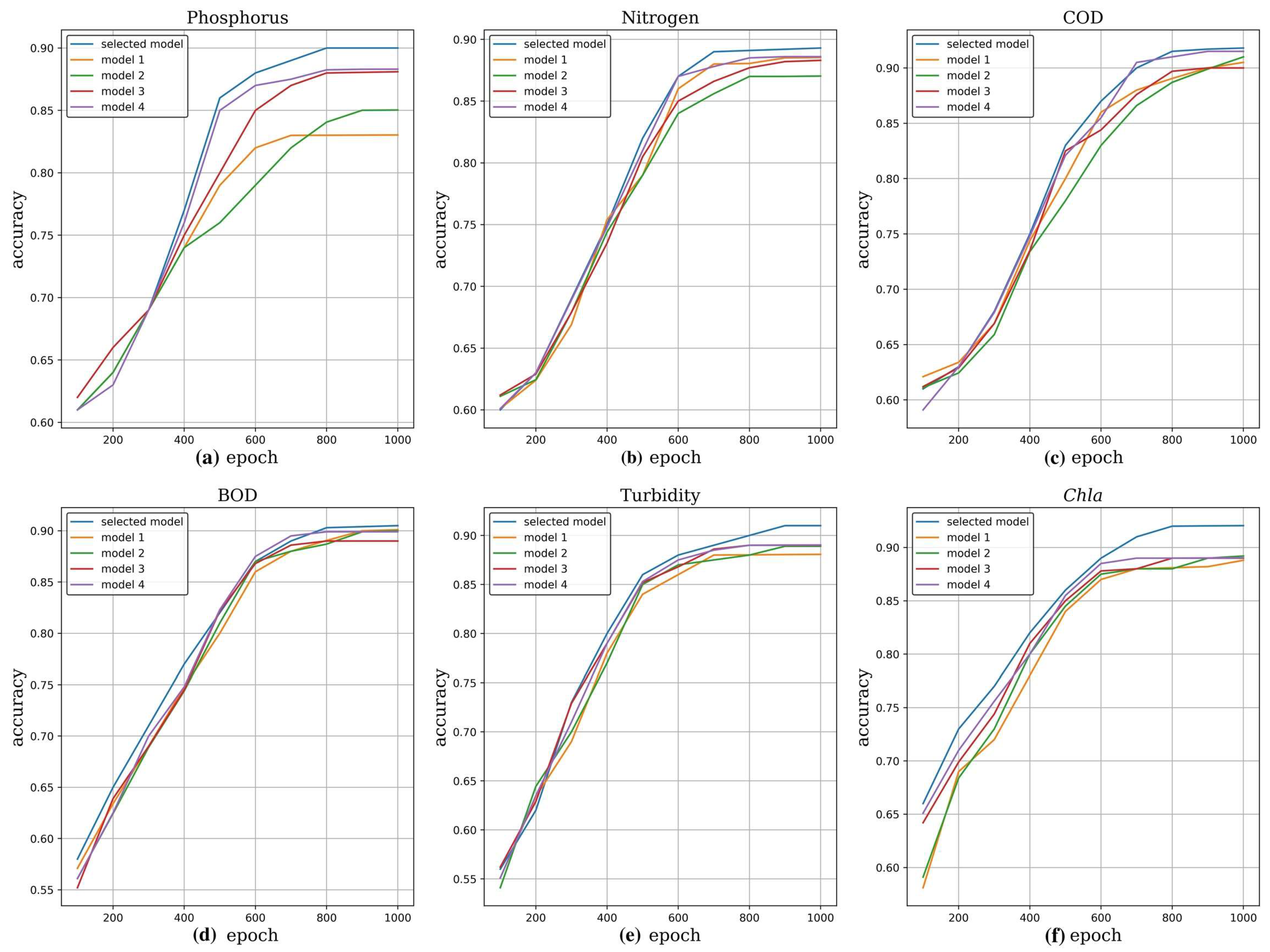
Figure 5 shows the changes in accuracy, which is defined as 1-MPAE, with the number of iterations ranging from 100 training iterations to 1000 training iterations with a step of 100 iterations and how the selected ANN-BP model outperforms the four other four models. The selected model is different from four other models in the number of hidden layers, number of hidden layer nodes, choice of optimizers, and choice of activations functions. Models 1 to 4 and the selected model are different from each other in one graph, and may not be the same as those in another graph because these models are the best models with respect to RMSE, F statistic, t statistic, and R 2 value. Models 1 to 4 in Figure 5a may be different from those in Figure 5b. If no model with respect to all criteria is constantly superior or outperforms other models in terms of RMSE, F statistic, t statistic, and R 2 value, this special case can be considered in terms of RMSE, followed by R 2 value, F statistic, and t statistic. Considering all criteria helps reduce the computational load and time of selecting the best ANN-BP model. As shown from Figure 5a–c, the selected ANN-BP model does not outperform the four other ANN-BP models under 100 iterations to 400 iterations, but gradually performs better than others. After 600 iterations, Figure 5a–c approximately obtain the relatively stable accuracy without apparent increase or decrease, and attain the balanced condition.
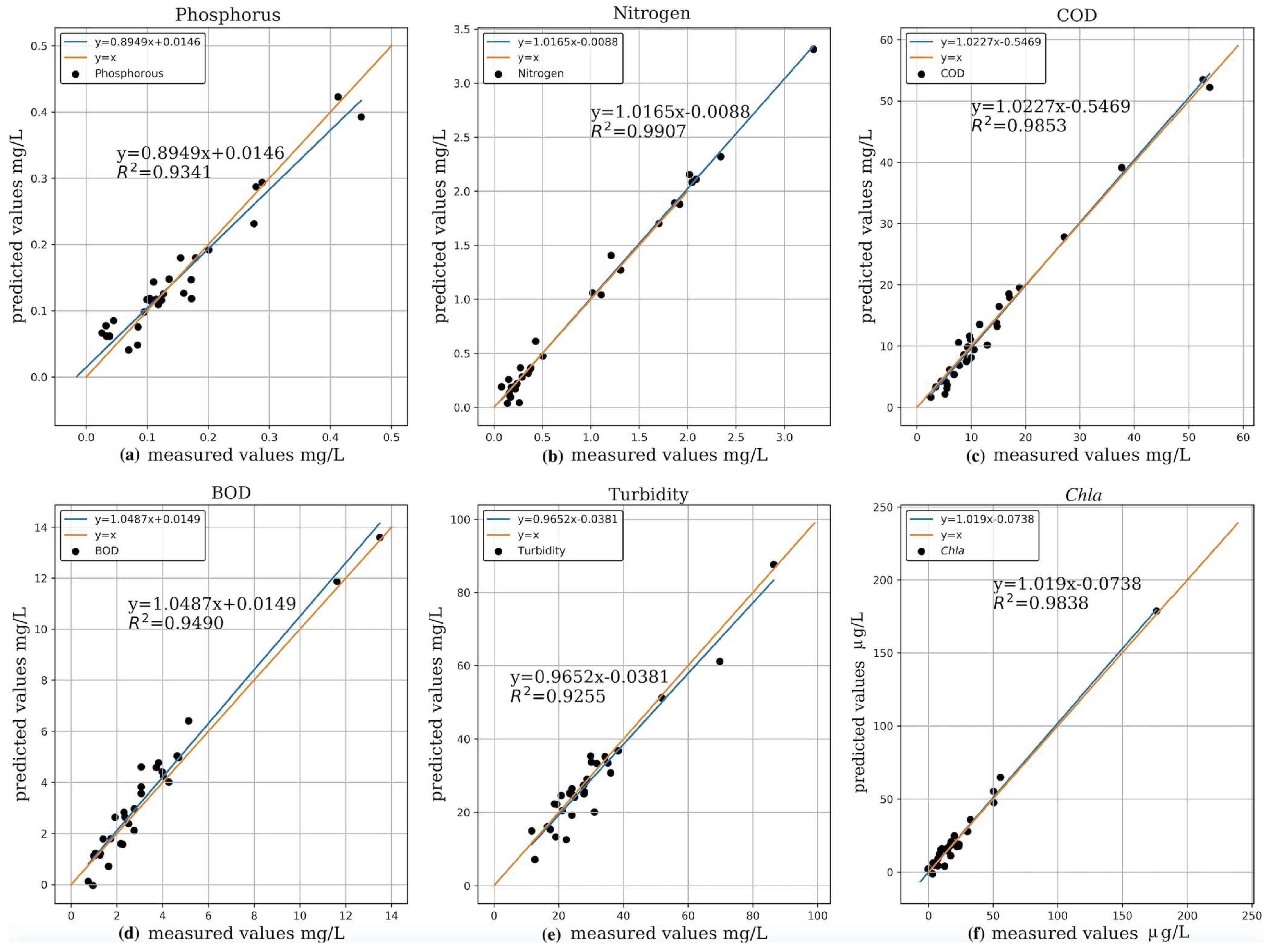
Figure 6 shows that the selected ANN-BP model fits the data better when the data are close to the orange line, explaining that the predicted values approximately match the measured values pretty using the selected ANN-BP model by the proposed SSNN. The linear relationship is established between the predicted and measured values, where the R 2 value is high in each plot, indicating the strong relationship between the predicted and measured values through a linear equation. Compared with the previously mentioned R 2 , the R 2 values in each plot of Figure 6 are given by the linear model in the same plot, and they are based on the prediction with respect to measured values rather than on the prediction with respect to reflectance. The trend can be observed by the blue line in each plot.
Table 2 gives the evaluation criteria of choosing the selected ANN-BP model and the p-value corresponding to t statistic. As shown in Table 2, turbidity and Chla generate the largest RMSE because the turbidity and Chla values are greater than others in magnitude and range of turbidity measured with unit NTU. The smallest RMSE is observed from the analysis of phosphorus because its range of values is smaller than others in magnitude. The F test with null hypothesis shows that model 2 does not significantly fit the data better than model 1. As shown in Table 2, a good ANN-BP model usually gives a large F statistic, and all models are compared with each other for only one water quality parameter. The t statistic is specified as Welch’s t test for two independent samples assuming unequal variances where the null hypothesis is that the mean of the predicting model is equal to that of the real model, which is distributed as the real values with respect to one of the water quality parameters. The confidence level is assumed to be 95%, and the significant level is 0.05. The null hypothesis is rejected when the p-value is smaller than 0.05, indicating the result is statistically significant. The p-values in Table 2 are all greater than 0.05, showing that the mean generated by one model is equal to that of the real model distributed as real values with respect to one of water quality parameters by accepting null hypothesis at 95% confidence level.
The R 2 values are all greater than 0.5, explaining that more than 50% of corresponding variance in the dependent variable can be predicted from the independent variable. In other words, more than 50% variance can be explained. The closer the R 2 value to 1 is, the better fit to data model will be.
The comparison between hyperspectral sensor to detection-needed water quality parameters and hyperspectral sensor closer to detection-needed water quality parameters help to understand the necessity of reducing the interference of such medium, such as cloud, and dust, although its corresponding R 2 values are fine. The hyperspectral images in other studies were obtained from a long distance satellite with a highly expensive and lengthy process of image retrieval that involves many interferences, such as reflection, refraction, and heterogeneous medium.
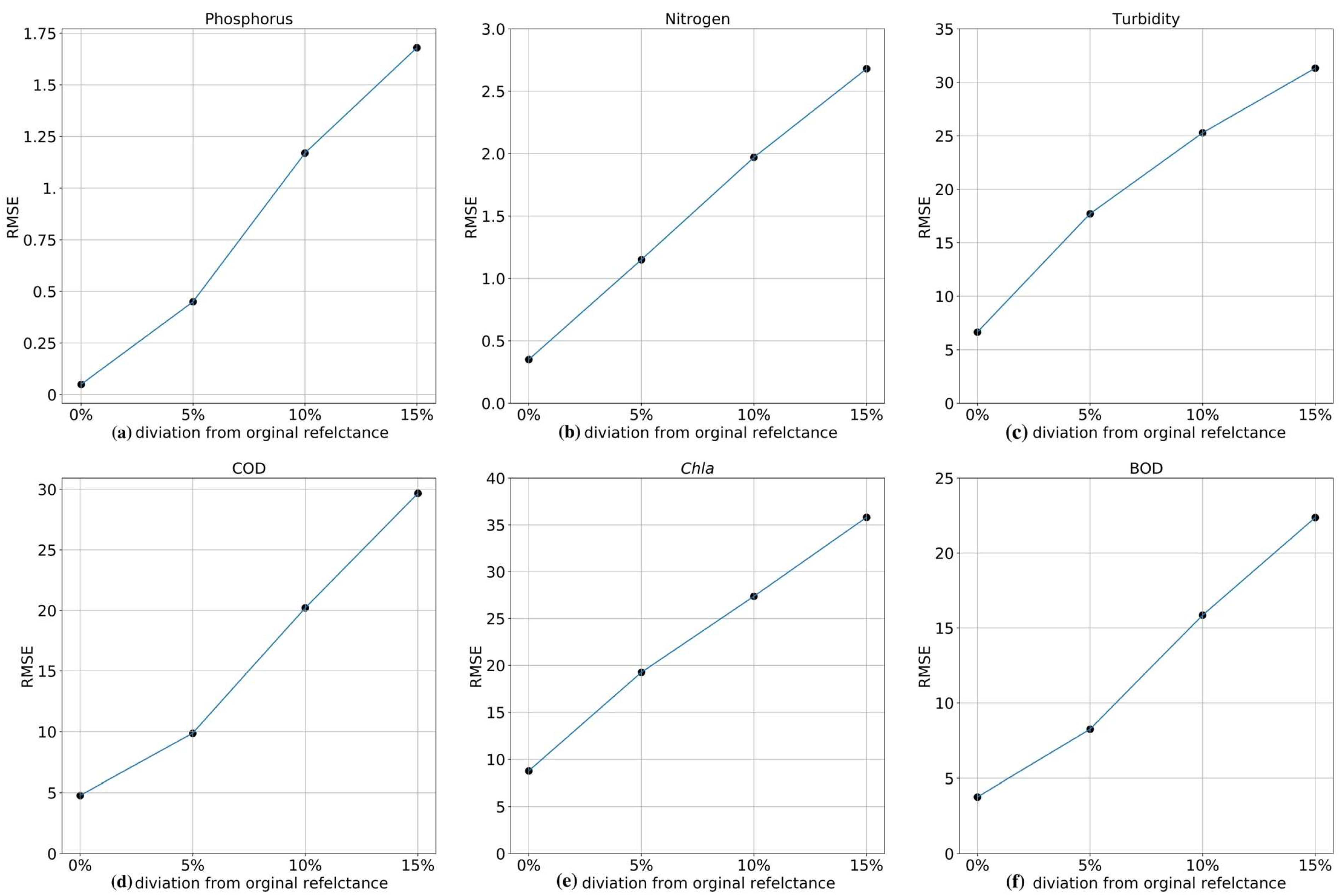
In this study, the relationship between featuring bands’ reflectance and content level of each water quality parameter is evaluated. Each graph in Figure 7 shows that the prediction with 5% deviation from bands’ reflectance performs best and provides the least RMSE compared with the two other deviated reflectance, namely, 10% and 15% deviations. Prediction with 15% deviation from bands’ reflectance gives the largest error relative to the measured values. Figure 7 shows the apparent and strong relationship between featuring bands’ reflectance and content level of each water quality parameter because of the many biases deviating from reflectance bands and the low accuracy or high RMSE for predicting the content level of water quality parameters. The water quality parameters are derived using the SSNN method with the changes in reflectance.
This research uses 30 samples as the testing dataset collected after training the data. Figure 8 shows the comparison of the predicted and ground-measured values. The proposed method accurately and quantitatively predicts nitrogen, COD, and Chla, indicating its generality and validity to predict water quality parameters.
Table 3 elucidates the performance of different methods, including SSNN, traditional single-layered ANN from Mohamad, and an empirical method from Liew et al., on the testing dataset of the entire area. The proposed method outperforms other methods in terms of RMSE and MPAE. As shown in Table 3, nitrogen calculated by SSNN achieves the best result because its MPAE is the lowest. MPAE is considered more rather than RMSE because it convincingly and effectively demonstrates the numerical prediction of the proposed method. More data should be collected from the entire area to ensure accurate numerical prediction of each water quality parameter. Therefore, more data will be collected to effectively investigate water quality in future studies. As shown in Figure 8, the R 2 value of nitrogen is larger than that of others, whereas some water quality parameters with high R 2 values may not have low MPAE because the random sample size is small, making it difficult to verify the direction of all water quality parameters. The prediction using the proposed method works properly for most of the water quality parameters, although the sample does not cover every point on the entire area where pixel points are initially spaced 40 cm apart.
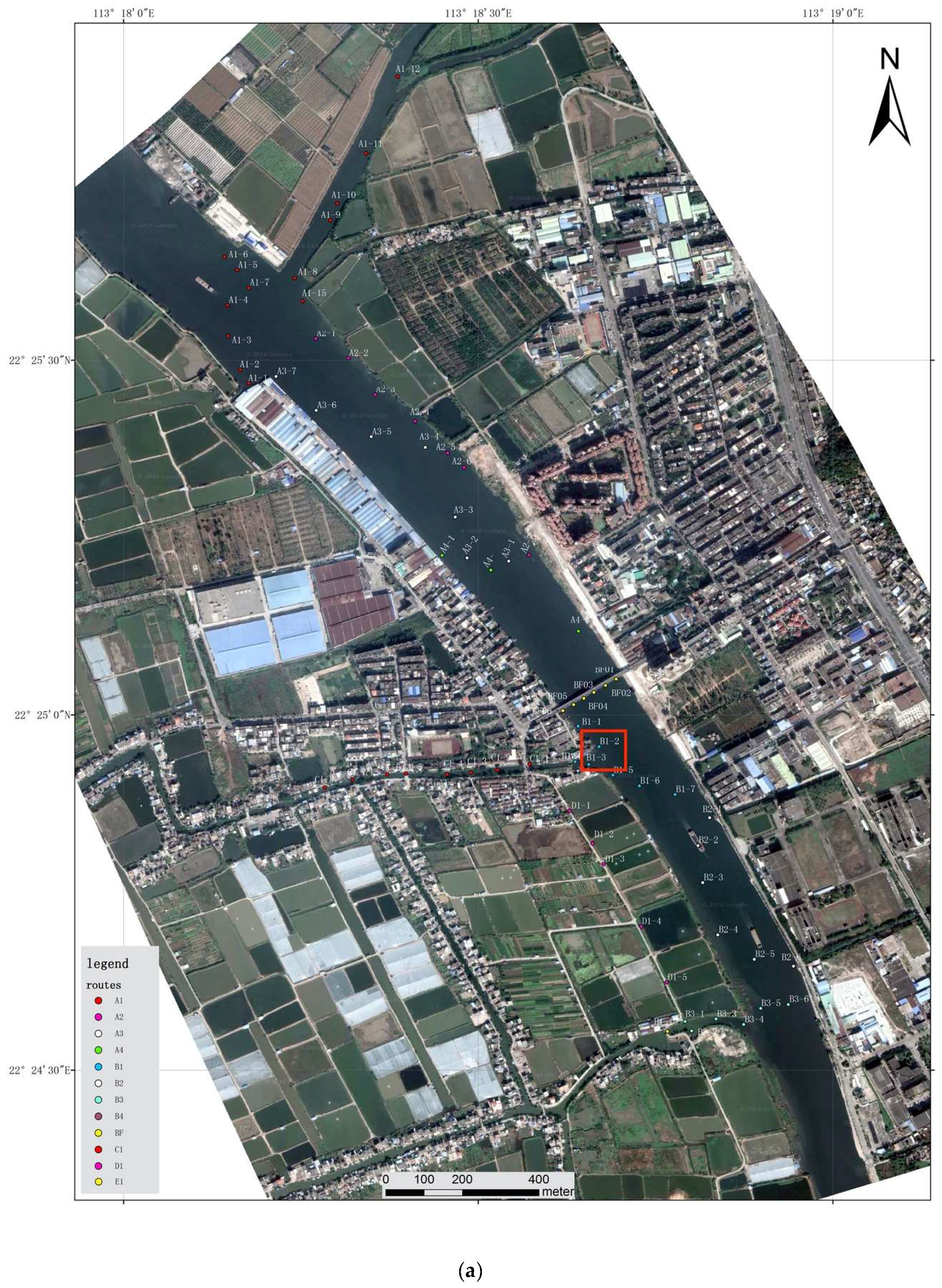
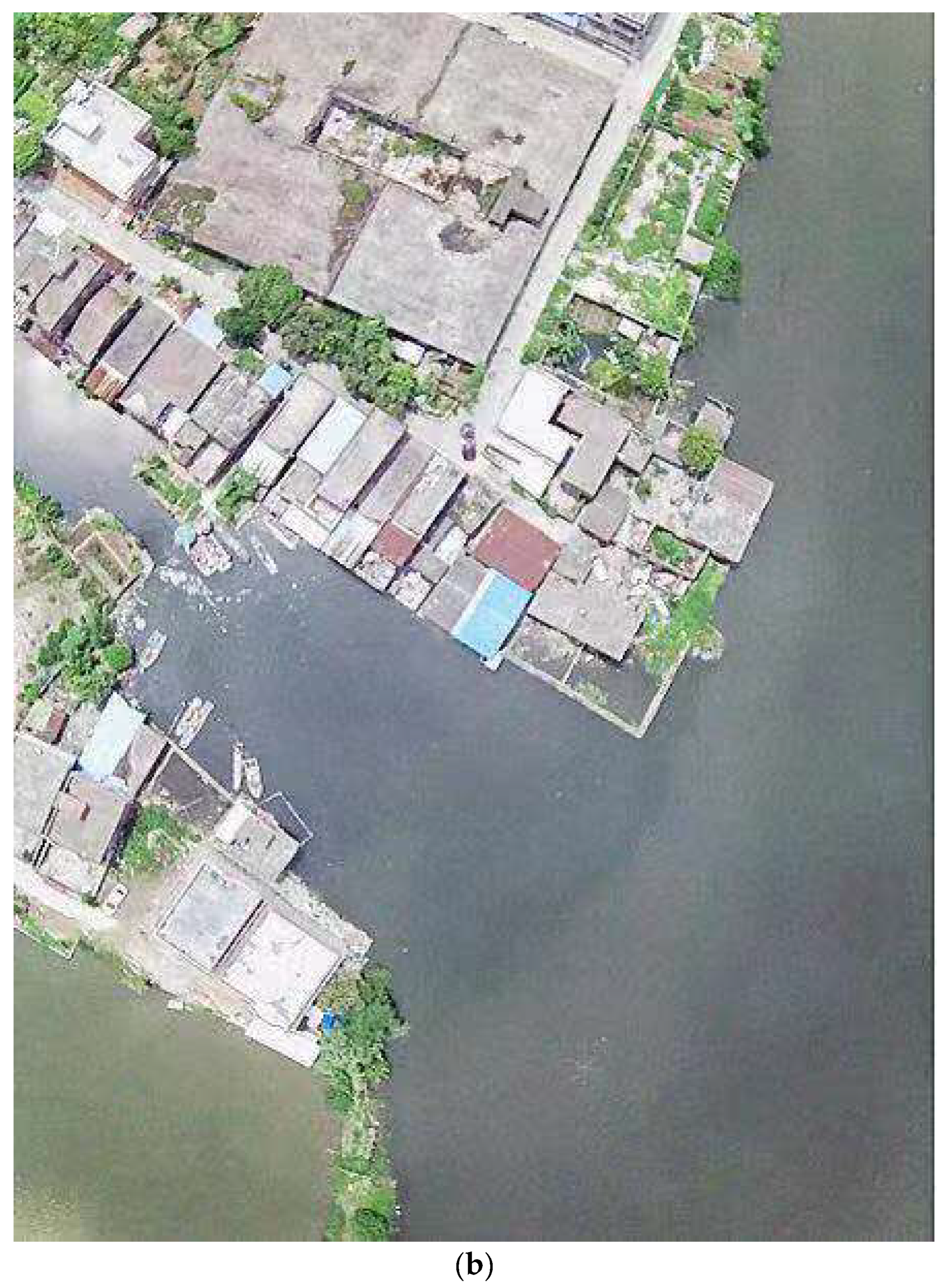
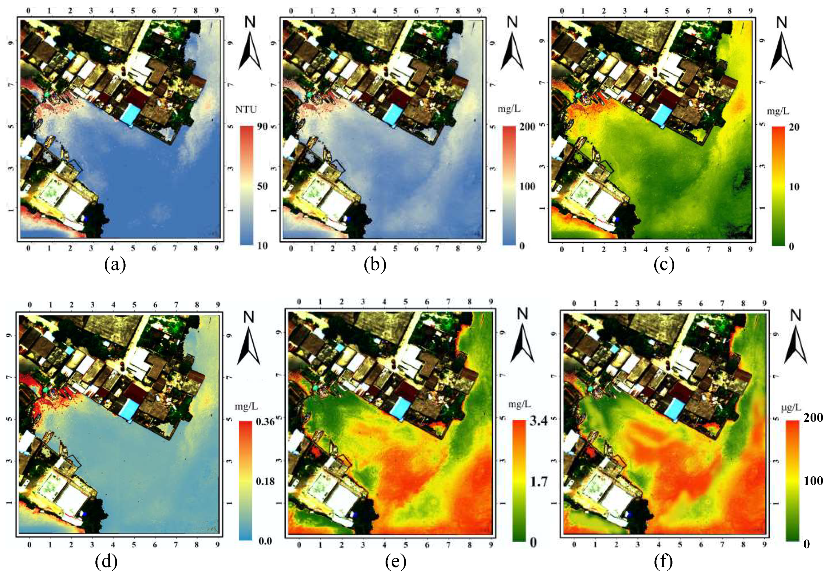
As previously mentioned, the ground ASD reflectance and water quality parameters were used as inputs to the SSNN model to establish the training model, and the UAV hyperspectral reflectance image was used as input to the SSNN model to predict the water quality parameters. Taking the small gouge marked by rectangle in the UAV image shown in Figure 1 as an example, Figure 9 shows the resulting image of the estimated water quality parameters under three wavelengths of 480, 550, and 670 nm for RGB color. In Figure 9, the distribution of each water quality parameter can be easily observed and local environment protection department can trace the distribution and the change of the content level of each water quality parameter over time to determine the source of pollution.
Although Figure 9 shows only a part of the entire study area, which is the area surrounded by red rectangle in Figure 1, its result is representative. The results show the places where people live or any factory producing leather and plastic are mostly contaminated with high contents of turbidity, COD, BOD, and phosphorus. The featuring wavelengths can quantitatively and qualitatively explain the changes in the water quality parameters. Figure 4b–d are rich in Chla, intensively fluctuating at the range of 450 and 700 nm, and Figure 4c,h have relatively high reflectance at the range of 400 nm to 900 nm corresponding to the change of above-mentioned water quality parameters over the featuring bands.

5. Discussion

In this study, we use the MPAE, RMSE, and R 2 as the criteria to determine if the proposed model fits our data properly. However, some other methods have a relatively high R 2 of 0.94 [35,54,58], and they are based on the prediction and measured values. Multiple stepwise regression analysis by Yu et al. shows the best R 2 result as 0.98 and worst R 2 result as 0.60, and that results fluctuate considerably and unstably, illustrating that the proposed method is insufficient to explain different situations or cases [34]. Some empirical methods have used dominant wavelengths that obtain poor accuracy, where the R 2 value is less than 0.7 on average [10,11,27]. Compared with some hyperbolic equations in describing the biological processes in wetlands, the traditional prediction method for the numerical values of COD is produced through linear regression [13,17]. Phuong et al. predicted BOD and COD removals through a traditional ANN method, using either COD or BOD as input in ANN to predict the other one [25], which was cost-inefficient and time-consuming. Furthermore, Mohamad’s method provided R 2 values of 0.9, but the range of measured values is too narrow to have strong representativeness such that the variation of measured values can be hardly seen [18]. He input 24 bands to his ANN model to get one output correlated with input, and the fitting process created a new mathematical function to predict the content level of Chla with only one input, the ratio of bands 671 nm and 681 nm. However, this process lost much information about other bands since only the ratio of bands 671 nm and 681 nm was considered without extracting the featuring information from other bands of initial input, 24 bands, such as that 660 nm and 665 nm are sensitive to change of the content level of Chla [30]. No concurrent sampling of remote sensing images and samples collected in the study area were conducted, resulting in an adverse effect that hyperspectral reflectance frequently changes and does not match with Chla sampling, causing the highly biased correlation relationship of his ANN-BP model and highly biased final mathematical function of predicting Chla.
The ANN method [54] by Alizadeh and Kavianpour was not generalized for other water quality parameters because some meaningful bands are neglected, and the simplified empirical equations lack scientific theoretical evidence to support themselves. The remote sensing in his study is highly expensive with a lengthy process of image retrieval and many interferences, such as reflection, refraction, and heterogeneous medium. The proposed method in this research overcomes the expensive retrieval of hyperspectral images from satellites and highly biased reflectance through concurrently cooperating work of UAV sampling and ground sampling and solves the loss of some significant information about other featuring bands using a generalized ANN-BP model for prediction rather than a highly simplified mathematical function for final prediction. Firrao et al. proposed a method [31] with accuracy achieving 75 out of 105 correctly assigned frames, illustrating that 75 of 105 testing observations are correctly classified into one of the three categories that are defined on the basis of some certain values of parameters. However, they did not consider the bands less than 750 nm that might contain some useful and important information. Their method achieved poor accuracy for the content level of fumonisins because it only classified the three class levels with R 2 value of 0.6 and prediction accuracy less than 0.8. The proposed method in this study provides a precise quantitative prediction for the water quality parameters of each pixel. In addition, the proposed method realizes the prediction for some water quality parameters and automates prediction and analysis by providing low errors and high R 2 values. For some of the above-mentioned water quality parameters, a previous study on Chla introduced a hybrid inversion method incorporating support vector machine, random forest regression [59], and other machine learning methods to predict Chla [6,60]. However, the hybrid inversion method did not consider all information in hyperspectral remote sensing images because some wavelengths with apparently different reflectance might need to be combined rather than only using one of them. Regional multiple stepwise regression ignores a large amount of features, adversely affecting the final prediction because of the importance of collinearity between bands, and its total amount of variables is approximately 20 and combined as spectral indices of reflectance, where the removal of useful and significant combinations of variables is time consuming, sophisticated, and can only predict one water quality parameter [34].
Ryan and Ali proposed a method using partial least square regression to predict each water quality-related variable [29]. However, their method could not update each parameter in partial least square regression to improve the prediction accuracy with the increase in the number of iterations, and the R 2 value (0.85) is derived from the equation established based on the relationship between the measured and predicted values, where a strong relationship is found, and a high MPAE of approximately 30% is obtained. A physics-based method using backscattering and coefficient absorption of water can be used to predict nitrogen and BOD related to water reflectance, and the optical properties could be obtained solely from the sensor data without needing additional in-situ data, where the R 2 value exceeds 0.8 through linear regression. Liew et al. proposed a method [61] that required many tests on experimental samples and empirical experiments on combinations of different bands because of the large amount of data, which is time consuming and expensive.
In Figure 9, a reasonable inference can be made that (a) has a high level near the bank where many dwellers pour their living waste, such as detergent, papers and cooking oil into the river, causing quick accumulative concentration of turbidity [24], where some of them suspend in the water surface rather than depositing at the bottom of the water, and others may deposit at the bottom of the water, causing the water to be muddy and turbid, black in color, and nontransparent. Some leather-processing and textile factories are located near the bank, and some of them discharge their industrial wastewater containing heavy metals, such as copper and lead, and dyestuff, such as bioresistant organic pollutants, as recalcitrant xenobiotic compounds that are difficult to be degraded and not exhausted on leather materials. Acid and direct trisazo dyes are dumped into the water through underwater pipes. A small accumulation of turbidity is observed in the bank because the living wastes or effluents in the industries need time and kinetic energy to transport off bank to the center of the river. Some chemical compounds consisting of heavy metals causing the water to be black and turbid cannot go far from the bank because of their weights [62]. The same condition is observed for the high concentration of phosphorus (Figure 9d) because most living wastes, such as fertilizers and laundry detergents, contain phosphorus. As shown in Figure 9d, the concentration of phosphorus near the bank is higher than that far from the bank because laundry detergents and other phosphorus-containing things, such as soap, are frequently discharged near the bank of the living area of dwellers, causing the quick increase in phosphorus. Thus, the accumulation of phosphorus near the banks is constantly higher than that in far parts toward the center of the river, although phosphorus materials may have lower weights than other metal-related materials [63].
A previous study by the local government showed that a large quantity of algae need oxygen to grow and release oxygen, resulting in a high concentration of each water quality parameter [7,32] in Figure 9b,c, indicating that the concentration of each water quality parameter from the bank is high represented by the orange band and caused by cultivation industry near the bank, and a small concentration is observed everywhere else [64]. As shown in Figure 6b,c, COD and BOD have a similar distribution of concentration near the discharge outlet close to the bank because of the need for some cultivated aquatic plants or animals, and a low concentration of COD and BOD from the bank toward the center of the river is observed, forming a curvy band of relatively dense concentration along the convex parts of the bank [36]. COD and BOD may be caused by some aquatic animals because phosphorus has a relatively low concentration, causing the normal reproduction of aquatic animals rather than hampering their reproduction [32].
As shown in Figure 9e,f, the red color represents the high concentration of nitrogen and Chla with similar distributions because nitrogen is an important water quality parameter used to synthesize Chla, and the shortage of nitrogen will stifle the synthesis and growth of Chla because nitrogen and Chla are generated by some algae off the bank aggregating as clusters [7,65]. The remains of laundry detergent and agricultural fertilizer poured into water outlets are discharged to the river by fishermen or local dwellers who live near the pools, causing algal growth associated with the high concentration of Chla [29,33]. The concentration distribution of phosphorus is similar to the concentration distribution of nitrogen and Chla for some parts near the waste discharge outlet because the rapid accumulation of phosphorus can cause water eutrophication [6,66]. Phosphorus and nitrogen are necessary for the growth of algae, and overgrowth of algae occurs in any area with high concentrations of phosphorus and nitrogen. Some detrimental chemical materials, such as copper sulfate used in agriculture or plastic-made materials, are discharged from two convex parts of the bank, thereby destroying the growth of algae near the two convex parts of the bank [7] Chemicals, such as copper sulfate, are important and beneficial for agricultural cultivation of aquatic animals, such as fish, because it works as algaecide and pesticide to prevent some fish-related diseases for agricultural cultivation of aquatic animals under regular dosage control [67]. Thus, the concentrations of BOD and COD near the convex parts of the bank are higher than other areas, whereas the concentrations of nitrogen and of Chla are lower near the convex parts of the bank and higher than other areas.
Figure 9e,f show an opposite concentration distribution to Figure 9b,c because most oxygen demands are from aquatic animals rather than from algae, and few aquatic animals can be observed because eutrophication causes the reproduction of algae to reduce the amount of nutrients for other organisms, such as fish and planktons, indicating that algae deprive the necessary nutrients, such as oxygen and nitrogen, to other organisms. Therefore, the concentration distribution of BOD and COD is different from that of nitrogen and Chla [36]. The places far from dwellers and factories are mostly contaminated with high contents of nitrogen and Chla, in which synthesis requires nitrogen because the absence of dwellers and factories enables many opportunities to be exposed to light to grow faster than others compare with those with small chance to be exposed to light where light is important and indispensable for growing of plants [65].The results show that local environmental protection department can find the sources of contamination and monitor the change in water quality of the Shiqi River in situ using the SSNN model. BOD and COD are measured through the spectrum at wavelengths ranging from 400 nm to 800 nm, which are covered in the range of bands in our research [8,13,36]. Nitrogen is measured in the spectrum ranging from 350 nm to 2500 nm [21], phosphorus apparently changes at the spectrum ranging from 400 nm to 900 nm [23], and turbidity intensively fluctuates at the spectrum ranging from 400 nm to 850 nm. Chla is mainly affected at the spectrum ranging from 450 nm to 675 nm [29], which is mostly contained within our wavelengths ranging from 404.0 nm to 894.3 nm.
There are some limitations in this study, such as limit of data volume and the uncertainty of model of transferring UAV to ASD. For some other methods [1,67], they used hundreds of samples to build and test their models where some of their water samples are deployed in laboratory but not in situ samples. However, our water samples are in situ samples, which are time-consuming and highly expensive to be chemically analyzed. And we took the samples from 11 different routes and the collected samples were relatively representative since the sample-collecting area covered certainly meaningful parts of the whole area including a heavily polluted area, a lightly polluted area, and an unpolluted area. Additionally, our proposed model is a self-adapting selection model which is able to select the best model regardless of the diversity of data, and our model can perform better so long as the volume of data meet the basic requirement of establishment of the model. In our study, 79 samples basically satisfied the requirement of establishing model since we were constrained to certain financial support and time. Nevertheless, if we obtained more water samples, the prediction model would outperform the current model in terms of its quantitative predicting accuracy. Currently, our fitted model fits our research area, but if we obtain more different data, our proposed method will fit other area as well because of the self-adaption selection ability of our model. Deep and further study will continue with more sample data for better performance and more effective monitoring of the change of water quality.

6. Conclusions

In this study, the proposed SSNN is a general method used to predict water quality parameters, including phosphorus, nitrogen, BOD, COD, turbidity, and Chla. The proposed method is improved from the conventional ANN-BP method with a fixed and simple structure that only fits its training data. Furthermore, the proposed method combines concurrent UAV and ground sampling and uses an improved ANN-BP to predict the content level of the above-mentioned water quality parameters under modified water reflectance. The hyperspectral image data needs to be transferred to match ASD ground reflectance data at each wavelength piece-wise, since estimation for each water quality parameter based on reflectance has been proved by earlier studies in Section 2.2.3. Thus, the proposed method of SSNN can quantitatively and precisely predict the content level of each water quality parameter using the featuring testing bands’ reflectance. Compared with other studies, our proposed method is novel and it predicts the quantitative content levels of water quality parameters based on hyperspectral reflectance. Furthermore, the predicting precision of the quantitative content levels of water quality parameters based on remote sensing reflectance in other studies are lower than that in our study. The R 2   values of most auto-selected models are more than 0.9, and their MPAEs are less than 10% on the testing dataset, demonstrating that the predicting model fits the data well. The R 2   values obtained using the linear regression equation established based on the measured values rather than predicted values are higher than 0.98. Thus, the proposed SSNN method outperforms other methods in terms of universality and precision.
The SSNN algorithm incorporating other algorithms, such as SplineIter (details can be found in Algorithm A1 in the Appendix A), is a relatively general means to balance the difference between the predicted and measured values through matching the featuring bands’ reflectance with most of the training similar bands’ reflectance to control the predicted values via combined correlation (details can be found in Algorithm A3 in the Appendix A). Compared with other traditional ANN-BPs, this research proposes a method combined with the above method that can select the best model with the best settings, such as the number of hidden layers, number of neurons in each hidden layer, choice of optimizer, and activation function because different data may fit different settings well. From the comparison with other studies in the methodology and experimental results, this research aims to estimate water quality parameters from a different and novel perspective and outperforms other methods in terms of diversity, universality, compatibility, and novelty because it provides higher accuracy, interpretability, and computational efficiency. Confronted with different hyperspectral reflectance data and precision requirements, our proposed method is able to self-tune to choose the best model for given data, where the only thing that needs manual manipulation is the setting threshold for each of the mathematical and statistical criteria. The proposed method is applied to hyperspectral remote sensing images collected by UAV for monitoring the water quality of the Shiqi River, Zhongshan City, Guangdong Province, China. The results indicate the locations of pollution sources.
The estimation of water quality parameters through low-valued water reflectance is relatively difficult to achieve because the content level of water quality parameters is relatively low in the Shiqi River. Thus, water quality estimation from remote sensing hyperspectral data technically obtains weak signals. Thus, the high quality of the obtained UAV data should be ensured. The current experimental instruments may not meet the requirements. The sampling conditions should be appropriately controlled. The featuring wavelengths may not be specific, and parameter-controlled experiments should be considered. The hyperspectral data are mainly obtained from the Shiqi River, and the generalization of the proposed model should be in accordance with the more accumulation of ground data.
For the results in the entire study area, the local environmental protection department randomly collected some testing samples from the entire area rather than in the study area. Future studies will focus on monitoring water quality and inversion of parameters. A cloud station for instant prediction of the content level of water-quality-related parameters can be established. An unmanned boat can be used to take water samples and measure the content level of water quality parameters that must be tested and transmit the information of the content level of these water quality parameters as samples to the cloud station, which can instantly compute the results and send them to users quickly through Wi-Fi and Bluetooth. With regard to the direction of future research, we will try to obtain more related data to build a more generalized and deepened model structure to fit a wider variety of UAV-borne hyperspectral reflectance data, which may be applied to other water bodies.

Author Contributions

Conceptualization, Y.Z. (Yishan Zhang), L.W., H.R. and Y.L. (Yu Liu); Data curation, Y.Z. (Yishan Zhang) and H.R.; Formal analysis, Y.Z. (Yishan Zhang); Funding acquisition, L.W.; Investigation, Y.Z. (Yishan Zhang), L.W., H.R., Y.Z. (Yongqian Zheng), Y.W.L. (Yaowen Liu) and J.D.; Methodology, Y.Z. (Yishan Zhang); Project administration, L.W., H.R., Y.Z. (Yongqian Zheng) and Y.W.L. (Yaowen Liu); Resources, L.W., Y.Z. (Yongqian Zheng) and Y.W.L. (Yaowen Liu); Software, Y.Z. (Yishan Zhang); Supervision, L.W., H.R., Y.Z. (Yongqian Zheng) and Y.W.L. (Yaowen Liu); Validation, Y.Z. (Yishan Zhang); Visualization, Y.Z. (Yishan Zhang), H.R. and Y.W.L. (Yaowen Liu); Writing—original draft, Y.Z. (Yishan Zhang); Writing—review & editing, L.W., H.R. and Y.L. (Yu Liu). All authors have read and agreed to the published version of the manuscript.

Funding

This research is supported by Shenzhen Intelligent River pilot program (SZCG2018159487), National Natural Science Foundation of China (No. 41771369), and Smart Guangzhou Spatio-temporal Information Cloud Platform Construction (GZIT2016-A5-147).

Acknowledgments

The authors extend particular thanks to the Shenzhen Huahan Technology companies for providing the hyperspectral images and ground measurement data.

Conflicts of Interest

The authors declare that we have no financial and personal relationships with other people or organizations that can inappropriately influence our work and that this paper was not published before, the founding sponsors had no role in the design of the study; in the collection, analyses, or interpretation of data; in the writing of the manuscript, and in the decision to publish the results.

Appendix A

Algorithm A1. SplineIter for linear regression between the ASD and UAV reflectance
1: n c o m m o n the   number   of   common   and   concurrent   data   of   UAV   and   ASD
2: n U A V the   number   of   wavelengths   data   of   UAV  
3: ρ A S D relfectance   in   data   from   ASD
4: ρ U A V relfectance   in   data   from   UAV
5: f u n t c i o n   SplineIter   ( d a t a t r a i n )
6:    f o r   i   1   to   n u a v   d o
7:      x null   list
8:      y null   list
9:      f o r   j 1   to   n c o m m o n   d o
10:        y ρ A S D [ j ] [ i ]
11:        x ρ U A V [ j ] [ i ]
12:        r e g sec ond   order   nonlinear   regression
13:        c o e f s coefficients   and   intercept   from   r e g
14:      e n d   f o r
15:    e n d   f o r
16: r e t u r n   c o e f s
17: e n d   f u n c t i o n
Algorithm A2. SSNN for selecting the best model for predicting the substances on the basis of some statistical criteria.
1: I n p u t : a   training   dataset   d a t a t r a i n   and   a   testing   dataset   d a t a t e s t
2: O u t p u t : the   model   with   better   fit   to   data ,   m
3: P r o c e d u r e : self adapting   selecting   model
4:    n t r a i n length   of   d a t a t r a i n
5:    n t e s t length   of   d a t a t e s t
6:    x t r a i n input   of   d a t a t r a i n
7:    x t e s t input   of   d a t a t e s t
8:    y t r a i n output   of   d a t a t r a i n
9:    y t e s t length   of   d a t a t e s t
10:    o h options   of   the   number   of   hidden   layers
11:    o h n options   of   the   number   of   hidden   layer   neurons
12:    o a f options   of   the   types   of   activation   functions
13:    o a l l combination   of   o h ,   o h n ,   and   o a f
14:    n n ( x ) stepwise   backtracking   neural   network   with   a   set   of   attribute ,   x
15:    i t e r m a x maximum   number   of   training   iterations
16:    f o r   i   1   to   n t r a i n   d o
17:      d a t a t r a i n ( i )   value   interpolation   ( d a t a t r a i n ( i ) )
18:      d a t a t r a i n ( i )   S p l i n e I t e r   ( d a t a t r a i n ( i ) )
19:    e n d   f o r
20:    f o r   i   1   to   n t e s t   d o
21:      d a t a t e s t ( i )   value   interpolation   ( d a t a t e s t ( i ) )
22:      d a t a t e s t ( i )   S p l i n e I t e r   ( d a t a t e s t ( i ) )
23:   e n d   f o r
24:    initialize   all   parameters   as   mentioned   before
25:    f o r   i   i n   o a l l   d o
26:      f o r   j   1   to   n t r a i n   d o
27:        f o r   k 1   to   i t e r m a x   d o
28:          n n n n ( { i , j } )
29:          update   parameters   from   n n
30:        e n d   f o r
31:      e n d   f o r
32:    e n d   f o r
33:    add   results   from   nonlinear   regression   and   n n
34:    update   parameters
35:    f o r   i   i n   o a l l   d o
36:      f o r   j   1   to   n t e s t   d o
37:        p W e l c h s   t   t e s t   calculate   corresponding   p v a l u e
38:        f   F   t e s t   to   F   statistic
39:        R 2 coefficient   of   determination
40:        ϵ error   calculated   from   n n ( { i , j } )
41:        c r t . add (   object ( n n ( { i , j } ) ) ,   ϵ , p ,   f ,   R 2 )
42:      e n d   f o r
43:    e n d   f o r
44:    c r t . sort ( k e y = o b j e c t . g e t ( ϵ ,   p ,   f ,   R 2
45:    Feedback   machine   gives   feedback   to   model   m
46: e n d   P r o c e d u r e
Algorithm A3. Final predicted outputs by correcting some anomalous values caused by systematic errors of measuring instruments.
1: I n p u t : a   predicting   dataset   d a t a p   and   the   entire   dataset   d a t a e
2: O u t p u t : quantitative   content   level   of   each   water   quality   parameter
3: f u n c t i o n : Combined   Correlation
4:    r o w s the   number   of   rows   of   d a t a p
5:    c o l s the   number   of   columns   of   d a t a p
6:    n e the   number   of   observations   of   d a t a e
7:    x e the   reflectance   corresponding   to   certain   wavelengths   in   d a t a e
8:    y e quantitative   content   level   of   each   water   quality   parameter   in   d a t a e
9:    x p the   reflectance   corresponding   to   certain   wavelengths   in   d a t a p
10:    y p quantitative   content   level   of   each   water   quality   parameter   in   d a t a p
11:    n n the   selected   stepwise   backtracking   neural   network
12:    f o r   i   1   to   n e   d o
13:      d a t a e ( i )   value   interpolation   ( d a t a e ( i ) )
14:      d a t a e ( i )   S p l i n e I t e r   ( d a t a e ( i ) )
15:    e n d   f o r
16:    f o r   i   1   to   r o w s * c o l s   d o
17:      d a t a p ( i )   value   interpolation   ( d a t a p ( i ) )
18:      d a t a p ( i )   S p l i n e I t e r   ( d a t a p ( i ) )
19:    e n d   f o r
20:    f o r   i   1   to   r o w s   d o
21:      f o r   j   1   to   c o l s   d o
22:        y p ( i , j ) n n ( d a t a p ( i , j ) )
23:        i f   y p ( i , j ) > max ( y e )   o r   y p ( i , j ) < min ( y e )   t h e n
24:          f o r   k   1   to   n e 1   d o
25:            P e a r s o n m a x max ( P e a r s o n ( x e ( k ) , x p ( i , j ) ) ,   P e a r s o n ( x e ( k + 1 ) , x p ( i , j ) )
26:            C o s i n e m a x max ( C o s i n e ( x e ( k ) , x p ( i , j ) ) ,   C o s i n e ( x e ( k + 1 ) , x p ( i , j ) )
27:            t o t a l P e a r s o n m a x + C o s i n e m a x
28:          e n d   f o r
29:          w c P e a r s o n m a x t o t a l + C o s i n e m a x t o t a l
30:        e l s e
31:          c o n t i n u e ;
32:        e n d   i f
33:      e n d   f o r
34:    e n d   f o r
35: e n d   f u n c t i o n

References

  1. Tan, J.; Cherkauer, K.A.; Chaubey, I. Using hyperspectral data to quantify water-quality parameters in the Wabash River and its tributaries, Indiana. Int. J. Remote Sens. 2015, 36, 5466–5484. [Google Scholar] [CrossRef]
  2. Dodds, W.K.; Smith, V.H. Nitrogen, phosphorus, and eutrophication in streams. Inland Waters 2016, 6, 155–164. [Google Scholar] [CrossRef]
  3. Guo, Q.; Wu, X.; Bing, Q.; Pan, Y.; Wang, Z.; Fu, Y.; Wang, D.; Liu, J. Study on retrieval of chlorophyll-a concentration based on Landsat OLI Imagery in the Haihe River, China. Sustainability 2016, 8, 758. [Google Scholar] [CrossRef] [Green Version]
  4. Xiong, J.; Lin, C.; Ma, R.; Cao, Z. Remote Sensing Estimation of Lake Total Phosphorus Concentration Based on MODIS: A Case Study of Lake Hongze. Remote Sens. 2019, 11, 2068. [Google Scholar] [CrossRef] [Green Version]
  5. Skeffington, R.A.; Willson, E.J. Excess nitrogen deposition: Issues for consideration. Environ. Pollut. 1988, 54, 159–184. [Google Scholar] [CrossRef]
  6. Bennett, E.M.; Carpenter, S.R.; Caraco, N.F. Human Impact on Erodable Phosphorus and Eutrophication: A Global Perspective: Increasing accumulation of phosphorus in soil threatens rivers, lakes, and coastal oceans with eutrophication. BioScience 2001, 51, 227–234. [Google Scholar] [CrossRef]
  7. Matthews, M.W.; Bernard, S.; Winter, K. Remote sensing of cyanobacteria-dominant algal blooms and water quality parameters in Zeekoevlei, a small hypertrophic lake, using MERIS. Remote Sens. Environ. 2010, 114, 2070–2087. [Google Scholar] [CrossRef]
  8. Jouanneau, S.; Recoules, L.; Durand, M.; Boukabache, A.; Picot, V.; Primault, Y.; Lakel, A.; Sengelin, M.; Barillon, B.; Thouand, G. Methods for assessing biochemical oxygen demand (BOD): A review. Water Res. 2014, 49, 62–82. [Google Scholar] [CrossRef]
  9. Vega, M.; Pardo, R.; Barrado, E.; Deban, L. Assessment of seasonal and polluting effects on. the quality of river water by exploratory data analysis. Water Res. 1998, 32, 3581–3592. [Google Scholar] [CrossRef]
  10. Bansod, B.; Singh, R.; Thakur, R. Analysis of water quality parameters by hyperspectral. imaging in Ganges River. Spat. Inf. Res. 2018, 26, 203–211. [Google Scholar] [CrossRef]
  11. Liu, J.; Zhang, Y.; Yuan, D.; Song, X. Empirical estimation of total nitrogen and total phosphorus concentration of urban water bodies in china using high resolution ikonos multispectral imagery. Water 2015, 7, 6551–6573. [Google Scholar] [CrossRef] [Green Version]
  12. Markogianni, V.; Kalivas, D.; Petropoulos, G.; Dimitriou, E. An appraisal of the potential of Landsat 8 in estimating chlorophyll-a, ammonium concentrations and other water quality indicators. Remote Sens. 2018, 10, 1018. [Google Scholar] [CrossRef] [Green Version]
  13. Akratos, S.C.; Papaspyros, J.N.E.; Tsihrintzis, V.A. An artificial neural network model and design equations for BOD and COD removal prediction in horizontal subsurface flow constructed wetlands. Chem. Eng. J. 2008, 143, 96–110. [Google Scholar] [CrossRef]
  14. Bramante, J.; Sin, T. Optimization of a Semi-Analytical Algorithm for Multi-Temporal Water Quality Monitoring in Inland Waters with Wide Natural Variability. Remote Sens. 2015, 7, 16623–16646. [Google Scholar] [CrossRef] [Green Version]
  15. Liu, X.; Sun, Q.; Meng, Y.; Fu, M.; Bourennane, S. Hyperspectral image classification based on parameter-optimized 3D-CNNs combined with transfer learning and virtual samples. Remote Sens. 2018, 10, 1425. [Google Scholar] [CrossRef] [Green Version]
  16. Palani, S.; Liong, S.Y.; Tkalich, P. An ANN application for water quality forecasting. Marine Pollution Bulletin. 2008, 56, 1586–1597. [Google Scholar] [CrossRef] [PubMed]
  17. Amanollahi, J.; Kaboodvandpour, S.; Majidi, H. Evaluating the accuracy of ANN and LR models to estimate the water quality in Zarivar International Wetland, Iran. Nat. Hazards 2017, 85, 1511–1527. [Google Scholar] [CrossRef]
  18. Mohamad, A. Sea water chlorophyll-a estimation using hyperspectral images and supervised Artificial Neural Network. Ecol. Inform. 2014, 24, 60–68. [Google Scholar]
  19. Bao, Y.; Tian, Q.; Chen, M. A weighted algorithm based on normalized mutual information for estimating the chlorophyll-a concentration in inland waters using Geostationary Ocean Color Imager (GOCI) data. Remote Sens. 2015, 7, 11731–11752. [Google Scholar] [CrossRef] [Green Version]
  20. Blix, K.; Li, J.; Massicotte, P.; Matsuoka, A. Developing a New Machine-Learning Algorithm for Estimating Chlorophyll-a Concentration in Optically Complex Waters: A Case Study for High Northern Latitude Waters by Using Sentinel 3 OLCI. Remote Sens. 2019, 11, 2076. [Google Scholar] [CrossRef] [Green Version]
  21. Karimi, Y.; Prasher, S.O.; McNairn, H.; Bonnell, R.B.; Dutilleul, P.; Goel, P.K. Discriminant. Analysis of Hyperspectral Data for Assessing Water and Nitrogen Stresses in Corn. Am. Soc. Agric. Biol. Eng. 2005, 8, 805–813. [Google Scholar] [CrossRef]
  22. Hashitani, H.; Okumura, M. A simple visual method for the determination of phosphorus in environmental waters. Anal. Bioanal. Chem. 1978, 328, 251–254. [Google Scholar] [CrossRef]
  23. Song, K.; Li, L.; Li, S.; Tedesco, L.; Hall, B.; Li, L. Hyperspectral remote sensing of total phosphorus (TP) in three central Indiana water supply reservoirs. Water Air Soil Pollut. 2012, 223, 1481–1502. [Google Scholar] [CrossRef]
  24. Saluja, R.; Garg, J.K. Characterization and modeling of bio-optical properties of water in a. lentic ecosystem using in-situ hyperspectral remote sensing. In Remote Sensing of the Oceans and Inland Waters: Techniques, Applications, and Challenges; SPIE Asia-Pacific Remote Sensing: New Delhi, India, 2016; Volume 9878, p. 98780Y. [Google Scholar]
  25. Phuong, T.B.N.; Tri, V.P.D.; Duy, N.B.; Nghiem, N.C. Remote Sensing for Monitoring. Surface Water Quality in the Vietnamese Mekong Delta: The Application for Estimating Chemical Oxygen Demand in River Reaches in Binh Dai, Ben Tre. Vietnam J. Earth Sci. 2017, 39, 256–269. [Google Scholar] [CrossRef] [Green Version]
  26. Salem, S.; Higa, H.; Kim, H.; Kazuhiro, K.; Kobayashi, H.; Oki, K.; Oki, T. Multi-algorithm indices and look-up table for chlorophyll-a retrieval in highly turbid water bodies using multispectral data. Remote Sens. 2017, 9, 556. [Google Scholar] [CrossRef] [Green Version]
  27. Rostom, G.N.; Shalaby, A.A.; Issa, Y.M.; Afifi, A.A. Evaluation of Mariut Lake water. quality using Hyperspectral Remote Sensing and laboratory works. Egypt. J. Remote Sens. Space Sci. 2017, 20, 39–48. [Google Scholar] [CrossRef] [Green Version]
  28. Hansen, C.; Williams, G. Evaluating Remote Sensing Model Specification Methods for Estimating Water Quality in Optically Diverse Lakes throughout the Growing Season. Hydrology 2018, 5, 62. [Google Scholar] [CrossRef] [Green Version]
  29. Ryan, K.; Ali, K. Application of a Partial Least-Squares Regression Model to Retrieve Chlorophyll-a Concentrations in Coastal Waters using Hyper-Spectral Data. Ocean Sci. J. 2016, 51, 209–221. [Google Scholar] [CrossRef]
  30. Pyo, J.; Pachepsky, Y.; Baek, S.-S.; Kwon, Y.; Kim, M.; Lee, H.; Park, S.; Cha, Y.; Ha, R.; Nam, G. Optimizing semi-analytical algorithms for estimating chlorophyll-a and phycocyanin concentrations in inland waters in Korea. Remote Sens. 2017, 9, 542. [Google Scholar] [CrossRef] [Green Version]
  31. Firrao, G.; Torelli, E.; Gobbi, E.; Raranciuc, S.; Bianchi, G.; Locci, R. Prediction of milled. maize fumonisin contamination by multispectral image analysis. J. Cereal Sci. 2010, 52, 327–330. [Google Scholar] [CrossRef]
  32. Glibert, M.P. Eutrophication, harmful algae and biodiversity—Challenging paradigms in a world of complex nutrient changes. Mar. Pollut. Bull. 2017, 124, 591–606. [Google Scholar] [CrossRef] [PubMed]
  33. Gitelson, A. The peak near 700 nm on radiance spectra of algae and water: Relationships of its. magnitude and position with chlorophyll concentration. Int. J. Remote Sens. 1992, 13, 3367–3373. [Google Scholar] [CrossRef]
  34. Yu, X.; Yi, H.; Liu, X.; Wang, Y.; Liu, X.; Zhang, H. Remote-sensing estimation of dissolved inorganic nitrogen concentration in the Bohai Sea using band combinations derived from MODIS data. Int. J. Remote Sens. 2016, 37, 327–340. [Google Scholar] [CrossRef]
  35. Friedrichs, A.; Busch, J.A.; Woerd, H.J.V.D.; Oliver, Z. SmartFluo: A method and affordable adapter to measure chlorophyll a fluorescence with smartphones. Sensors 2017, 17, 678. [Google Scholar] [CrossRef] [PubMed] [Green Version]
  36. Lee, J.; Lee, S.; Yu, S.; Rhew, D. Relationships between water quality parameters in rivers and lakes: BOD 5, COD, NBOPs, and TOC. Environ. Monit. Assess. 2016, 188, 252. [Google Scholar] [CrossRef]
  37. Zhou, L.; Ma, W.; Zhang, H.; Li, L.; Tang, L. Developing a PCA–ANN model for predicting chlorophyll a concentration from field hyperspectral measurements in Dianshan Lake, China. Water Qual. Expo. Health 2015, 7, 591–602. [Google Scholar] [CrossRef]
  38. Wang, Z.; Kawamura, K.; Sakuno, Y.; Fan, X.; Gong, Z.; Lim, J. Retrieval of chlorophyll-a and total suspended solids using iterative stepwise elimination partial least squares (ISE-PLS) regression based on field hyperspectral measurements in irrigation ponds in Higashihiroshima, Japan. Remote Sens. 2017, 9, 264. [Google Scholar] [CrossRef] [Green Version]
  39. Yang, M.; Ishizaka, J.; Goes, J.; Gomes, H.; Maúre, E.; Hayashi, M.; Katano, T.; Fujii, N.; Saitoh, K.; Mine, T. Improved MODIS-Aqua chlorophyll-a retrievals in the turbid semi-enclosed Ariake Bay, Japan. Remote Sens. 2018, 10, 1335. [Google Scholar] [CrossRef] [Green Version]
  40. Deaconu, M.; Senin, R.; Stoica, R.; Athanasiu, A.; Crudu, M.; Oproiu, L.; Ruse, M.; Filipescu, C. Adsorption decolorization technique of textile/leather–dye containing effluents. Int. J. Waste Resour. 2016, 6, 212–218. [Google Scholar] [CrossRef] [Green Version]
  41. Zhang, G.; Zeng, G.; Cai, X.; Deng, S.; Luo, H.; Sun, G. Brachybacterium zhongshanense sp. nov., a cellulose-decomposing bacterium from sediment along the Qijiang River, Zhongshan City, China. Int. J. Syst. Evol. Microbiol. 2007, 57, 2519–2524. [Google Scholar] [CrossRef]
  42. Zhou, H.; Wong, M. Screening of Organochlorines in Freshwater Fish Collected from the Pearl. River Delta, People’s Republic of China. Arch. Environ. Contam. Toxicol. 2004, 46, 106–113. [Google Scholar] [CrossRef] [PubMed]
  43. Cai, J.; Cai, Y.; Tan, H.; Wang, Y.; Luo, J. Fractionation and ecological risk in urban river. sediments in zhongshan city, Pearl River Delta. J. Environ. Monit. 2011, 13, 2450–2456. [Google Scholar] [CrossRef] [PubMed]
  44. Scott, J.; Tuma, M. Preconditioning of Linear Least Squares by Robust Incomplete Factorization for Implicitly Held Normal Equations. SIAM J. Sci. Comput. 2016, 38, 603–623. [Google Scholar] [CrossRef] [Green Version]
  45. Ruddick, K.G.; Voss, K.; Boss, E.; Castagna, A.; Frouin, R.; Gilerson, A.; Hieronymi, M.; Johnson, B.C.; Kuusk, J.; Lee, Z.; et al. A Review of Protocols for Fiducial Reference Measurements of Downwelling Irradiance for the Validation of Satellite Remote Sensing Data over Water. Remote Sens. 2019, 11, 1742. [Google Scholar] [CrossRef] [Green Version]
  46. Zhang, S.; Du, M.; Qu, L. Modified DAT/IAT Process for Removal of Ammonia Nitrogen. from Domestic Sewage. In Proceedings of the 2nd International Conference on Bioinformatics and Biomedical Engineering (BBE, 2008), Shanghai, China, 16–18 May 2008; pp. 3295–3299. [Google Scholar]
  47. Hejzlar, J.; Kopáček, J. Determination of Low Chemical Oxygen Demand Values in Water by the Dichromate Semi-micro Method. Analyst 1990, 115, 1463–1467. [Google Scholar] [CrossRef]
  48. Gohin, F. Annual cycles of chlorophyll-a, non-algal suspended particulate matter, and turbidity. observed from space and in-situ in coastal waters. Ocean Sci. 2011, 7, 705–732. [Google Scholar] [CrossRef] [Green Version]
  49. Su, T.C. A study of a matching pixel by pixel (MPP) algorithm to establish an empirical model of water quality mapping, as based on unmanned aerial vehicle (UAV) images. Int. J. Appl. Earth Obs. Geoinf. 2017, 58, 213–224. [Google Scholar] [CrossRef]
  50. Zeng, C.; Richardson, M.; King, D.J. The impacts of environmental variables on water reflectance measured using a lightweight unmanned aerial vehicle (UAV)-based spectrometer system. ISPRS J. Photogramm. Remote Sens. 2017, 130, 217–230. [Google Scholar] [CrossRef]
  51. Guimaraes, T.T.; Veronez, M.R.; Koste, E.C.; Gonzaga, L.; Bordin, F.; Inocencio, L.C.; Larocca, A.P.C.; Oliveira, M.Z.D.; Vitti, D.C.; Mauad, F.F. An Alternative Method of Spatial Autocorrelation for Chlorophyll Detection in Water Bodies Using Remote Sensing. Sustainability 2017, 9, 416. [Google Scholar] [CrossRef] [Green Version]
  52. Sharma, S.; Nalley, D.; Subedi, N. Characterization of temporal and spatial variability of phosphorus loading to lake erie from the western basin using wavelet transform methods. Hydrology. 2018, 5, 50. [Google Scholar] [CrossRef] [Green Version]
  53. Dijck, V.J.; Hulle, M.M.V. Speeding Up the Wrapper Feature Subset Selection in Regression by Mutual Information Relevance and Redundancy Analysis. In Proceedings of the International Conference on Artificial Neural Networks, Athens, Greece, 10–14 September 2006; pp. 31–40. [Google Scholar]
  54. Alizadeh, M.J.; Kavianpour, M.R. Development of wavelet-ANN models to predict water. quality parameters in Hilo Bay, Pacific Ocean. Mar. Pollut. Bull. 2015, 98, 171–178. [Google Scholar] [CrossRef] [PubMed]
  55. Wang, Z.; Zeng, Y.R.; Wang, S.; Wang, L. Optimizing echo state network with backtracking. search optimization algorithm for time series forecastin. Eng. Appl. Artif. Intell. 2019, 81, 117–132. [Google Scholar] [CrossRef]
  56. Olteanu, D.; Schleich, M. F: Regression models over factorized views. In Proceedings of the 42nd International Conference on VLDB (VLDB 2016), New Delhi, India, 5–9 September 2016; pp. 1573–1576. [Google Scholar]
  57. Gans, J.D. Use of a preliminary test in comparing two sample means. Commun. Stat. Simul. Comput. 1981, 10, 163–174. [Google Scholar] [CrossRef]
  58. Chang, F.J.; Tsai, Y.H.; Chen, P.A.; Coynel, A.; Vachaud, J. Modeling water quality in an. urban river using hydrological factors—data driven approaches. J. Environ. Manag. 2015, 151, 87–96. [Google Scholar] [CrossRef] [PubMed]
  59. Wei, L.; Huang, C.; Wang, Z.; Wang, Z.; Zhou, X.; Cao, L. Monitoring of Urban Black-Odor Water Based on Nemerow Index and Gradient Boosting Decision Tree Regression Using UAV-Borne Hyperspectral Imagery. Remote Sens. 2019, 11, 2402. [Google Scholar] [CrossRef] [Green Version]
  60. Liang, L.; Qin, Z.; Zhao, S.; Di, L.; Zhang, C.; Deng, M.; Lin, H.; Zhang, L.; Wang, L.; Liu, Z. Estimating crop chlorophyll content with hyperspectral vegetation indices and the hybrid inversion method. Int. J. Remote Sens. 2016, 37, 2923–2949. [Google Scholar] [CrossRef]
  61. Liew, S.; Choo, C.; Lau, J.; Chan, W.; Dang, T. Monitoring water quality in Singapore reservoirs with hyperspectral remote sensing technology. Water Pract. Technol. 2019, 14, 118–125. [Google Scholar] [CrossRef]
  62. Samantara, M.K.; Padhi, R.K.; Sowmya, M.; Kumaran, P.; Satpathy, K.K. Heavy metal contamination, major ion chemistry and appraisal of the groundwater status in coastal aquifer, Kalpakkam, Tamil Nadu, India. Groundw. Sustain. Dev. 2017, 5, 49–58. [Google Scholar] [CrossRef]
  63. Maki, A.W.; Porcella, D.B.; Wendt, R.H. The impact of detergent phosphorus bans on receiving water quality. Water Res. 1984, 18, 893–903. [Google Scholar] [CrossRef]
  64. Kamaruddin, A.M.; Yusoff, M.S.; Aziz, H.A.; Basri, N.K. Removal of COD, ammoniacal. nitrogen and colour from stabilized landfill leachate by anaerobic organism. Appl. Water Sci. 2013, 3, 359–366. [Google Scholar] [CrossRef] [Green Version]
  65. Montagnes, S.J.D.; Berges, J.A.; Harrison, P.J.; Taylor, F.J.R. Estimating carbon, nitrogen, protein, and chlorophyll a from volume in marine phytoplankton. Limnol. Oceanogr. 1994, 39, 1044–1060. [Google Scholar] [CrossRef] [Green Version]
  66. Anderson, D.M.; Glibert, P.M.; Burkholder, J.M. Harmful algal blooms and eutrophication: Nutrient sources, composition, and consequences. Estuaries. 2002, 25, 704–726. [Google Scholar] [CrossRef]
  67. Tsai, K.P. Management of Target Algae by Using Copper-Based Algaecides: Effects of Algal Cell Density and Sensitivity to Copper. Water Air Soil Pollut. 2016, 227, 238. [Google Scholar] [CrossRef]
Figure 1. (a) Image of Shiqi River, and the locations of ground-based measurement, where the red rectangle covers the representative area (additional details can be found in Section 4). (b) The small figure in the upper right is the enlarged figure of the area surrounded by red rectangle. Background image obtained from Google Earth.
Remotesensing 12 00336 g001aRemotesensing 12 00336 g001b
Figure 2. Workflow of the self-adapting selection of multiple neural networks (SSNN) method used for water quality parameters.
Remotesensing 12 00336 g002
Figure 3. Structure of the SSNN model.
Remotesensing 12 00336 g003
Figure 4. Water reflectance of different points of the training dataset collected through the 11 different routes in Figure 1a. Reflectance changes over wavelengths in route A1, A2, A3, A4, B1, B2, B3, B4, C1, D1, and E1 are correspondingly represented (a), (b), (c), (d), (e), (f), (g), (h), (i), (j), and (k).
Remotesensing 12 00336 g004
Figure 5. Accuracy plots of different water quality parameters and training iterations ranging from 100 iterations to 1000 iterations with a step of 100 iterations. (a) represents the accuracy changes over epoch numbers for phosphorus. (b) represents the accuracy changes over epoch numbers for nitrogen. (c) represents the accuracy changes over epoch numbers for COD. (d) represents the accuracy changes over epoch numbers for BOD. (e) represents the accuracy changes over epoch numbers for turbidity. (f) represents the accuracy changes over epoch numbers for Chla. The selected models in (a) and (f) apparently outperform others in their own plots respectively.
Remotesensing 12 00336 g005
Figure 6. Comparison between the measured and predicted values of each water quality parameter in the training dataset. (a) represents the predicted values over measured values for phosphorus. (b) represents the predicted values over measured values for nitrogen. (c) represents the predicted values over measured values for COD. (d) represents the predicted values over measured values for BOD. (e) represents the predicted values over measured values for turbidity. (f) represents the predicted values over measured values for Chla. From perspective of fitting degree and R 2 , models from (a) and (f) are superior to others.
Remotesensing 12 00336 g006
Figure 7. Comparison of RMSE between the models trained with 5%, 10%, and 15% Gaussian random deviation from original reflectance at 1000 training epochs. (a) represents the RMSE changes over reflectance with different percent of deviation from original reflectance for phosphorus. (b) represents the RMSE changes over reflectance with different percent of deviation from original reflectance for nitrogen. (c) represents the RMSE changes over reflectance with different percent of deviation from original reflectance for Turbidity. (d) represents RMSE changes over reflectance with different percent of deviation from original reflectance for COD. (e) represents the RMSE changes over reflectance with different percent of deviation from original reflectance for Chla. (f) represents RMSE changes over reflectance with different percent of deviation from original reflectance for BOD. Outputs from (a) and (c) are most sensitive to changes of reflectance.
Remotesensing 12 00336 g007
Figure 8. Comparison between the measured and predicted values of each water quality parameter in the testing dataset. (a) represents the predicted values over measured values for phosphoros. (b) represents the predicted values over measured values for nitrogen. (c) represents the predicted values over measured values for COD. (d) represents the predicted values over measured values for BOD. (e) represents the predicted values over measured values for turbidity. (f) represents the predicted values over measured values for Chla. From (a) to (f), they don’t differ considerably and are able to predict the content levels of water quality parameters properly.
Remotesensing 12 00336 g008
Figure 9. Application of the proposed method in retrieving the water quality parameters. (a) Content level of turbidity expressed as nephelometric turbidity units (NTU). (b) Content level of chemical oxygen demand (COD) expressed as mg/L. (c) Content level of chemical oxygen demand (BOD) expressed as mg/L. (d) Content level of phosphorus expressed as mg/L. (e) Content level of nitrogen expressed as mg/L. (f) Content level of Chla expressed as μ g/L.
Remotesensing 12 00336 g009
Table 1. Range and mean values of water quality parameters of different routes consisting of 79 training data in the study area.
SubstancePhosphorus (mg/L)Nitrogen (mg/L)COD (mg/L)BOD (mg/L)Turbidity (NTU)Chla (μg/L)
RangeMeanRangeMeanRangeMeanRangeMeanRangeMeanRangeMean
Route
A10.10–0.240.140.13–0.470.295.0–137.31.0–3.11.715.0–26.021.35.0–18.09.1
A20.13–0.240.160.14–0.300.225.0–11.06.81.2–2.41.522.0–47.030.74.0–9.06.8
A30.11–0.160.140.14–0.190.165.0–6.05.71.2–1.41.321.0–35.025.64.0–7.05.7
A40.12–0.1801.50.14–0.180.165.0–7.06.01.2–2.01.621.0–48.032.54.0–8.06.0
B10.11–0.130.120.14–0.270.195.0–10.07.01.2–2.41.619.0–31.025.73.0–19.09.9
B20.11–0.260.140.12–0.410.215.9–9.07.21.1–1.91.623.0–30.025.86.0–12.07.8
B30.09–0.130.110.09–0.490.265.0–17.010.21.3–4.12.318.0–45.028.58.0–29.017.0
B40.09–0.520.210.10–0.420.236.0–14.09.21.4–3.22.210.0–46.028.66.0–10.07.8
C10.10–0.180.150.38–2.051.717.0–20.015.01.6–4.83.411.0–18.015.424.0–46.034.0
D10.31–0.470.400.27–5.372.3837.0–58.048.28.5–13.911.260.0–97.080.4134.0–238.0187.6
E10.10–0.130.111.01–1421.2110.0–26.015.12.3–5.73.413.0–21.017.926.0–56.041.6
Table 2. Parameters concerning water quality from proposed method.
SubstancePhosphorusNitrogenCODBODTurbidityChla
Statistics
RMSE0.050.354.783.766.658.77
F statistic5.347.6117.8921.3623.3916.99
t statistic2.823.551.714.222.125.33
p-value0.110.120.210.230.130.32
R 2 0.850.960.850.830.870.95
Table 3. Comparison of statistical parameters for evaluating different models using hyperspectral self-adapting selection of NNs, hyperspectral single NN, and multispectral index analysis on the entire area of the Shiqi River.
SubstancePhosphorusNitrogenCODBODTurbidityChla
Statistics
RMSE (SSNN)0.050.354.783.766.658.77
MPAE (SSNN)10.67%5.02%8.37%10.73%9.40%5.95%
RMSE (ANN-BP)0.130.799.377.8816.2321.88
MPAE (ANN-BP)21.37%23.48%18.93%27.02%25.75%22.67%
RMSE (Multispectral index analysis)0.441.3516.2327.7531.3241.66
MPAE (Multispectral index analysis)43.23%40.07%44.77%38.31%40.78%39.58%

