Global Evaluation of the Suitability of MODIS-Terra Detected Cloud Cover as a Proxy for Landsat 7 Cloud Conditions

Abstract

Clouds limit the quality and availability of optical wavelength surface observations from Earth Observation (EO) satellites. This limitation is particularly relevant for the generation of systematic thematic products from EO medium spatial resolution polar orbiting sensors, such as Landsat, which have reduced temporal resolution compared to coarser resolution polar orbiting sensors such as the Moderate Resolution Imaging Spectroradiometer (MODIS). MODIS on the Terra satellite is in the same orbit as Landsat 7 with an approximately 30 minute overpass difference. In this study, one year of global Landsat 7 Enhanced Thematic Mapper Plus (ETM+) image cloud fractions over land are compared with collocated MODIS cloud fractions, generated by combining the MODIS-Terra global daily cloud mask product (MOD35) with the Landsat 7 ETM+ image footprints and acquisition calendar. The results show high correlation between the MODIS and Landsat 7 ETM+ cloud fractions (R² = 0.83), negligible bias (median difference: <0.01) and low dispersion around the median (interquartile range: [−0.02, 0.06]). These results indicate that, globally, the cloud cover detected by MODIS-Terra data can be used as a proxy for Landsat 7 ETM+ cloud cover.

1. Introduction

Earth Observation (EO) data sensed in the optical portion of the electromagnetic spectrum are widely used for studying the Earth’s biosphere, and its dynamics and disturbances from a regional to global scale. Cloud obscuration affects the quality and availability of EO optical data over land which presents a challenge for global land monitoring. Thanks to the systematic acquisition strategy and free data access policy of currently available moderate resolution optical data such as Landsat [1] and Sentinel-2 [2], global systematic land monitoring products at moderate resolution are being developed [3]. Landsat-8, Sentinel-2A, and Sentinel-2B provide 16-day, 10-day and 10-day global median average revisit intervals, respectively, and 2.9 days when combined together [4]. These revisit cycles are not particularly high, particularly for individual sensors, and consequently, cloud obscuration may remain an issue for monitoring applications using these data, for example, for monitoring features that evolve with fast temporal dynamics, such as certain burned areas [5,6,7], ephemeral water bodies [8], or agricultural crops [9].

The near daily global coverage 1 km cloud product derived from the Moderate Resolution Imaging Spectroradiometer (MODIS) [10] has been used in feasibility studies to assess the potential impact of cloud obscuration on other land monitoring satellites, using the MODIS time series to generate a spatially explicit climatology of cloud cover probabilities [11]. Moderate resolution data, such as Landsat, cannot be directly used for generating such a climatology because of the limited number of available acquisitions, due to the low revisit frequency and to the fragmentary state of the archive outside the United States [12]. For example, researchers have used the MODIS global cloud mask product as a proxy to estimate the effect of cloud cover on the HyspIRI mission design [13], and to define the observation requirements for operational cropland monitoring from medium resolution systems [14].

However, the use of MODIS cloud data as a proxy assumes that the MODIS 1 km cloud mask is representative of cloud conditions experienced by other satellites. A recent regional study on the probability of Landsat cloud-free over the Eastern United States found a strong correlation between the cloud cover observed by Landsat 7 ETM+ and MODIS, but the intercomparison was limited to three Landsat path/row locations [15].

Several factors can contribute to differences among satellite cloud products. Wind can displace clouds and other atmospheric constituents in the time between different satellite overpasses [16,17]. Clouds evolve over time, and in many parts of the world, cloud cover increases during the day over land [18]. The MODIS-Terra and Aqua satellites have 10:30 a.m. and 1:30 p.m. equatorial overpass times respectively, and although globally they observe similar cloud amounts, in many regions they reveal different cloud amounts at the time of overpass [18,19]. Observations from the afternoon-train (A-train) polar orbiting CloudSat and CALIPSO sensors, that are designed for cloud monitoring, show good agreement of total horizontal cloud fraction retrievals at 2° resolution with the A-train MODIS-Aqua 1 km cloud mask product [20]. This is likely because of the small 3 min (CloudSat) and 1 min (CALIPSO) overpass time differences relative to MODIS-Aqua. Other differences are due to the size and spatial distribution of clouds relative to the sensor spatial resolutions. For example, the 1 km MODIS cloud product may not detect sub-pixel or spatially fragmented clouds that are detectable at 30 m Landsat resolution. Differences in sensor spectral resolution may also introduce cloud detection differences. For example Zhao and Di Girolamo [21] compared 15 m cloud detections from Advanced Spaceborne Thermal Emission and Reflection Radiometer (ASTER) data with the MODIS cloud product and found that MODIS systematically overestimated the cloud fraction relative to ASTER, with a mean difference of 0.18 and large variations across scenes associated with the spatial cloud patterns. As ASTER is onboard the same Terra platform as MODIS, these discrepancies were attributed to the differences in spatial and spectral resolution of the two instruments. Nominally, clouds have high reflectance at visible and SWIR wavelengths, and generally are cold, and so sensors with visible to SWIR bands and thermal bands provide more reliable cloud detection than sensors that have only a subset of these bands [22]. Finally, cloud detection algorithm differences may result in different cloud masks at coarse [23] and at medium resolution [24].

In this study, we evaluate the assumption that the MODIS-Terra 1 km cloud product can be used globally to predict Landsat 7 ETM+ image cloud fractions over land. This is a reasonable expectation as both sensors are in the same orbit and have an overpass time difference of approximately 30 minutes [25]. The fraction of cloud cover in every global Landsat image acquired in 2002 is compared to cloud cover fractions in the contemporaneous MODIS-Terra cloud cover product (MOD35). The relationship between the MODIS and Landsat 7 ETM+ cloud fractions is characterized using both linear and logistic models, and the corresponding regression coefficients and residual errors are examined.

2. Data

2.1. Landsat Cloud Data

The Landsat 7 is in a polar sun-synchronous orbit with approximately a 705 km altitude, 98.2° inclination, and 10:00 a.m. ± 15 min descending equatorial overpassing local time [26]. The Landsat 7 carries the Enhanced Thematic Mapper Plus (ETM+) instrument which senses multispectral data over a 15° field of view. The orbit altitude and sensor field of view result in an approximately 185 km swath and 16-day nadiral overpass revisit frequency. Landsat data are distributed as 185 km × 170 km images defined in the Worldwide Reference System (WRS) that divides the globe into 233 paths (orbital ground-tracks) and 248 rows (latitude parallels) [27].

The most recent Landsat Collection 1 cloud mask information was used; it is generated using the Fmask algorithm [28,29] that was found to have better performance than other algorithms [22]. Fmask is a two-step object-based algorithm. First, a potential cloud layer is generated by combining spectral tests based on cloud physical properties, and a cloud probability mask based on temperature, brightness and spectral variability. The final cloud mask is subsequently generated through segmentation of the potential cloud layer. The percentage of clouds, over only the land pixels in each image defined by the CLOUD_COVER_LAND metadata, was used and scaled in the range 0 to 1. This is henceforth referred to as the “Landsat 7 cloud fraction.”

2.2. MODIS Cloud Mask and Geolocation Product

The MODIS-Terra satellite is in the same descending orbit as Landsat 7 with a nominal period of 99 minutes, and a 16-days nadiral overpass revisit frequency, and trails Landsat 7 by approximately 30 minutes [25]. MODIS has a 110° field of view and senses a 2330 km swath with overlapping swaths at latitudes >30° [30]. The Collection 6 MODIS-Terra 1 km cloud mask product (MOD35) [10] was used. The MOD35 cloud detection algorithm involves five steps: (1) a series of spectral and spatial variability tests to detect the presence or absence of clouds are applied independently; (2) confidence scores are computed for each test applied; (3) the confidence scores of each test are combined into a preliminary overall confidence of the presence or absence of clouds for each pixel; (4) additional spatial and spectral tests (‘restoral tests’) are applied to reduce commission errors due to particular scene conditions (e.g., sun-glint, presence of bright surfaces); (5) a final cloud detection confidence level is generated, combining the results of all the cloud detection tests.

The MOD35 product classifies each 1 km MODIS observation into four possible states of decreasing confidence of cloud detection: “Cloudy” (confidence clear ≤ 66%), “Probably Cloudy” (66% < confidence clear ≤ 95%), “Probably Clear” (95% < confidence clear ≤ 99%), and “Clear” (confidence clear > 99%). In addition, ancillary data layers that describe the viewing and illumination geometry, and the land/water status of each 1 km observation are included in the product [10]. The MOD35 product is a Level 2 product and so is defined in the MODIS orbit swath geometry. The MODIS Geolocation product (MOD03) that defines the geographic location of the MODIS Level 2 swath products [31,32] was also used in this study.

2.3. Spatial and Temporal Extent of the Analysis

The analysis was performed using all available Landsat and MODIS data acquired from 1 January to 31 December 2002. This study period was selected because 2002 was the last complete year of Landsat 7 ETM+ acquisitions before the Scan Line Corrector (SLC) failure that resulted in a systematic failure to sense 22% of each image [33] and reduced the reliability of SLC-off Landsat image cloud metadata information [34]. In 2002, the MODIS-Terra data were globally available as MODIS-Terra was launched in 1999. The greater majority of the global Landsat image archive is acquired over land masses between 70°S and 70°N [12], and so the study was restricted to this latitudinal range.

3. Methods

3.1. Computation of MODIS Cloud Fractions for Each Landsat Image

The MOD35 1 km cloud and land/water masks for each orbit swath for each global day of 2002 were reprojected into the 1 km MODIS sinusoidal equal area projection [30] using the corresponding MOD03 swath geolocation files. The data were reprojected by nearest neighbor resampling to preserve the input 1 km data values. The Landsat 7 ETM+ ground swaths coincide with the central nadir-looking portion of the MODIS-Terra swath acquired on the same day from the same orbit. The footprint of each Landsat image was reprojected into the gridded 1 km MODIS sinusoidal equal area projection. The 1 km land pixels falling under each Landsat image for each orbit were derived from the reprojected 1 km MOD35 MODIS land/water mask, and the 1 km MODIS cloud mask values were summed to derive the MODIS land cloud fraction for each Landsat image.

The MOD35 land/water mask has four possible values, namely “Land”, “Desert”, “Coastal area”, and “Water.” To ensure consistency with the land pixel definition used to compute the Landsat 7 cloud fractions, only the MOD35 1 km pixels labelled as “Land”, “Desert” or “Coastal area” in the MOD35 land/water mask were used to derive the MODIS cloud fractions.

The MODIS cloud fractions were defined for each Landsat image in three ways using different combinations of the MODIS cloud mask cloud detection confidence states (

Table 1. The three Moderate Resolution Imaging Spectroradiometer (MODIS) cloud fraction definitions derived by different combinations of MODIS cloud mask (MOD35) detection confidence states.

Definition	MOD35 Confidence State Combination
#1	Cloudy
#2	Cloudy, Probably Cloudy
#3	Cloudy, Probably Cloudy, Probably Clear

). For each definition, the MODIS cloud fraction was derived as the number of 1 km pixels labeled as cloud, divided by the total number of 1 km land pixels (labelled as “Land”, “Desert” or “Coastal area” in the MOD35 land/water mask) encompassing the Landsat image. The three definitions include a conservative cloud definition (#1), an intermediated definition (#2) and a much less conservative definition (#3).

3.2. MODIS and Landsat Cloud Fraction Comparison Methodology

First, histograms of the Landsat cloud fractions and the MODIS cloud fractions were computed to verify that the whole range [0, 1] of cloud fractions was represented in the dataset. Subsequently, the cloud fraction difference, defined as the Landsat cloud fraction minus the MODIS cloud fraction, was computed for all the global 2002 study data. The distribution of the cloud differences was summarized through non-parametric summary statistics (median, interquartile range, and 5th–95th quantile range).

The relationship between the Landsat and MODIS cloud fractions was investigated using linear and logistic models, where the Landsat cloud fraction is the response variable and the MODIS cloud fraction is the predictor variable. A logistic regression was used because, in general, coarse resolution detection products, compared to higher resolution products, are affected by saturation issues. Thus, a logistic regression would be appropriate if the cloud fraction is overestimated at high cloud proportions and underestimated at low cloud proportions. The regression residuals were analyzed to investigate the presence of heteroscedasticity in the relationship between Landsat and MODIS cloud fractions.

Standard metrics and coefficients were reported. For the linear models, these include the linear regression β₀ (intercept) and β₁ (slope) coefficients, the standard error of the regression coefficients, the coefficient of determination of the linear regression (R²), and the significance of the regression (p-value). In addition, the standard error of the residuals, i.e., the observed minus the predicted Landsat 7 cloud fraction, were derived. For the logistic models, these include the logistic regression coefficients β₀ (intercept term of the log-odds function) and β₁ (slope term of the log-odds function), the standard error of the regression coefficients, and the significance of the regression (p-value). Since there is no direct analog of R² in a logistic regression, the residual deviance was reported as a goodness-of-fit statistic for the model. In addition, the null deviance was reported, i.e., the deviance of a model when only a single coefficient (the intercept term of the log-odds function) is estimated. The difference between the null deviance and the residual deviance provides an indication of the overall performance of the model, with large differences indicating good performance and small differences indicating poor performance.

The presence of spatial patterns in the residuals were investigated by analyzing the distribution of the residuals at each Landsat WRS path/row location. Summary parameters of the distribution (median, interquartile range and 5th–95th quantile range) were calculated as a function of the land fraction, defined as the number of 1 km land pixels over the total footprint of the image, to verify whether the behavior of linear and logistic models was significantly different in coastal and inland areas. Finally, the distribution of the residuals was calculated as a function of the time of acquisition, using three-month seasonal intervals.

4. Results

4.1. Landsat 7 ETM+ Image Availability and Global Cloud Histograms

A total of 109,814 Landsat 7 ETM+ images acquired in 2002 between 70°S and 70°N were considered in this study (Figure 1). Nominally, the Landsat 7 ETM+ overpasses each WRS path/row 22 or 23 times per year, but in many regions, fewer images are available in the Landsat archive for a variety of reasons [32,35]. In 2002, most acquisitions occur over the Conterminous United States (CONUS), much of South America, Central and Southern Europe, Australia and Eastern Asia, whereas the coverage is reduced in parts of Africa, Central America, and Central and Northern Asia.

Figure 2 shows histograms of the Landsat 7 and also the MODIS cloud fractions (defined for the three MODIS cloud definitions) for the 109,814 Landsat 7 ETM+ images acquired in 2002 and illustrated in Figure 1. The histograms exhibit a full range of cloud fraction values, i.e., from 0 to 1, and have bimodal distributions. Except for the least conservative MODIS cloud definition (#3), the first mode corresponds to images with 0% cloud fractions and the second mode corresponds to 100% cloud fractions. The MODIS cloud fraction histograms have progressively fewer cloud-free images for the less conservative cloud definitions.

4.2. MODIS and Landsat Cloud Fraction Differences

Figure 3 shows summary statistics of the MODIS cloud fraction minus the Landsat 7 cloud fraction derived for all the global 2002 study data. The smallest differences are observed for the most conservative MODIS cloud fraction definition (#1: median difference = 0.00, interquartile range = [−0.02, 0.06]), and increases for the less conservative MODIS cloud fraction definitions (#2: median difference = 0.04, interquartile range = [0.00, 0.14]; #3: median difference = 0.12, interquartile range = [0.03, 0.25]).

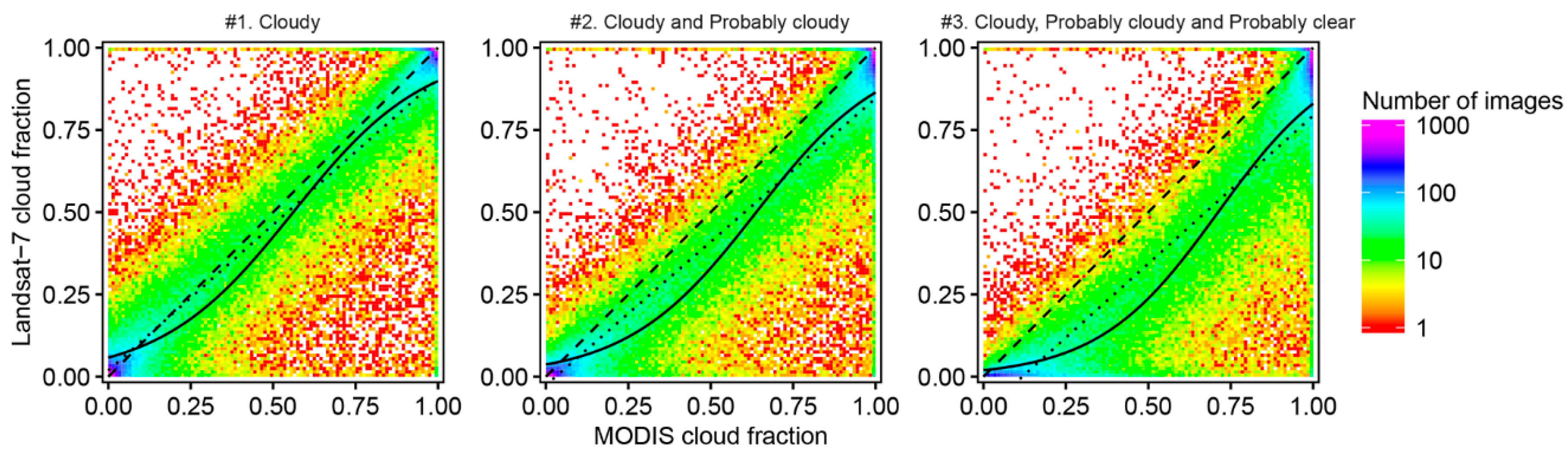
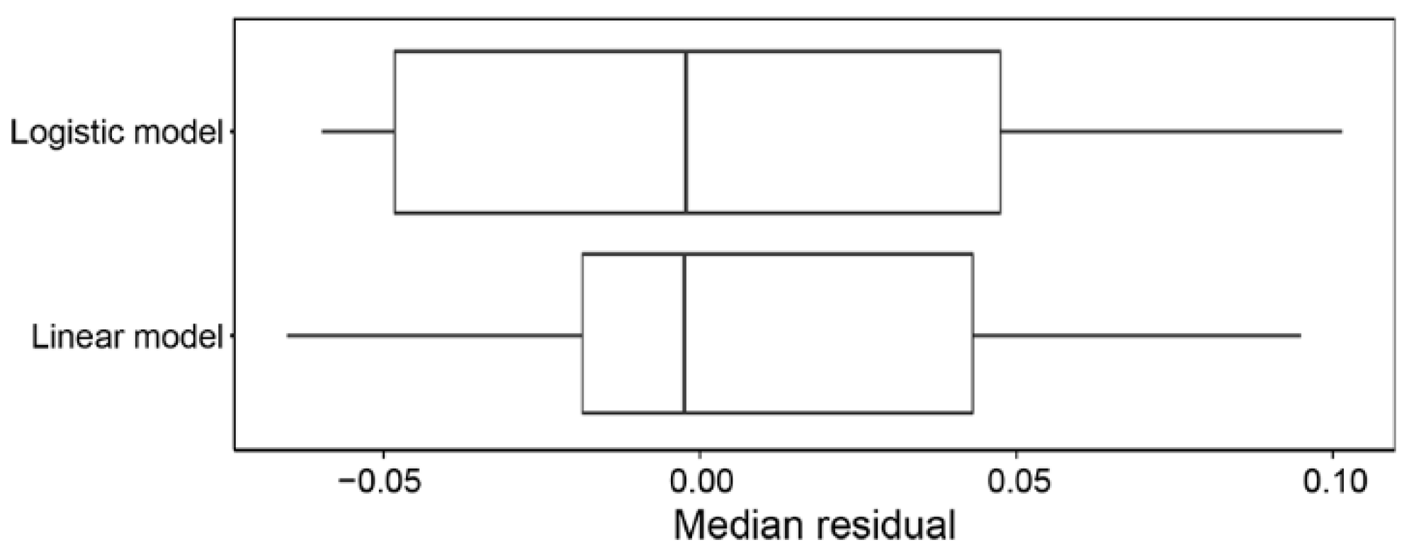
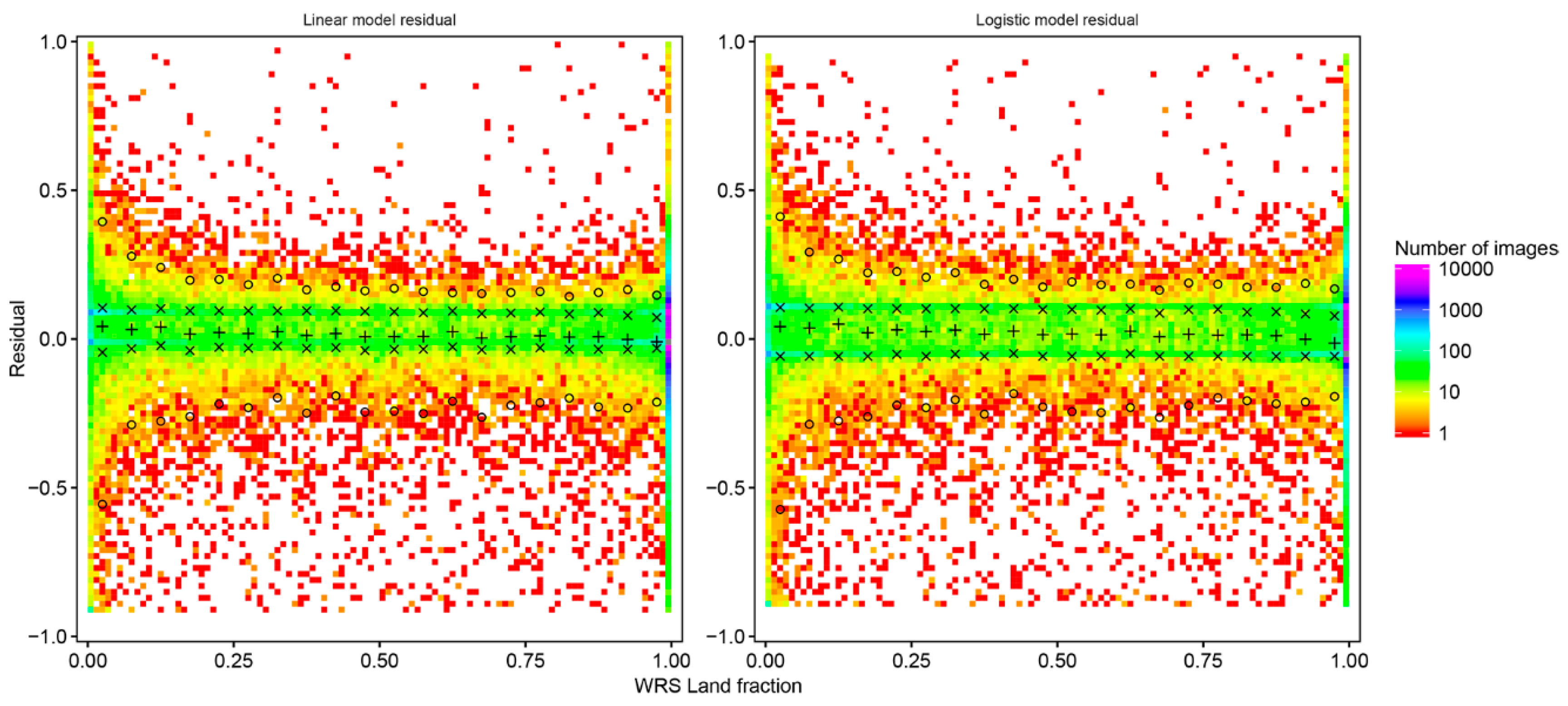
4.3. Regression Analysis

Figure 4 shows scatterplots comparing the Landsat 7 cloud fractions and the MODIS cloud fractions for the three MODIS cloud fraction definitions, and considers all the study data. The point density distribution, calculated using a 100 × 100 quantization of the axes, is plotted using a rainbow color scale. Linear and logistic regressions are shown plotted as dotted and continuous lines respectively. The correlation and regression coefficients are summarized in

Table 2. Regression results of the Landsat 7 and MODIS cloud fraction scatterplots shown in Figure 4.

	Definition	Coefficients	Standard Error of the Coefficients	Standard Error of the Residuals	R2	p-Value
Linear	#1	β0: 0.02, β1: 0.89	β0: 0.0007, β1: 0.0012	0.149	0.83	<2^−16
Model	#2	β0: −0.02, β1: 0.87	β0: 0.0008, β1: 0.0012	0.157	0.82	<2^−16
	#3	β0: −0.10, β1: 0.90	β0: 0.0011, β1: 0.0016	0.186	0.74	<2^−16
	Definition	Coefficients	Standard Error of the Coefficients	Residual Deviance	Null Deviance	p-Value
Logistic	#1	β0: −2.79, β1: 4.97	β0: 0.016, β1: 0.026	18,194	76,678	<2^−16
Model	#2	β0: −3.26, β1: 5.11	β0: 0.019, β1: 0.027	18,199	76,678	<2^−16
	#3	β0: −3.91, β1: 5.50	β0: 0.023, β1: 0.031	22,146	76,678	<2^−16

. Consistent with the boxplot results presented in Figure 3, the scatterplots indicate that the MODIS cloud fraction is closest to the Landsat cloud fractions when the most conservative MODIS cloud fraction definition is used (#1). Generally, MODIS overestimates the cloud fraction compared to Landsat and there is a progressive overestimation from definition #1 to #3, as shown by the majority of the point distribution (green to purple colors) positioned below the identity line (dashed line) for #2 and #3. This is also reflected by the linear regression lines: the regression lines of #2 and #3 are noticeably further apart from the identity line than the regression line for #1.

The logistic regression results are consistent with the results of the linear regression, with a similar residual deviance for definitions #1 (18,194) and #2 (18,199) and considerably higher residual deviance for #3 (22,146). For all three MODIS cloud definitions, the residual deviance is considerably smaller than the null deviance, indicating that the MODIS cloud fraction is an effective predictor for the Landsat 7 cloud fraction. For all three MODIS cloud definitions, the standard errors of the coefficients are smaller than the estimated values of the coefficients, and the regressions are significant (p < 0.05).

For all three MODIS cloud definitions, the linear regressions between the MODIS and the Landsat 7 cloud fractions are significant (p < 0.05). The highest coefficient of determination (R²) is observed for MODIS cloud definition #1 (R² = 0.83), with a progressively lower coefficient of determination for definition #2 (R² = 0.82) and #3 (R² = 0.74). While the β₁ (slope) coefficient is similar in the three definitions, with values of 0.89 (#1), 0.87 (#2) and 0.90 (#3), the β₀ (intercept) coefficient decreases from 0.02 (#1), to −0.02 (#2) and −0.10 (#3), reflecting that the MODIS cloud fractions become systematically higher than the Landsat cloud fractions when the less conservative cloud definitions #2 and #3 are considered. The standard error of the residuals is also lower for definition #1 (0.149) compared to #2 (0.157) and #3 (0.186).

To further investigate the behavior of the linear and logistic models, the regression residuals, i.e., the observed minus the predicted Landsat 7 cloud fractions, are summarized in Figure 5 for the global year of study data. The scatter plots in Figure 5 were obtained by plotting the regression residuals as a function of the MODIS cloud fraction. The scatter plots separately consider the linear (top row) and logistic models (bottom row), for MODIS cloud definitions #1 (left column), #2 (center column) and #3 (right column). In all plots, the majority of the data points (green to purple colors) corresponds to low residuals (i.e., y-axes values close to 0), and only isolated data points (red colors) correspond to large residuals (up to 1.0 and −1.0). Consistent with the results of Figure 4 and Table 2, the most conservative MODIS cloud fraction definition (#1) has residuals that are clustered around 0 on the y-axes, whereas definitions #2 and #3 have more dispersed residuals.

The median (denoted by + symbols) and interquartile range (x symbols) of the residuals over four subdivisions of the MODIS cloud fraction range from [0, 0.25], [0.25, 0.50], [0.5, 0.75], and [0.75, 1] and are shown in Figure 5. These four ranges are used to broadly verify whether the distribution of the residuals changes as a function of the MODIS cloud fraction, i.e., to identify any potential heteroscedasticity of the data, which would violate some of the underlying assumptions of the regression analyses. The residual median and interquartile range values do not significantly change across the MODIS cloud fraction range, indicating that no marked heteroscedasticity is present for both the linear and logistic models, and for any of the three MODIS cloud mask definitions.

The most conservative MODIS cloud fraction definition (#1) has the highest linear regression R², and lowest logistic regression residual deviance (Table 2).

Table 3. Median, 25th and 75th quantiles of the residuals for the linear (top) and logistic (bottom) models. The residuals were calculated globally and divided in MODIS definition #1 cloud fraction intervals.

Linear Model	MODIS Cloud Definition #1 Cloud Fraction Interval
Residual value	[0, 0.25]	[0.25, 0.50]	[0.50, 0.75]	[0.75, 1]	[0, 1]
25th quantile	−0.022	−0.097	−0.100	−0.007	−0.032
Median	−0.018	−0.005	0.004	0.077	−0.003
75th quantile	0.015	0.079	0.084	0.096	0.085
Logistic Model	MODIS Cloud Definition #1 CLOUD Fraction Interval
Residual value	[0, 0.25]	[0.25, 0.50]	[0.50, 0.75]	[0.75, 1]	[0, 1]
25th quantile	−0.058	−0.036	−0.105	−0.031	−0.058
Median	−0.047	0.057	−0.001	0.062	−0.003
75th quantile	0.019	0.142	0.079	0.101	0.091

summarizes for this definition the median and interquartile range of the residuals for both regressions. The linear model has lower residuals than the logistic model for very low cloud fraction (<0.25), but slightly higher residuals at higher cloud fraction; overall, however, the two models have similar performance, with identical value of the median error (−0.003 linear and logistic) and comparable interquartile ranges ([−0.032, 0.085] linear model, [−0.058, 0.091] logistic model). Thus, the most conservative MODIS cloud fraction definition (#1) is an effective predictor of the Landsat 7 cloud fraction, both when fitting a linear and a logistic model.

Figure 6 shows the geographic distribution of the minimum (top row), median (middle row) and maximum (bottom row) residuals for the linear (left column) and logistic (right column) regression using the most conservative MODIS cloud definition (#1). Negative residuals (red, yellow colors) indicate that the linear and logistic models overestimate the observed Landsat cloud fraction, whereas positive residuals (cyan and blue colors) indicate the linear and logistic models underestimate the Landsat cloud fraction. Large minimum and maximum residuals (top and bottom row) are predominantly observed at WRS path/rows locations over coastlines, or at high latitude, or over snow prone mountain ranges. This is discussed further in Section 5.

The minimum and maximum residual values are driven by outliers whereas the median values correspond to the 50th percentile of the residual distribution and are robust to outliers; as indicated by the prevalence of green colors in the Figure 6 middle row figures, the median of the residuals is close to 0 at most locations. This is further illustrated by Figure 7, which summarizes the distribution of the median residuals shown in the middle row of Figure 6. The global median residual is slightly negative (−0.002 in both models), with a small interquartile range ([−0.019; 0.043] for the linear model, [−0.048; 0.047] for the logistic model) and small 5th–95th quantile range ([−0.065; 0.095] for the linear model, [−0.060, 0.101] for the logistic model). This indicates that, while large median residuals occasionally occur, the most conservative MODIS cloud fraction definition (#1) is usually an effective predictor of the median Landsat 7 cloud fraction not only globally, but also at each WRS path/row location.

Figure 8 shows scatterplots of the linear and logistic regression residuals as a function of the land fraction in each Landsat image. The median, interquartile range and 5th–95th quantile range of the distribution summarize the distribution of the residuals. The residual median and interquartile ranges are stable, albeit with a small positive median residual (0.042 with both models) at small land fractions (0 to 0.05), and a small negative median residual (−0.009 linear, −0.014 logistic) for large land fractions (0.95 to 1.00). Consistent with Figure 6, the 5th−95th quantile range indicates that at small land fractions (0 to 0.05) there are large outliers in the residuals (range [−0.556, 0.394] linear, [−0.573, 0.412] logistic). The 5th−95th quantile range, however, drops quickly as the land fraction increases, and it remains substantially stable for land fractions >0.25.

Finally, in order to verify the presence of seasonal pattern, Figure 9 shows the residuals of the linear (top row) and logistic (bottom row) models as function of the acquisition date for the Landsat images in the northern (left column) and southern (right column) hemispheres. Median, interquartile range, and 5th–95th quantile ranges of the residuals are plotted for quarterly intervals, defined as {[January–March], [April–June], [July–September], [October–December]}, and are summarized in

Table 4. Median, 5th, 25th, 75th and 95th quantiles of the residuals for the linear (top) and logistic (bottom) models. The residuals were calculated globally and divided in quarterly acquisition date intervals.

			Acquisition Date Interval
			Jan–Mar	Apr–Jun	Jul–Sep	Oct–Dec	Year
Linear model	Northern Hemisphere	5th quantile	−0.394	−0.217	−0.161	−0.264	−0.258
		25th quantile	−0.086	−0.036	−0.020	−0.044	−0.038
		Median	−0.019	0.002	0.020	−0.009	0.001
		75th quantile	0.079	0.089	0.095	0.081	0.089
		95th quantile	0.180	0.172	0.175	0.164	0.173
	Southern Hemisphere	5th quantile	−0.170	−0.172	−0.147	−0.154	−0.159
		25th quantile	−0.022	−0.019	−0.019	−0.022	−0.020
		Median	0.005	−0.015	−0.016	−0.008	−0.009
		75th quantile	0.088	0.054	0.053	0.071	0.069
		95th quantile	0.174	0.163	0.158	0.152	0.161
Logistic model	Northern Hemisphere	5th quantile	−0.390	−0.205	−0.150	−0.251	−0.244
		25th quantile	−0.073	−0.058	−0.049	−0.058	−0.058
		Median	−0.030	0.008	0.027	−0.012	0.003
		75th quantile	0.085	0.095	0.101	0.087	0.094
		95th quantile	0.192	0.189	0.197	0.184	0.192
	Southern Hemisphere	5th quantile	−0.164	−0.165	−0.129	−0.141	−0.150
		25th quantile	−0.058	−0.058	−0.058	−0.058	−0.058
		Median	0.004	−0.034	−0.038	−0.012	−0.021
		75th quantile	0.093	0.063	0.062	0.079	0.075
		95th quantile	0.201	0.191	0.186	0.178	0.188

.

While no seasonal pattern is detected in the Southern Hemisphere, in the Northern Hemisphere the residuals exhibit a slight seasonal pattern, with higher residual in the winter months. The median of the residuals changes from 0.020 (linear) and 0.027 (logistic) in July–September to −0.019 (linear) and −0.030 (logistic) in January–March. Furthermore, while the 25th, 75th and 95th quantile are substantially stable, the 5th percentile shows the largest seasonal trend, with a variation from −0.161 (linear) and −0.150 (logistic) in July−September to −0.394 (linear) and −0.390 (logistic). These results indicate that the large minimum residuals at high latitude shown in Figure 6, (top row), are predominantly observed on images acquired in the Northern Hemisphere in January–March, i.e., in the winter months.

5. Discussion

Linear and logistic models were used to predict the Landsat 7 ETM+ cloud fraction from MODIS MOD35 observations, and a non-parametric analysis of the residuals was performed. Overall, the analysis indicates a high degree of correspondence between the Landsat and MODIS cloud fractions, with the best results observed when only the pixels confidently labeled as cloudy in the MOD35 product are used. This case resulted in the highest coefficient of determination and lowest residuals, when fitting the linear and the logistic models. The difference between the MODIS and Landsat cloud fractions increases when less conservative MOD35 cloud definitions are used, i.e., when MODIS pixels flagged as potentially cloudy and potentially clear are counted in the cloud fraction. Arguably, this can be explained considering that the MOD35 cloud masking algorithm makes use of the multiple thermal bands and the water vapor/CO₂ absorption bands which are available on the MODIS instrument. These bands are missing from the Landsat ETM+ instrument, resulting in low sensitivity to thin clouds [28].

The analysis of the residuals indicates that the performance of the linear and logistic models were substantially similar, with the linear model marginally better at low cloud fraction conditions, and the logistic model marginally better for higher cloud fraction conditions. In the case of the linear model, the intercept of the regression line is small (0.02), the slope is close to unity (0.87), and the median of the residuals is also small (−0.002); this small positive error indicates that the use of MODIS to predict the Landsat cloud fraction results in a small overestimation of the cloud cover. With either model, the MODIS-Terra cloud mask underestimates the Landsat cloud fraction at low cloud levels, and overestimates it at high cloud levels. Arguably this is due to the MODIS coarse resolution: small, sparse clouds are not detected, and similarly small gaps in cloud cover are missed. These findings are consistent with previous studies reporting that the MODIS cloud masking algorithm results in some degree of overestimation on fragmented and optically thin clouds [18,21]. Further, this is a well-known scale issue whereby coarse resolution detection products tend to over and underestimate the area detected, compared to higher resolution products, when the areal proportions being detected are high and low respectively. For example, this has been observed in comparison of MODIS and Landsat derived burned areas [36], snow cover [37], and comparison of AVHRR and Landsat derived forest maps [38].

The geographic analysis of the residuals revealed that the largest differences between the MODIS and Landsat cloud fraction occur along the coastlines, and at high latitude. In the case of coastal areas, further analysis indicated that the errors are mostly observed at WRS path/row locations with land fractions ≤0.05. In these cases, cloud movement in the 30 minutes between the MODIS-Terra and Landsat 7 overpasses may result in large discrepancies of the estimated cloud percentage over land. Furthermore, false positives in the MOD35 cloud mask over coastlines, rivers and lake regions are known issues of the MOD35 product [10,39]. Additionally, the temporal analysis of the residuals showed the presence of a seasonal effect in the Northern Hemisphere: the overestimation of the Landsat cloud fraction by the MODIS cloud mask is greater in winter than in summer. Visual inspection of the MODIS and Landsat images, where large discrepancies were observed, confirmed that, at high latitudes and over mountain ranges, ice and snow were flagged as clouds by the MODIS MOD35 product, also a known issue of the MOD35 product [10,40,41].

The results of this study indicate that the MODIS-Terra 1 km cloud product can be used to predict Landsat 7 ETM+ image cloud fractions over land. Thus, the consistent, long term (2000 onwards) daily cloud observations from the MODIS-Terra instrument can be used to assess the impact of cloud on moderate resolution land monitoring products from the Landsat satellites. Recommendations for the next (after Landsat 9) mission design are currently being developed [3]. Due to the high cost of thermal wavelength sensors, a possible design option may be to have separate satellites carrying thermal infrared (TIR) and visible to shortwave infrared wavelength (VSWIR) detectors. The degree of temporal overpass separation between the TIR and the VSWIR observations will be considered in application specific terms, but also to minimize overpass cloudiness differences. The results of this study indicate that, in the morning sun-synchronous orbit, an approximately 30 minute overpass time difference does not, globally on average, result in significant differences in observed cloud fraction over land. We finally note that some cautions must be used in considering these results, as high residuals of the linear and logistic regression models were observed on individual images, especially in the presence of snow or on coastal areas.

6. Conclusions

In this paper, a systematic global comparison between the Landsat 7 ETM+ image cloud fraction over land, and equivalent cloud fractions derived from contemporaneous MODIS-Terra (MOD35) cloud observations was undertaken. Three MODIS cloud fraction definitions were considered, including a conservative cloud definition, an intermediated definition and a much less conservative definition. Due to the similar acquisition orbits and overpass times, the MODIS MOD35 global cloud mask product is a good predictor of the Landsat 7 ETM+ image cloud fraction over land. The most conservative MODIS cloud fraction definition was the best predictor of the Landsat 7 ETM+ cloud fraction, resulting in high coefficient of determination (R² = 0.83), negligible bias (median difference: <0.01) and low dispersion around the median (interquartile range: [−0.02, 0.06]) of the estimated linear model. These results suggest that it is possible to use the daily probability of cloud cover, as observed by MODIS-Terra, as a proxy of the cloud cover observed by Landsat 7.

References

1. Roy, D.P.; Wulder, M.A.; Loveland, T.R.; Woodcock, C.E.; Allen, R.G.; Anderson, M.C.; Helder, D.; Irons, J.R.; Johnson, D.M.; Kennedy, R.; et al. Landsat-8: Science and product vision for terrestrial global change research. Remote Sens. Environ. 2014, 145, 154–172. [Google Scholar] [CrossRef] [Green Version]
2. Drusch, M.; Del Bello, U.; Carlier, S.; Colin, O.; Fernandez, V.; Gascon, F.; Hoersch, B.; Isola, C.; Laberinti, P.; Martimort, P. Sentinel-2: ESA’s optical high-resolution mission for GMES operational services. Remote Sens. Environ. 2012, 120, 25–36. [Google Scholar] [CrossRef]
3. Wulder, M.A.; Loveland, T.R.; Roy, D.P.; Crawford, C.J.; Masek, J.G.; Woodcock, C.E.; Allen, R.G.; Anderson, M.C.; Belward, A.S.; Cohen, W.B.; et al. Current status of Landsat program, science, and applications. Remote Sens. Environ. 2019, 225, 127–147. [Google Scholar] [CrossRef]
4. Li, J.; Roy, D. A global analysis of Sentinel-2a, Sentinel-2b and Landsat-8 data revisit intervals and implications for terrestrial monitoring. Remote Sens. 2017, 9, 902. [Google Scholar]
5. Boschetti, L.; Roy, D.P.; Justice, C.O.; Humber, M.L. MODIS–Landsat fusion for large area 30 m burned area mapping. Remote Sens. Environ. 2015, 161, 27–42. [Google Scholar] [CrossRef]
6. Melchiorre, A.; Boschetti, L. Global analysis of burned area persistence time with MODIS data. Remote Sens. 2018, 10, 750. [Google Scholar] [CrossRef] [Green Version]
7. Roy, D.P.; Huang, H.; Boschetti, L.; Giglio, L.; Yan, L.; Zhang, H.H.; Li, Z. Landsat-8 and Sentinel-2 burned area mapping—A combined sensor multi-temporal change detection approach. Remote Sens. Environ. 2019, 231, 111254. [Google Scholar] [CrossRef]
8. Pekel, J.-F.; Cottam, A.; Gorelick, N.; Belward, A.S. High-resolution mapping of global surface water and its long-term changes. Nature 2016, 540, 418. [Google Scholar] [CrossRef] [PubMed]
9. Roy, D.P.; Yan, L. Robust landsat-based crop time series modelling. Remote Sens. Environ. 2018. [Google Scholar] [CrossRef]
10. Ackerman, S.; Strabala, K.; Menzel, P.; Frey, R.; Moeller, C.; Gumley, L. Discriminating Clear-Sky from Cloud with MODIS Algorithm Theoretical Basis Document (MOD35) Version 6.1; Cooperative Institute for Meteorological Satellite Studies, University of Wisconsin—Madison: Madison, WI, USA, 2010. [Google Scholar]
11. Whitcraft, A.; Becker-Reshef, I.; Killough, B.; Justice, C. Meeting earth observation requirements for global agricultural monitoring: An evaluation of the revisit capabilities of current and planned moderate resolution optical earth observing missions. Remote Sens. 2015, 7, 1482–1503. [Google Scholar] [CrossRef] [Green Version]
12. Wulder, M.A.; White, J.C.; Loveland, T.R.; Woodcock, C.E.; Belward, A.S.; Cohen, W.B.; Fosnight, E.A.; Shaw, J.; Masek, J.G.; Roy, D.P. The global Landsat archive: Status, consolidation, and direction. Remote Sens. Environ. 2016, 185, 271–283. [Google Scholar] [CrossRef] [Green Version]
13. Mercury, M.; Green, R.; Hook, S.; Oaida, B.; Wu, W.; Gunderson, A.; Chodas, M. Global cloud cover for assessment of optical satellite observation opportunities: A HyspIRI case study. Remote Sens. Environ. 2012, 126, 62–71. [Google Scholar] [CrossRef]
14. Whitcraft, A.K.; Vermote, E.F.; Becker-Reshef, I.; Justice, C.O. Cloud cover throughout the agricultural growing season: Impacts on passive optical earth observations. Remote Sens. Environ. 2015, 156, 438–447. [Google Scholar] [CrossRef]
15. Goward, S.N.; Loboda, T.V.; Williams, D.L.; Huang, C. Landsat orbital repeat frequency and cloud contamination: A case study for eastern united states. Photogramm. Eng. Remote Sens. 2019, 85, 109–118. [Google Scholar] [CrossRef]
16. Feidas, H.; Cartalis, C. Application of an automated cloud-tracking algorithm on satellite imagery for tracking and monitoring small mesoscale convective cloud systems. Int. J. Remote Sens. 2005, 26, 1677–1698. [Google Scholar] [CrossRef]
17. Li, Z.; Roy, D.P.; Zhang, H.K.; Vermote, E.F.; Huang, H. Evaluation of Landsat-8 and Sentinel-2a aerosol optical depth retrievals across Chinese cities and implications for medium spatial resolution urban aerosol monitoring. Remote Sens. 2019, 11, 122. [Google Scholar] [CrossRef] [Green Version]
18. King, M.D.; Platnick, S.; Menzel, W.P.; Ackerman, S.A.; Hubanks, P.A. Spatial and temporal distribution of clouds observed by MODIS onboard the terra and aqua satellites. IEEE Trans. Geosci. Remote Sens. 2013, 51, 3826–3852. [Google Scholar] [CrossRef]
19. Roy, D.; Lewis, P.; Schaaf, C.; Devadiga, S.; Boschetti, L. The global impact of clouds on the production of modis bidirectional reflectance model-based composites for terrestrial monitoring. IEEE Geosci. Remote Sens. Lett. 2006, 3, 452–456. [Google Scholar] [CrossRef] [Green Version]
20. Hagihara, Y.; Okamoto, H.; Yoshida, R. Development of a combined CloudSat-CALIPSO cloud mask to show global cloud distribution. J. Geophys. Res. Atmos. 2010, 115. [Google Scholar] [CrossRef] [Green Version]
21. Zhao, G.; Di Girolamo, L. Cloud fraction errors for trade wind cumuli from EOS-Terra instruments. Geophys. Res. Lett. 2006, 33. [Google Scholar] [CrossRef]
22. Ackerman, S.A.; Strabala, K.I.; Menzel, W.P.; Frey, R.A.; Moeller, C.C.; Gumley, L.E. Discriminating clear sky from clouds with MODIS. J. Geophys. Res. Atmos. 1998, 103, 32141–32157. [Google Scholar] [CrossRef]
23. Holz, R.; Ackerman, S.; Nagle, F.; Frey, R.; Dutcher, S.; Kuehn, R.; Vaughan, M.; Baum, B. Global Moderate Resolution Imaging Spectroradiometer (MODIS) cloud detection and height evaluation using CALIOP. J. Geophys. Res. Atmos. 2008, 113. [Google Scholar] [CrossRef] [Green Version]
24. Foga, S.; Scaramuzza, P.L.; Guo, S.; Zhu, Z.; Dilley, R.D.; Beckmann, T.; Schmidt, G.L.; Dwyer, J.L.; Joseph Hughes, M.; Laue, B. Cloud detection algorithm comparison and validation for operational Landsat data products. Remote Sens. Environ. 2017, 194, 379–390. [Google Scholar] [CrossRef] [Green Version]
25. Chander, G.; Xiong, X.; Choi, T.; Angal, A. Monitoring on-orbit calibration stability of the Terra MODIS and Landsat 7 ETM+ sensors using pseudo-invariant test sites. Remote Sens. Environ. 2010, 114, 925–939. [Google Scholar] [CrossRef]
26. Goward, S.N.; Masek, J.G.; Williams, D.L.; Irons, J.R.; Thompson, R. The Landsat 7 mission: Terrestrial research and applications for the 21st century. Remote Sens. Environ. 2001, 78, 3–12. [Google Scholar] [CrossRef]
27. Arvidson, T.; Gasch, J.; Goward, S.N. Landsat 7’s long-term acquisition plan—An innovative approach to building a global imagery archive. Remote Sens. Environ. 2001, 78, 13–26. [Google Scholar] [CrossRef]
28. Zhu, Z.; Woodcock, C.E. Object-based cloud and cloud shadow detection in Landsat imagery. Remote Sens. Environ. 2012, 118, 83–94. [Google Scholar] [CrossRef]
29. Zhu, Z.; Wang, S.; Woodcock, C.E. Improvement and expansion of the Fmask algorithm: Cloud, cloud shadow, and snow detection for Landsats 4–7, 8, and Sentinel 2 images. Remote Sens. Environ. 2015, 159, 269–277. [Google Scholar] [CrossRef]
30. Wolfe, R.E.; Roy, D.P.; Vermote, E. MODIS land data storage, gridding, and compositing methodology: Level 2 grid. IEEE Trans. Geosci. Remote Sens. 1998, 36, 1324–1338. [Google Scholar] [CrossRef] [Green Version]
31. Masuoka, E.; Fleig, A.; Wolfe, R.E.; Patt, F. Key characteristics of MODIS data products. IEEE Trans. Geosci. Remote Sens. 1998, 36, 1313–1323. [Google Scholar] [CrossRef]
32. Wolfe, R.E.; Nishihama, M.; Fleig, A.J.; Kuyper, J.A.; Roy, D.P.; Storey, J.C.; Patt, F.S. Achieving sub-pixel geolocation accuracy in support of MODIS land science. Remote Sens. Environ. 2002, 83, 31–49. [Google Scholar] [CrossRef]
33. Markham, B.L.; Storey, J.C.; Williams, D.L.; Irons, J.R. Landsat sensor performance: History and current status. IEEE Trans. Geosci. Remote Sens. 2004, 42, 2691–2694. [Google Scholar] [CrossRef]
34. Kovalskyy, V.; Roy, D.P. The global availability of Landsat 5 TM and Landsat 7 ETM+ land surface observations and implications for global 30 m Landsat data product generation. Remote Sens. Environ. 2013, 130, 280–293. [Google Scholar] [CrossRef] [Green Version]
35. Ju, J.; Roy, D.P. The availability of cloud-free Landsat ETM+ data over the conterminous United States and globally. Remote Sens. Environ. 2008, 112, 1196–1211. [Google Scholar] [CrossRef]
36. Roy, D.P.; Boschetti, L. Southern Africa validation of the MODIS, L3JRC, and GlobCarbon burned-area products. IEEE Trans. Geosci. Remote Sens. 2009, 47, 1032–1044. [Google Scholar] [CrossRef]
37. Hall, D.K.; Riggs, G.A. Accuracy assessment of the MODIS snow products. Hydrol. Process. 2007, 21, 1534–1547. [Google Scholar] [CrossRef]
38. Mayaux, P.; Lambin, E.F. Tropical forest area measured from global land-cover classifications: Inverse calibration models based on spatial textures. Remote Sens. Environ. 1997, 59, 29–43. [Google Scholar] [CrossRef]
39. Ault, T.W.; Czajkowski, K.P.; Benko, T.; Coss, J.; Struble, J.; Spongberg, A.; Templin, M.; Gross, C. Validation of the MODIS snow product and cloud mask using student and NWS cooperative station observations in the lower great lakes region. Remote Sens. Environ. 2006, 105, 341–353. [Google Scholar] [CrossRef]
40. Li, Z.; Cribb, M.; Chang, F.; Trishchenko, A. Validation of MODIS-retrieved cloud fractions using whole sky imager measurements at the three arm sites. In Proceedings of the 14th ARM Science Team Meeting, Albuquerque, NM, USA, 22–26 March 2004; pp. 1–6. [Google Scholar]
41. Stillinger, T.; Roberts, D.A.; Collar, N.M.; Dozier, J. Cloud masking for Landsat 8 and MODIS Terra over snow-covered terrain: Error analysis and spectral similarity between snow and cloud. Water Resour. Res. 2019, 55, 6169–6184. [Google Scholar] [CrossRef] [Green Version]
Figure 1. Spatial distribution and number of Landsat 7 ETM+ images acquired from 1 January to 31 December 2002 between 70°S and 70°N. The number of images for each Landsat WRS path/row is depicted with a rainbow color scale.
Remotesensing 12 00202 g001
Figure 2. Histograms of Landsat 7 (top) and MODIS (bottom row) cloud fractions, observed in all the 2002 study data (Figure 1). The histograms are quantized using 100 bins of equal width. The three MODIS cloud fraction histograms are for the three MODIS cloud definitions (Table 1).
Remotesensing 12 00202 g002
Figure 3. Box and whisker plots summarizing the distribution of the difference between the MODIS and Landsat 7 cloud fractions for all the global 2002 data (Figure 1) considering the three MODIS cloud fraction definitions (Table 1). The thick vertical lines show the median of the distribution, the boxes show the interquartile range, and the whiskers show the 5th to 95th quartile range.
Remotesensing 12 00202 g003
Figure 4. Scatterplot of the Landsat 7 cloud fraction plotted against the MODIS cloud fraction, considering all the 2002 study data, plotted for each MODIS cloud fraction definition (Table 1). The logistic regression (solid), linear regression (dotted) and the identity line (dashed) are shown superimposed on point density distributions that are generated using a 100 × 100 quantization of the axes, and are displayed with a rainbow logarithmic color scale.
Remotesensing 12 00202 g004
Figure 5. Scatterplot of the regression model residuals, defined as the observed minus the predicted Landsat 7 cloud fraction, plotted against the MODIS cloud fraction for the linear (top row) and the logistic regression model (bottom row) considering the 3 MODIS cloud fraction definitions (Table 1). The median (+) and interquartile range (x) of the residuals are shown for four MODIS cloud fraction bins: [0, 0.25], [0.25, 0.50], [0.5, 0.75], and [0.75, 1].
Remotesensing 12 00202 g005
Figure 6. Spatial distribution of the minimum (top row), median (middle row) and maximum (bottom row) residuals observed at each WRS path/row location for the linear (left column) and logistic (right column) regression using the most conservative MODIS cloud definition (#1). The residuals are depicted using the same rainbow color scale for easier comparison.
Remotesensing 12 00202 g006
Figure 7. Box and whisker plots summarizing the distribution of the median residual of the linear and logistic models at each WRS path/row location (i.e., Figure 6, middle row). The thick vertical lines show the median of the distribution, the boxes show the interquartile range, and the whiskers show the 5th–95th quantile range.
Remotesensing 12 00202 g007
Figure 8. Scatterplot of the linear (left) and logistic (right) regression residuals plotted against the land fraction in each Landsat path/row, considering all the 2002 study data, for the most conservative MODIS cloud fraction definition (#1). The median (+), interquartile range (x) and 5th−95th quantile range (°) of the residuals are shown for 0.05 land fraction bins. The point density distributions are generated using a 100 × 100 quantization of the axes, and are displayed with a rainbow logarithmic color scale.
Remotesensing 12 00202 g008
Figure 9. Scatterplot of the linear (top row) and logistic (bottom row) regression residuals divided between the northern (left column) and southern hemisphere (right column) plotted against the Landsat acquisition day of year, considering all the 2002 study data, plotted for the most conservative MODIS cloud fraction definition (#1) (Table 1). The point density distributions are generated using a 25 × 25 quantization of the axes, and are displayed with a rainbow logarithmic color scale. It should be noted that the artifact visible in all plots for days 75−90 is due to a gap from March 19th to 28th in the MODIS-Terra data acquisition. The median (+), interquartile range (x) and the 5th−95th quantile range (°) of the residuals are shown for quarterly acquisition intervals, defined as {[Jan−Mar], [Apr−Jun], [Jul−Sep], [Oct−Dec]}.
Remotesensing 12 00202 g009