Article

Testing Side-Scan Sonar and Multibeam Echosounder to Study Black Coral Gardens: A Case Study from Macaronesia

by
Karolina Czechowska
1,†,
Peter Feldens
2,†,
Fernando Tuya
1,
Marcial Cosme de Esteban
1,
Fernando Espino
1,
Ricardo Haroun
1,
Mischa Schönke
2 and
Francisco Otero-Ferrer
1,3,*,†
1
Grupo en Biodiversidad y Conservación (IU-ECOAQUA), Universidad de Las Palmas de Gran Canaria, 35200 Telde, Spain
2
Leibniz Institute for Baltic Sea Research Warnemünde (IOW), 18119 Warnemünde, Germany
3
Asociación Biodiversidad Atlántica y Sostenibilidad (ABAS), 25200 Telde, Spain
*
Author to whom correspondence should be addressed.
These authors contributed equally to this work.
Remote Sens. 2020, 12(19), 3244; https://doi.org/10.3390/rs12193244
Submission received: 11 September 2020 / Revised: 28 September 2020 / Accepted: 29 September 2020 / Published: 6 October 2020
(This article belongs to the Special Issue Remote Sensing of Islands)

Abstract

:
Black corals (order Antipatharia) are important components of mesophotic and deep-water marine communities, but due to their inaccessibility, there is limited knowledge about the basic aspects of their distribution and ecology. The aim of this study was to test methodologies to map and study colonies of a branched antipatharian species, Antipathella wollastoni, in the Canary Islands (Spain). Acoustic tools, side-scan sonar (SSS), and a multibeam echosounder (MBES), coupled with ground-truthing video surveys, were used to determine the habitat characteristics of Antipathella wollastoni. Below 40 m depth, colonies of increasing height (up to 1.3 m) and abundance (up to 10 colonies/m2) were observed, particularly on steep and current-facing slopes on rocky substrates. However, coral presence was not directly imaged on backscatter mosaics and bathymetric data. To improve this situation, promising initial attempts of detecting Antipathella wollastoni by utilizing the MBES water column scatter in an interval for 0.75 m to 1 m above the seafloor are reported.

1. Introduction

In the current Anthropocene era, human activities have put the natural world under unprecedented danger. The need to protect marine biodiversity is acknowledged by many international frameworks, such as the Convention on Biological Diversity and the Habitat and the Marine Strategy Framework Directives [1,2,3]. Information about the distribution and extent of marine habitats is critical for identifying and understanding species life-history traits, relationships between different ecosystems, and their resilience to anthropogenic impacts. Moreover, decision-making processes regarding management of living and non-living marine resources, e.g., fisheries and deep-sea mining, and marine spatial planning strategies require baseline data on the distribution of marine habitats [4,5,6,7,8]. Therefore, habitat mapping constitutes a vital first step for the sustainable management of the marine environment. The seabed has remained vastly undescribed because of financial, logistical, and technical challenges associated with studying ocean depths. Remote sensing technologies using sound propagation and detection are commonly used to map different seafloor and benthic habitats [9,10,11]. Exploring the possibilities and limitations of currently available tools is essential for their optimization for seabed mapping. Two commonly used techniques, side-scan sonar (SSS) and the multibeam echosounder (MBES), have already been deployed to detect and study shallow-water marine habitats, such as coral reefs [12], seagrass meadows [13], and rhodolith beds [14], but also deeper habitats, such as deep-water coral mounds [15,16,17]. Both tools emit sound beams narrow in the along-track direction that cover wide swathes of the seafloor perpendicular to the survey line and then record the sound scattered back [18]. For SSS techniques, two sideways-looking transducers send out two across-track broad sound beams, so the acoustic scatter properties of the seafloor (i.e., the backscatter intensity) are recorded at fixed time intervals. This way, SSS produces sideways profiles of the seabed, which can be used to visually differentiate between habitats based on their physical structure and terrain texture. Moreover, SSS can be towed behind a boat, so recording devices (the “fish”) are positioned close to the seafloor and can provide images of high resolution, even for deep seabeds [19]. However, the towing means that the geographic coordinates of the data acquired are less accurate due to current dragging of the towfish and a flat bottom assumption inherent in non-interferometric side-scan sonars [20,21]. Meanwhile, the MBES separates the across-track sound beams into 256–1024 separate beams and measures, apart from the backscatter intensity, the return and transmit angles for each beam, which enable the MBES to produce depth profiles. The MBES can be used to create detailed bathymetric maps, three-dimensional images of the seabed, and secondary data about terrain morphology, such as the slope, aspect (i.e., the azimuth direction that the slope faces), or rugosity (i.e., terrain variability). The seabed topography and structure can reveal dominant biological assemblages. In brief, terrain characteristics’ information, commonly included in ecological habitat suitability models, can be used as a proxy for the presence of biogenic habitats [9]. Both tools may be suited to detecting different seabed objects or may be complementary in their detection [22,23].
One of many marine habitats that remains understudied is the animal forests created by black corals [24]. Black corals belong to the order Antipatharia (phylum Cnidaria, class Anthozoa, subclass Hexacorallia), a group of ca. 250 species [25], which shows wide geographical and bathymetrical distribution, from polar to tropical latitudes [26] and from 2 m to 8.600 m depth, respectively [26,27]. In favorable environments, black corals may form dense, three-dimensional structures over large areas [24], which are categorized as “coral gardens” [28] (Figure 1). The black coral gardens are different from conventional coral reefs, as they have proteinaceous skeletons (no calcification process) and their colony morphologies vary from branched, bush-like, and feather-like to spiraled types [24]. By bringing diversification to the seafloor, creating habitats for associated faunal communities and changing local physical conditions, black corals act as “ecosystem engineers” [4,29,30]. Despite limited observations, black coral gardens can provide various ecosystem functions, particularly for faunal communities [31,32]: from the provision of habitat and shelter [33,34], food and feeding grounds [32,35,36,37], to nesting and nursery sites for commercial fish species [38] and deep-water invertebrates [39,40]. As other antipatharians, black corals show slow growth rates and extreme longevity [41,42,43], which make them vulnerable to anthropogenic threats, such as bottom fishing [30,44], illegal harvest for jewelery [45], mineral/gas/oil exploration, and construction of underwater pipelines [30,46]. To acknowledge their importance and threat status, they are classified as Vulnerable Marine Ecosystems (VMEs) by the United Nations General Assembly Resolutions 61/105 and 64/72 [47] and listed in the Appendix A of the Convention on International Trade in Endangered Species of Wild Fauna and Flora [48].
Black coral communities of Antipathella wollastoni [49] (Figure 1) have been reported to form extensive gardens in the Canarian archipelago, Spain [50], and nearby archipelagos in Macaronesia. Data about the distribution of A. wollastoni in the Canary Islands is scarce and mostly limited down to 50 m depth [51]. On the other hand, the Canary Islands, as other EU Outermost Regions, have experienced increasing trends of coastal development and tourism activities in the last few decades, with concomitant environmental pressures, which are likely to continue in the upcoming years. Moreover, the islands are under a high risk of heavy exploitation of marine resources (e.g., fishing, aquaculture, marine biotechnology, and ocean energy [52,53]). From the scarce information recorded, black coral gardens are localized close to the zones under human influences and major fishing areas [50,54]. Thus, it is critical to increase our understanding of these sensitive and understudied marine habitats to help policy-makers adapt their marine management and conservation programs. An efficient method of determining the spatial extension (and changes thereof) of black corals is essential to provide the basic information required for their conservation.
Therefore, the goal of this study was to test the feasibility of both SSS and the MBES to map and study A. wollastoni gardens. We expected that black coral branches, which approximately coincide with the acoustic wavelength for high-resolution SSS and the MBES, and colonies, which form dense aggregations, are likely to increase the acoustic scatter reported by these instruments. Therefore, although black corals do not form robust calcified mounds, they create a change in the physical structure of the seafloor that may be detected. Thus, we hypothesized that A. wollastoni gardens have a unique acoustic signature on backscatter data that reveals their presence and distribution in sonar surveys. Moreover, because substrate characteristics are important in determining species distribution, we hypothesized that seafloor morphology and structure information derived from sonar surveys can be used to describe and predict black coral habitats on a local scale. This study aims to increase the limited knowledge about the biological features of black coral gardens (A. wollastoni) off the Canary Islands, promoting much desired scientific research of these keystone mesophotic antipatharians occurring at depths of 25–100 m also in other subtropical eastern Atlantic archipelagos (e.g., Cape Verde, Madeira, and the Azores).

2. Materials and Methods
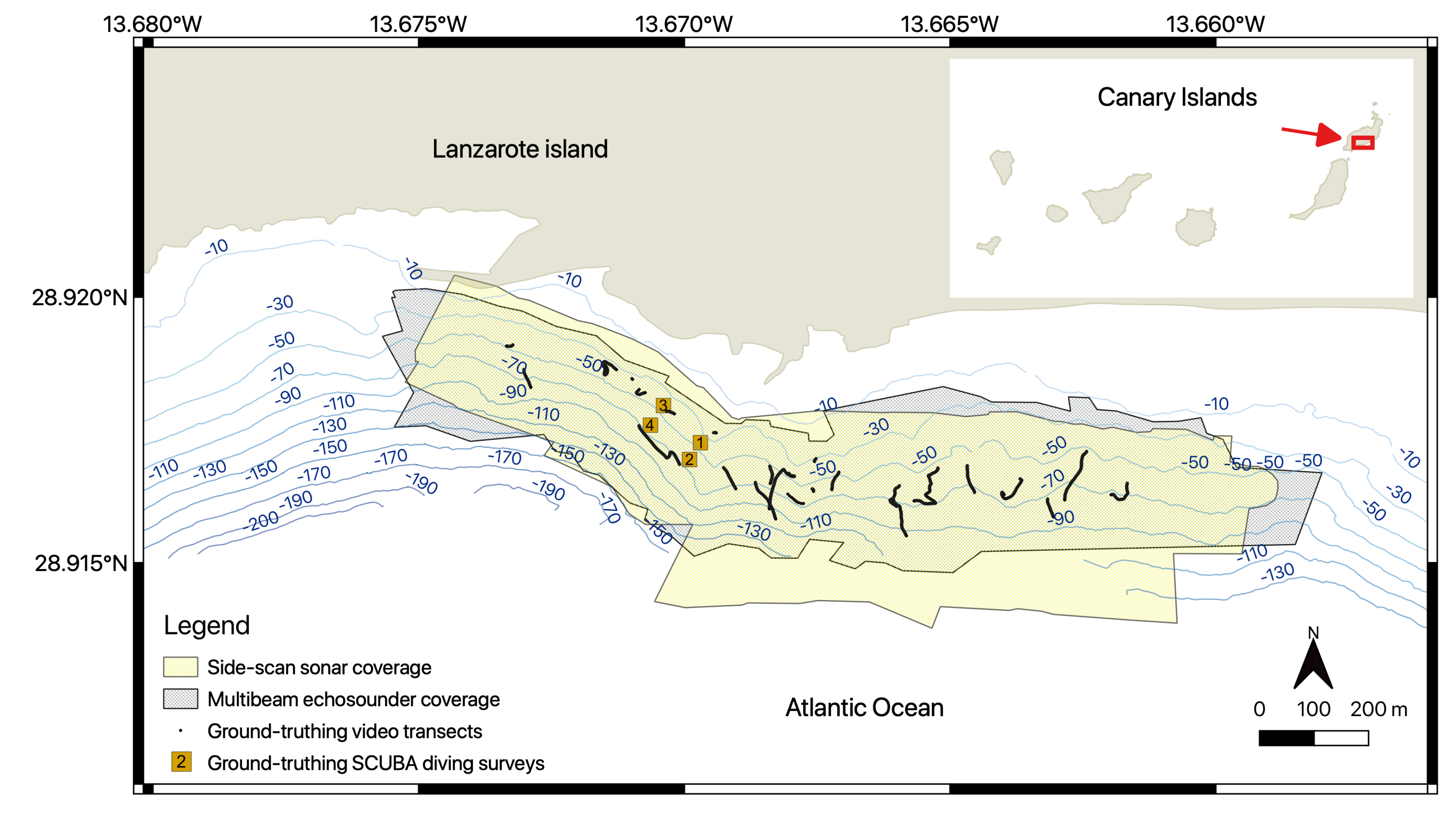
2.1. Study Site

The field work took place off the southeastern coast of Lanzarote Island (the Canary Islands, eastern Atlantic Ocean), outside Puerto del Carmen (28 55 5 N, 13 40 24 W; Figure 2). The site was selected on the basis of previous records of A. wollastoni in the shallower limits of its distribution (ca. 50 m depth [50]). Local topography is characterized by narrow rocky shelves and steep slopes, typical for oceanic volcanic islands [55,56]. Local hydrography is complex, with NE trade winds affecting shallow subtidal habitats by generating wind waves and near-bottom turbulence [57]. The high nutrient load transported by currents may affect the upper limit of black coral distribution, by either providing food or smothering the corals physically [24].

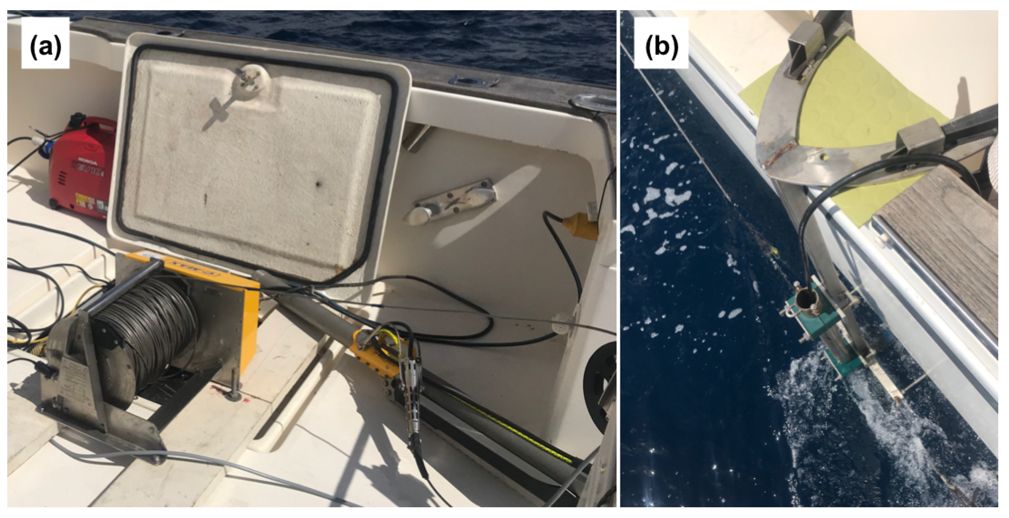
2.2. Hydroacoustic Data Acquisition

Hydroacoustic data were collected simultaneously with the side-scan sonar (SSS) and multibeam echosounder (MBES) techniques, using an 11 m fiberglass boat on 7–9 April 2019. Acoustic surveys were performed following the bathymetric profile (data available from Dirección General de Costas, Ministerio de Medio Ambiente, 2000), parallel to the coast, and covered ca. 55 ha and depths ranging ca. from 20 m to 150 m (Figure 2). The SSS, digital CM2 Towfish (C-Max, UK), was attached to a steel cable (Figure 3a) and towed behind the boat at a constant height from the sea bottom of ca. 20 m, with the vessel speed not exceeding 3.5 knots. The SSS was emitting signals with a central frequency of 325 kHz and an along-track horizontal beamwidth of 0.3 , covering a range of 100 m on both the port and starboard sides of the boat. The resolution of the mosaics is lowest in the along-track direction. Here, the resolution is given by the lower of Δ x = R × sin θ h , where R is the range and θ h the horizontal beamwidth [19], and the distance traveled by the boat between two successive pings, which is approximately 0.25 m. The SonarWiz 6 V6.05.0008 software (Chesapeake Technology Inc., Los Altos, CA, USA) acquired the backscatter data. A differential GPS, A325 GNSS Smart Antenna (Hemisphere, USA), was used for navigation and the SSS towfish positioning in the SonarWiz 6 software. The horizontal distance of the towfish behind the boat was obtained from the towing davit with the count cable pulley (CMAX Ltd., Dorset, UK), which calculated the amount of steel tow cable deployed. The SSS data were processed in SonarWiz 6 with empirical gain normalization, automatic gain control, beam angle correction, bottom tracking, layback correction, and the nadir filter.
The MBES, Norbit iWBMS Bathy (NORBIT, Norway), was attached to the port side of the boat at a depth of ca. 0.5 m with a custom-made metal mount (Figure 3b) and oriented vertically downwards. The MBES emitted signals with a central frequency of 400 kHz and an opening angle across the boat track of 100 –140 (depending on the water depth). The measurements were performed with a sweep time of 500 μ s, while the ping rate was controlled by the water depth. The Norbit iwbms software recorded the backscatter and depth values. An inertial navigation system, Applanix POS MV SurfMaster (Applanix, Richmond Hill, ON, Canada), provided position and motion compensation information. The sound velocity in the water was corrected using a sound velocity probe integrated into the MBES head. The MBES surveys recorded bathymetry in a depth range of 8.5 m to 173 m. However, the range with quality sufficient for visual interpretation was limited to ca. 120 m depth. The data processing required to create bathymetric and backscatter grids (i.e., pitch and roll calibration, automatic and manual removal of outliers, angular correction of intensity values and response curves to a reference angle of 40 ) was done using the open-source tool MB-System Version 5.5 (Caress and Chayes, 1995). Bathymetric data were processed to a resolution of 1 m. To obtain backscatter values, a low-pass filtered backscatter map of 2 m resolution was produced using MB-System to remove speckle noise. Darker areas in the produced map corresponded to weaker acoustic scatter intensities, while lighter areas to stronger acoustic scatter intensities in this study.
Information about the water column was extracted from snippet information recorded by the MBES. The Norbit system stores a 1 m long series of backscatter intensity both above and below the detected seafloor. Unfortunately, due to an unnoticed problem (a GPS antennae of the integrated Norbit system was shifted during camera retrieval and delivered the wrong information), data of sufficient quality exist only for a few ground-truthing video lines. A custom script was utilized to copy snippet information into the water column field of an s7k file (Version 3), with 2 fold downsampling of the data to reduce the size of the resulting files. This water column information could be read and subsequently exported as ASCII utilizing QPS Midwater (Quality Positioning Services, Groningen, The Netherlands). Only the central beam with vertical incidence (not considering the natural slope) to the seafloor was exported. Within this beam, two 25 cm long intervals were defined. The backscatter intensity in an interval centered on the seafloor is denoted as B S b d , while the backscatter intensity in an interval 75 cm to 100 cm above the seafloor is denoted as B S w c . To obtain B S b d and B S w c , the root mean square value of all backscatter samples within each interval was calculated and converted to a logarithmic scale:
20 × log 10 ( 1 N n = 1 N B S n 2 ) = { B S w c   for beam interval 75 cm to 100 cm B S b d   for beam interval −12.5 cm to 12.5 cm
where N is the number of samples with backscatter strength B S in the two considered intervals of each beam. Within each beam, 0 cm denotes the seafloor as determined by the bottom detection algorithm of the multibeam echo sounder, and positive values denote backscatter samples located above the seafloor. The reported backscatter values were uncalibrated, and their minimum values were arbitrarily set. Due to the high scatter, profiles are displayed with a rolling moving average over 50 subsequent pings.

2.3. Acoustic Data Analysis

Apart from the depth, the physical seafloor characteristics important for antipatharian occurrence are the slope and rugosity [58,59]. Thus, the bathymetric grid was input to Fledermaus 7.8.7 (Quality Positioning Services, Groningen, The Netherlands) to calculate the slope and rugosity. The slope is the inclination of the terrain described by a plane at a tangent to a point on the surface and takes bigger values with increasing inclination angle [60]. It was calculated from the bathymetric grids using QPS Fledermaus 7.8.7. The slope inclination ranged between 0 and 83.5 , but for the ease of interpretation, the map color range was adjusted to show the slope range 0 to 64 . The rugosity is the seafloor topographic complexity, and it is defined as the ratio of the surface area to the planar area, taking bigger values with more rugose (i.e., complex) terrains, and was also calculated using QPS Fledermaus 7.8.7 based on a 3 × 3 window of bathymetry values. Increased rugosity in parallel sites to the transect lines was disregarded as ship motion artifacts.
Next to the expert interpretation of the SSS-derived mosaics, the MBES data, together with the ground-truthing substrate information (sand/rocks; Figure 4), were analyzed statistically to check if they could explain the occurrence of black corals. Depth, slope, and rugosity values were extracted from mbsystem and Fledermaus software, respectively. Additional MBES-derived terrain variables, such as aspect and general curvature, often used as characteristics for benthic habitat mapping [58,61], were calculated from the bathymetry data using QGIS processing tools using a 9 parameter 2nd order polynomic method [62]. The aspect calculates the azimuth direction that the steepest slope at each grid node faces, so that 0 indicates north and 90 indicates east. To avoid the circular data problem, the aspect was transformed into radians and then split into aspect “eastness” and aspect “northness”. Aspect eastness takes values close to 1 if the aspect is eastward, −1 when the aspect is westward, and close to 0 when the aspect is either north or south. Aspect northness acts likewise, except that values close to 1 indicate northward-facing slopes. Curvature describes the curvature of the surface, where convex areas or peaks are indicated by positive values, while concave areas or valleys show negative values.
All the above-mentioned variables were fit into univariate Generalized Lineal Models (GLMs), using a binomial family error distribution and a logit link function, to assess the significance of these drivers on the presence of black corals. The assumptions of the linearity and normality of errors were checked by a visual inspection of residuals and Q-Q plots. To minimize collinearity between predictors, the data were limited to the 45–70 m depth range. All GLMs were performed in RStudio Version 1.1.463 [63]. Before modeling, each pair of predictors was visualized and tested for correlations (Spearman) through the “corrplot” R library [64]. This was necessary to limit the inclusion of over-correlated predictor variables in the subsequent modelization of the presence of black corals.

2.4. Ground-Truth Sampling and Analysis

Underwater digital video imagery, using an Intova ConneX waterproof video camera, with transmitting resolution at 848 × 480p@30fps VGA (Intova, Honolulu, HI, USA), was used to collect ground-truth data about the substrates and habitats of the sea bottom. The camera was dropped from the starboard side of the boat alongside a 100 m long cable down to the seafloor and oriented at approximately 45 toward the seabed. The videos were watched in real time and recorded. The camera was deployed at 27 sites, at depths between 25 m and 100 m, and towed for short periods of time with a drifting boat, for a total of ca. 77 min, to ensure recording of various habitat types. The video transects were geo-localized based on timestamps and GPS data extracted from the MBES for later comparison with the acoustic description of benthic substrates and habitats. In the laboratory, the videos were visualized through the VLC v2.1+ software, which allows for light adjustments; frames were then extracted from the videos every 3 s using custom Python code. For easier visual interpretation, the screenshots were enhanced with +20% brightness and +20% contrast. For each frame, seabed substrate types and black coral presence were categorized according to Figure 4. All frames were analyzed by the same person to minimize inter-observer variability. In total, there were 1.324 point records classified, including 778 sandy and 546 rocky points, on which black corals were absent in 655 and present in 669 points. The categorized ground-truth data were georeferenced using a custom Python code.
Population densities and colony sizes were surveyed in detail by technical SCUBA diving, using rebreather technology (mini-quantum, Submatix, Germany), at two depths, 45 m and 60 m, and in two zones (Figure 2). The depths were chosen to represent shallow (but deeper than local shallow limits of A. wollastoni’s distribution, to minimize potential edge effects between habitats without and with black corals) and deep black coral habitats. The sites were established following [50] and divers’ knowledge of local topography. To describe the population density, divers counted A. wollastoni colonies within 5 × 5 m quadrats. The quadrat surveys were done at both depths in two different zones, each with five replicates (n = 20 quadrats). To describe colony sizes, divers measured the maximum height of five randomly chosen colonies in each quadrat (n = 100 colonies).

3. Results

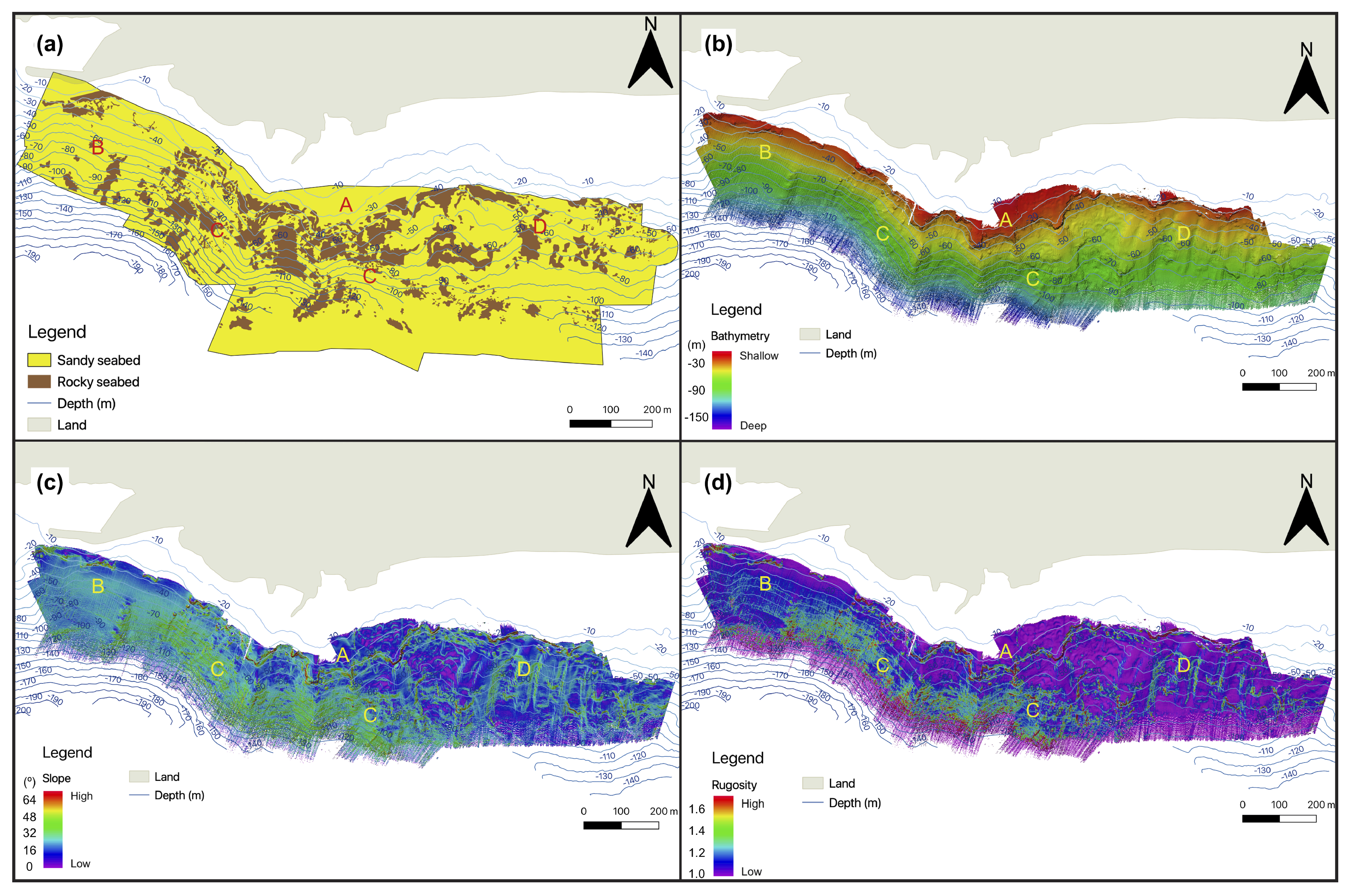
3.1. Seafloor Characteristics

3.1.1. Bathymetry and Derivative Parameters
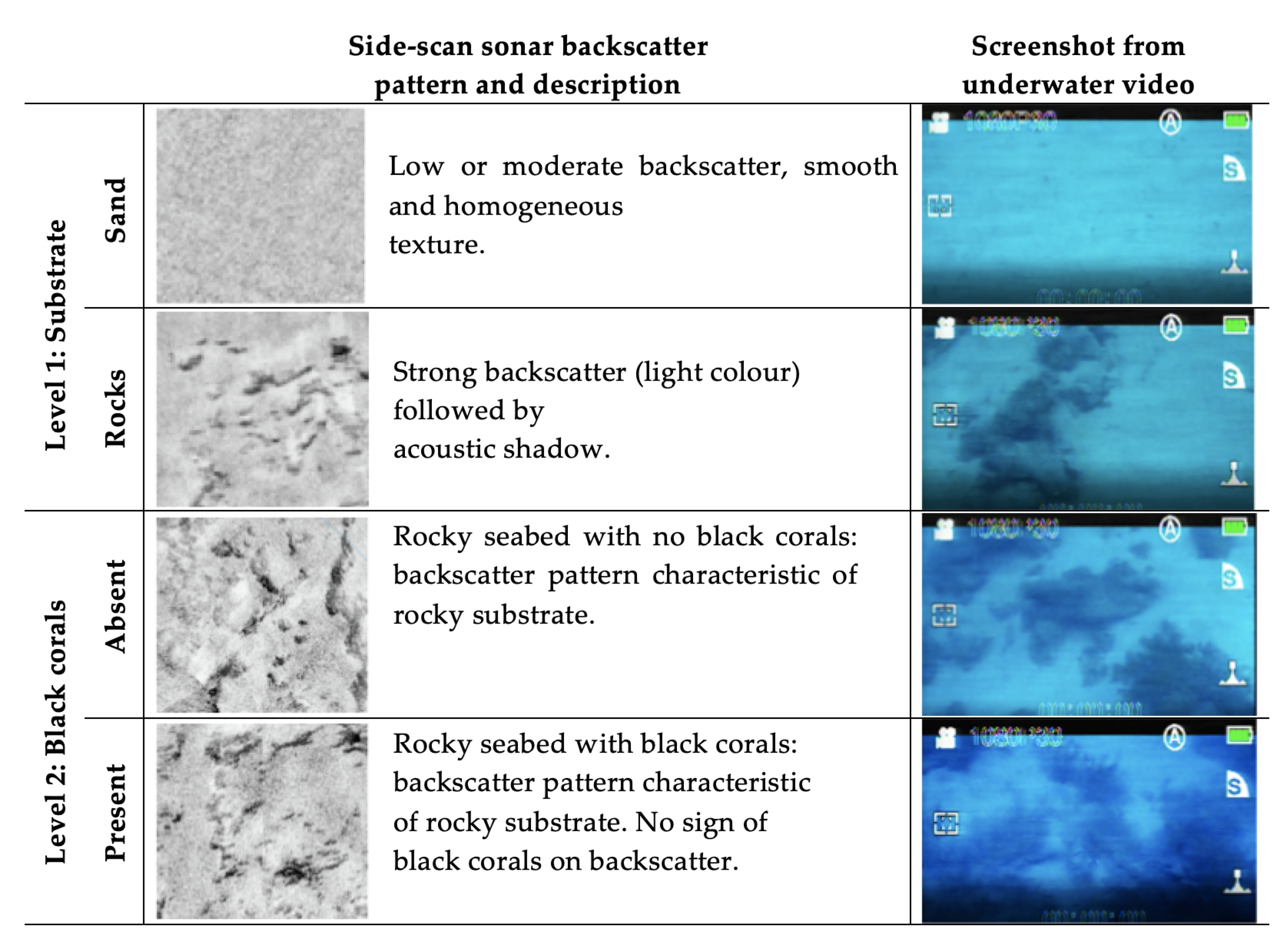
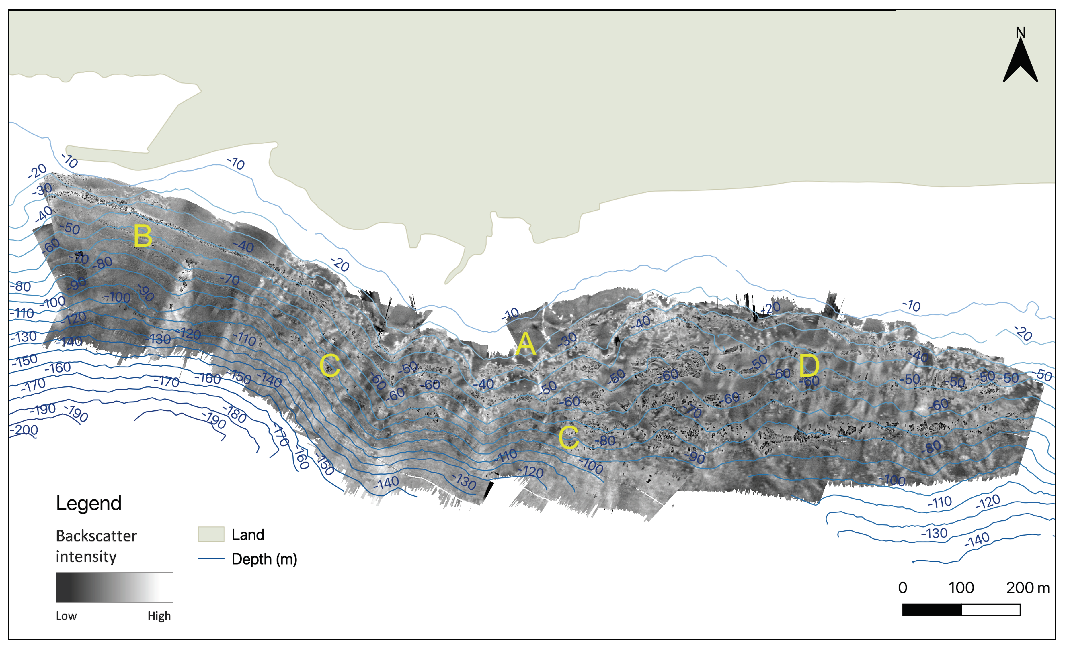
The local morphology allowed differentiating four different areas in the study site (Figure 5a). The main morphological feature was a shallow shelf down to a 36 m depth and its steep 5–15 m high drop (Zone A, Figure 5b). Here, the seafloor dropped from depths of ca. 30 m to 43 m over less than 5 m of horizontal distance in the shelf edges. The western zone (Zone B) was characterized by a smooth increase in water depth, with the exception of the NNE-SSW-directed ridge at water depths of 58 m to 118 m. In the central zone (C), below the slope A, the seafloor appeared rugged, with a number of individual mounds of circular to elliptical shapes present at the seafloor. The circumference of these features was between 6 m and 60 m. Towards the eastern zone (D), a number of almost N-S-directed channels were recorded. In some places, the depth differences between the ridges and the troughs reached 15 m. The ridge surfaces appeared smooth, while individual morphological elements were recognized in the channels.
The steepest slopes were observed in Zone A (Figure 5c), especially visible in the central part of the study area and above Part D. In these places, there were cliffs with downslope total surface distances reaching 20 m. These cliffs constitute the steepest features in the study area (i.e., slopes above 60 ). Slopes within Zone C ranged mostly between 40 and 55 . The mounds in this zone oscillated in slope between 40 and 50 , but few bigger seafloor features, such as the east-facing side of the most western trough in zone C, reached inclinations higher than 60°. Part B, apart from the NNE-SSW-directed ridge with slopes reaching above 50 , had very smooth and uniform slopes of mostly 20 to 30 . Slope values for Zone D varied, with gradually sloping platforms expanding over 200 m along the coast, as well as numerous steeper areas. Most of the steep slopes are related to the aforementioned ridge and trough system in Zone D. The steepest slopes in this zone, with inclinations above 60 , were located at the troughs ends, between 67 m and 76 m.
Generally, the rugosity index (Figure 5d) appears related to the slope, as steeper areas were commonly rougher. The shallow shelf of Zone A was smooth, which coincided with sandy bottoms in the area, whereas the shelf edges showed the highest values of rugosity. Zone B was characterized mostly by low rugosity. Zone C could be divided into two areas of different rugosity: Directly below the cliff of Zone A, the seafloor was mostly smooth, with the largest continuous areas of smooth sea bottom extending there down to 72 m depth. Below, the seafloor exhibited intermediate to high rugosity. The rugosity of Zone D followed the slope pattern, with a rougher seafloor at the sites with steeper slopes. The ridges and the floors of the trenches between them had a low rugosity. The big platforms with gentle slopes generally also showed a smooth surface.

3.1.2. Backscatter

Both the MBES (Figure 6) and SSS (Figure 4) backscatter did not provide direct visual clues about black coral occurrence when comparing locations in the backscatter mosaics with ground-truthing data. According to the SSS backscatter signatures (Figure 4), two main seafloor types were differentiated for the purpose of this study. Areas of low backscatter intensity, interpreted as sand, covered 80.5% of the surveyed seabed and corresponded to 44.2 ha. High backscatter intensity, accompanied by acoustic shadows, was interpreted as rocks and covered 19.5% of the area, corresponding to 10.7 ha.
The backscatter mosaic map (Figure 6), as well as the backscatter intensity values used for further statistical analysis (Figure 7g) were created from the MBES data. On a large scale, the backscatter of the western zone (B) was generally low; the middle zone was high (C); and the eastern zone (D) showed varied intensities. In general, the brightest areas (strongest backscatter signal) occurred in zones with the highest rugosity. Zone A was the closest to the shore and revealed a shallow shelf covered by sandy substrates, which ended with cliffs, characterized in the SSS mosaics by exposed rocks and high rugosity in the bathymetric data. Zone B constituted the western section of the studied site and was the second most sandy area after Zone A, with the exception of rocks on the most eastern side of the surveyed area, from a 10 to a 40 m depth, and a few patches in the deeper waters, including one large NNE-SSW-oriented group of boulders. Zone C was the rockiest area, with substrates generally becoming sandier below an 80 m depth. Zone D was the most heterogeneous part, with many sandy areas and patches of rocks.

3.2. Underwater Video and Diving

Underwater video and diving demonstrated differences in coral density and height with depth. Generally, the corals increased their heights with depth, also becoming denser. The results for the five transects in each area are reported in Table 1.

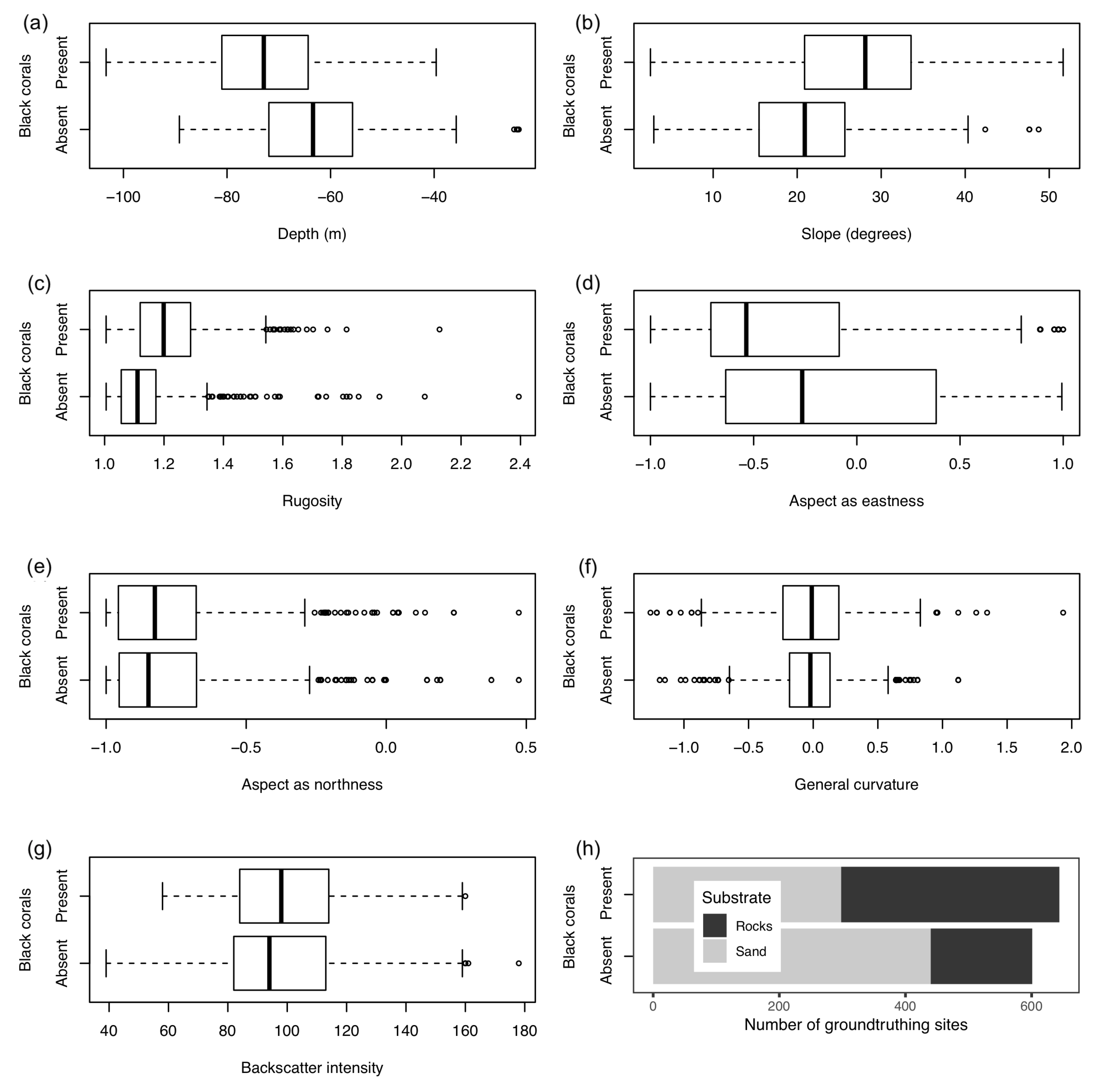
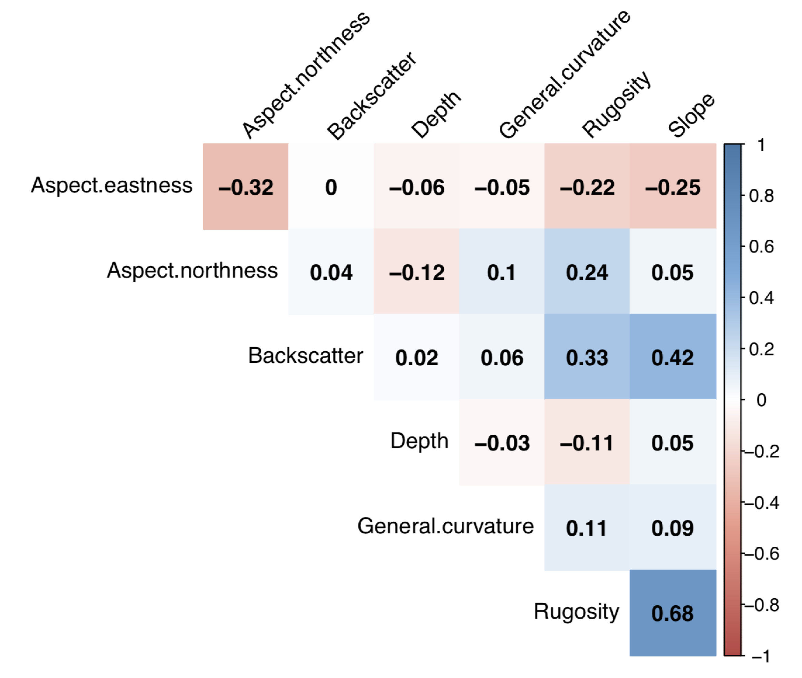
3.3. Statistical Analysis

Univariate GLMs showed that depth, slope, substrate, rugosity, and aspect eastness were, in order of decreasing importance, the strongest predictors of black coral presence, while backscatter, general curvature, and aspect northness were not significant (Figure 7 and Table A1). As Figure 7 shows, black corals were recorded in the ground-truthing videos between 40 m and over 103 m, with a major preference at larger depths (z = −12.57, p < 2 × 10⁻¹⁶; Figure 7a). The presence of corals was detected across a wide range of slopes, from almost flat (2.5 ) to very steep (51.7 ) zones. However, there were more black coral occurrences on steeper slopes, with a median value of 28.1 (z = 11.35, p < 2 × 10⁻¹⁶; Figure 7b). The rugosity index of areas both with and without black corals varied between 1.01 (not rugose, smooth terrain) and as high as 2.39 (very rough, complex terrain); antipatharian habitats were generally more rugose (z = 8.130, p < 4.30 × 10⁻¹⁶; Figure 7c). Moreover, there were significantly more black corals on westward-facing slopes (z = −7.43, p = 1.07 × 10⁻¹³; Figure 7d). Most ground-truthing locations were on southward-facing slopes, despite there being no significant effects (z = 1.12, p = 0.262; Figure 7e). The general curvature index agreed with the visual interpretations of the studied area terrain features, indicating a heterogeneous morphology with some peaks (positive values) and valleys (negative values) (z = 1.21, p = 0.228; Figure 7f). However, as most ground-truthing was done in the plain areas, both black coral presence and absence records were mostly in the plain terrain areas. In agreement with the visual interpretation of the MBES backscatter mosaic, the backscatter intensity was not correlated with black corals presence, and the backscatter strength at ground-truth sites with and without antipatharians oscillated between values of 39 and 178 (z = 1.31, p = 0.190; Figure 7g). Finally, black corals were found significantly more (z = −9.51, p < 2 × 10⁻¹⁶; Figure 7h) on substrates classified as rocks (346 records) than substrates classified as sand (298 records).
The best-fitted model with uncorrelated predictor variables (Figure A1) showed that depth, slope, aspect eastness, and substrate type affected black coral occurrence (Table 2). The presence of black corals increased with depth (estimated: −0.08, p = 3.12 × 10⁻⁸, Table 2), slope (estimated: 0.08, p = 2.26 × 10⁻¹⁰, Table 2), and aspect eastness (estimated: −0.80, p = 3.25 × 10⁻⁶, Table 2). Meanwhile, a lower presence of black corals was observed on sandy relative to rocky substrates (estimated = −0.53, p = 5.66 × 10⁻⁶, Table 2). Similar results were observed when we restricted the analysis to the deeper data subset (45 to 70 m), although black corals’ presence was mostly predicted by the slope and aspect (Table A1).

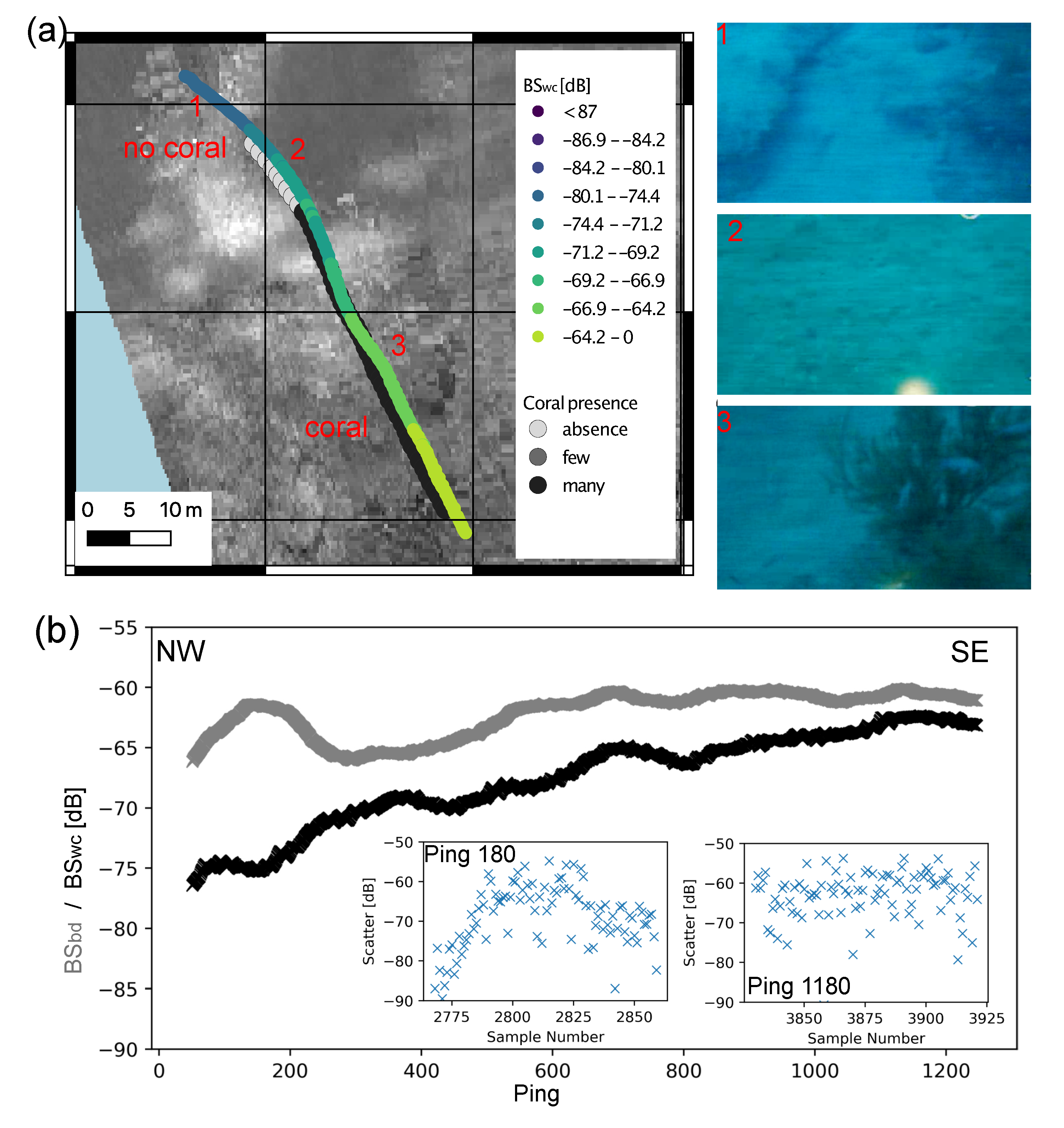
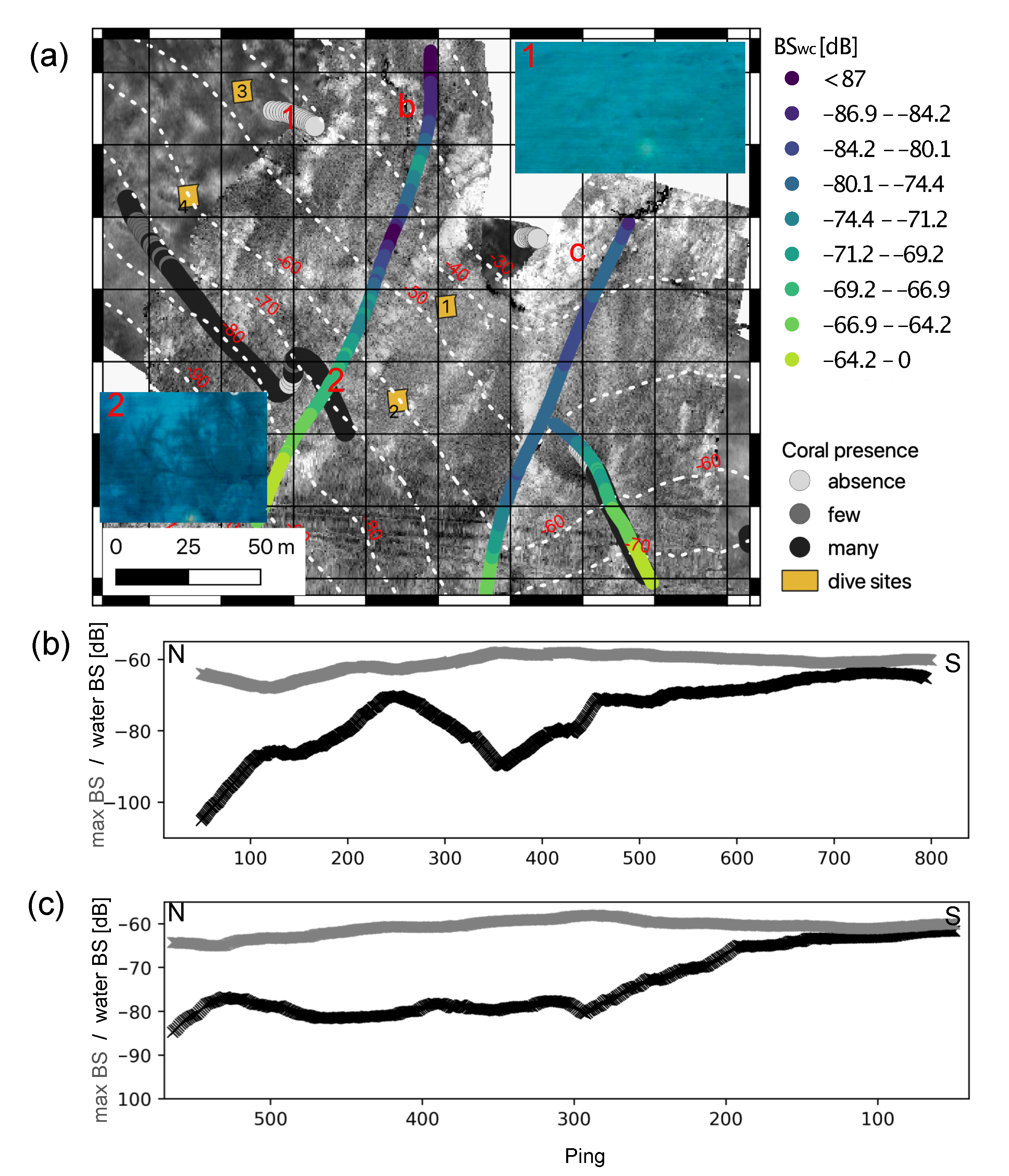
3.4. Water Column Data

As direct imaging of the corals was not possible and the correlation of backscatter intensities with coral occurrence was poor, we attempted to recognize the presence of black corals by scatter intensities in the water column data. Based on the average coral height (Table 1), the acoustic energy 75 cm to 100 cm above the bottom was considered and compared with the backscatter energy in 25 cm intervals centered on the bottom detection point.
A line recorded parallel with video ground-truthing (Figure 8) shows the transition from absent to sparse corals to coral with increasing densities towards deeper water depth. While corals are absent, the difference in scatter B S b d and B S w c is about 15 to 20 dB. Towards increasing abundance and deeper waters, a decreasing difference in scatter intensities of the water column and bottom detection samples is noted, which is clearly observed in the accompanying scatter plots of two snippets from the beginning and the end of the profile. The presence of rocks and boulders at the beginning of the profile does not reduce the distance between B S b d and B S w c . The correlation between B S b d and B S w c is 0.44 for this line, while B S w c and depth correlate with −0.74.
Two additional lines were recorded downslope from water depths of less than 20 m to a depth of 100 m (Figure 9). The beginning of the first line (Figure 9b) shows a clear differentiation between B S b d and B S w c , with differences exceeding 15 to 20 dB, in the shallow waters of seafloor Zone A, which are of predominately a sandy seafloor above the minimum depth of black corals’ occurrence. Around Ping 200, a first increase of B S w c is related to the transition of seafloor Zones A to C and a corresponding steep slope at around a 30 m depth. A strong increase B S w c occurs around Ping 450, situated at a depth of approximately 50 m slightly below the shallow diving sites. Towards deeper waters, the difference between B S b d and B S w c diminishes quickly. The correlation between B S b d and B S w c is 0.16, while the correlation between B S w c and depth is −0.64. For the second downslope line (Figure 9c) located further towards the east, the corresponding increase in values only occurs at greater depths of around 60 m. For this line, it can be observed that B S w c is not affected by the seafloor of changing backscatter composition or changes in depth from around 25 m to 50 m. Correspondingly, the correlation between B S b d and B S w c is −0.05, while the correlation between depth and B S w c remains at −0.73.

4. Discussion

4.1. Detection of Black Corals in Acoustic Data

This study tested the effectiveness of acoustic methodologies to map and characterize the habitat of A. wollastoni. Both the MBES and SSS differentiated seabed sediment types (Figure 4 and Figure 5), but did not directly reveal the presence of black corals. The arborescent structure of A. wollastoni includes a canopy of thin and complex (i.e., cm scale) branches that form a large surface (Figure 1). The individual branches are comparable to or slightly larger than the utilized acoustic wavelength of 0.003 to 0.005 m and located in the transitional zone between the Rayleigh and geometric scatter regime [65]. Therefore, a noticeable acoustic response of the branches would be expected [66], denoting the detection of black corals. Prior to the survey, it was expected that A. wollastoni would be directly recognizable on side-scan sonar backscatter mosaics. The absence of a visual signature of the black corals may be explained by the interference of rocky substrates that mask the black coral acoustic pattern [67]. The high elevation of the towfish above the seafloor (to avoid contact with the seafloor in this challenging environment) may have contributed to the loss of the signatures of individual corals. Still, this does not convincingly explain why coral patches situated on sandy seabeds were not reliably differentiated from the surrounding seafloor by the towed side-scan sonar towfish (Figure 4). A possibility is that the side-scan sonar frequency of 325 kHz interacts unfavorably with the black coral branches, especially given their proteinaceous skeletons [24], limiting their detectability. Further studies using dual-frequency SSS located closer to the sea bottom to decrease acoustic footprints and increase mosaic resolution are recommended.
In contrast to side-scan sonar data, the MBES-derived data were not expected to identify individual coral patches due to the extended footprint size in 40 m water depths and greater. However, the system provided ample morphological and derived information about the habitats where black corals occur (Figure 5). Slope and rugosity data were correlated, which is expected because steeper areas tend to be rougher, due to a lack of sediment accumulation and, consequently, the exposure of the volcanic substratum [68]. The statistical analysis revealed the relationship between antipatharian presence and the data (i.e. habitat features) produced by the MBES. Our statistical model showed increased presence of black corals at greater depths and in areas with rocky substrate, steep slopes, and high rugosity. Based on bathymetric data, the best option to detect black corals could be the observed relationship between black coral occurrence and their impact on seafloor topography, here expressed by rugosity (Figure 7). In this study, rugosity was calculated using a 3 × 3 kernel operating on the bathymetric grid. The resolution of the rugosity analysis could be much improved by operating directly on the pre-grid point cloud data of the multibeam echo sounder [69], a method that was recently suggested by [70] for the detection of seagrass.
An additional advantage of modern multibeam echo sounder data is the collection of backscatter information around the bottom detection point (snippets), which can be used for seafloor classification [71,72]. As displayed in Figure 8 and Figure 9, based on the available ground-truthing, the water column backscatter B S w c is sensitive to the occurrence of black corals, with the coral skeletons increasing scatter in the water column. Comparable approaches were recently utilized to detect giant kelp forests in MBES-derived water column data [73]. The water column scatter at 0.75 m to 1.0 m above the seafloor is in principle not affected by the geological seafloor composition (rock/sand), as clearly demonstrated by the low correlation between the water column signal and the backscatter around the bottom detection point.
However, misclassification occurs in areas of steep slope, when the footprint of the system encompasses a significant morphology. For vertical incidence in a long-pulse regime [66], footprint sizes of the NORBITiwbmse system used (0.9 × 1.9 resolution) changed from 0.16 m 2 (20 m water depth) to 0.65 m 2 (40 m water depth) to 2.6 m 2 (80 m water depth). In the long-pulse regime, the entire footprint is insonifed simultaneously, and steep local morphologies can appear as increasing water column scatter in the snippet time series. Especially in rough and steep environments, these effects can be expected to become more significant with depth. It is furthermore difficult to disentangle the correlation of B S w c with depth and coral occurrence, as the black corals also are increasingly abundant and larger with depth (Figure 7, Table 1). However, the partial decrease of water column scatter with depth (Figure 9, Profile B) and the different increases of water column scatter with depth for the two downslope profiles (Figure 9, Profiles B and C)—in line with nearby ground-truthing stations—are promising indications that B S w c is at least partially impacted by black coral skeletons and can be used to map their presence.
An additional limitation of this study is the recorded snippet range of 1 m above and below the bottom detection point. Since black coral colonies are frequently larger, especially in deep waters, the onset of corals is missed and more advanced snippet characterization [71] not meaningful. The problem becomes worse for oblique beams, which are also increasingly affected by natural changes of morphology within their footprint. Therefore, it is suggested for future surveys to record water column scatter up to 2 m above the bottom detection point for all incidence angles.

4.2. Implications for Black Coral Habitats Offshore Lanzarote

Despite being unable to produce A. wollastoni distribution maps, the acoustic tools provided information about seabed morphology and structure, which allowed constraining the A. wollastoni habitat offshore Lanzarote. A number of studies have used the digital terrain data obtained from the MBES bathymetry to improve local scale (i.e., 10 to 100 km 2 ) models of species distributions [61,74,75,76]. The ground-truthing data of this study were limited to maximum depths of ca. 100 m. Therefore, it is not possible to state what is the optimum range and maximum depth for A. wollastoni. However, the data showed that the upper depth limit for this species off the Lanzarote coast is ca. 40 m, which is supported by previous studies in the Canary Islands [50,51]. The antipatharians showed a preference for rocks as the substrate, which confirms that many black coral species require a hard substrate for attachment [77,78]. The fact that some black corals were recorded on sandy bottoms may be because the sites were actually hiding rocks beneath a layer of sand. The penetration of the high frequency acoustic waves used (>300 kHz) into sand is less than a few cm; therefore, underlying rocks are not captured by the acoustic methods. Increased sediment retention is one of the characteristics of gorgonian coral gardens [79], and it is likely that the antipatharian aggregations studied do the same. Here, using additional low frequencies for mapping—found to be advantageous for habitat mapping in several instances [80,81]—could provide additional information about areas covered by a few centimeters of sand only.
Increased occurrence on rocks, as well as on large slopes and rugged grounds, may hint at A. wollastoni’s preference for specific terrain features, such as cracks and depressions on steep ledges; similar patterns have been observed for Hawaiian black corals (Antipathes spp.; [82]). It is also possible that the species’ preferred features are topographic forms that may experience increased hydrodynamic energy [83], promoting antipatharian performance, as strong currents provide more food for these filter-feeding animals [24]. This explanation stays in agreement with observations by [84], where strong currents are a common feature in A. wollastoni-dominated habitats in the Canary Islands. In this regard, an interesting finding in this study was the importance of the slope, with the black corals found more often on the more west-facing slopes. This may be due to stronger local currents operating on the west-facing slopes. However, current information on such a small scale is not available, and the underlying causes of this finding need further investigation.

5. Conclusions

Black corals gardens were not directly mapped in backscatter mosaics and bathymetric maps recorded by the multibeam echo sounder or side-scan sonar. The use of water column scatter measured by multibeam echo sounder data to detect coral skeletons above the seafloor appears promising and should be further explored in future studies to obtain full-coverage spatial maps. Additionally, a correlation between the occurrence of A. wollastoni and seafloor rugosity was found, which could be further exploited in the future by utilizing point-based classification techniques on MBES data combined with high-resolution photogrammetric techniques. Offshore Lanzarote, A. wollastoni gardens occur with increasing abundance at depths below 40 m, particularly at steep slopes with rocky substrates and complex topography. Colonies of A. wollastoni occurred more often on westward slopes, which may be related to local oceanographic conditions.

Author Contributions

Conceptualization P.F. and F.O.-F.; validation, data curation, visualization, and funding acquisition K.C., P.F., and F.O.-F.; project administration F.O.-F.; methodology K.C., P.F., M.C.d.E., and F.O.-F.; software and formal analysis K.C., P.F., F.T., M.C.d.E., M.S., and F.O.-F.; investigation K.C., P.F., F.E., and F.O.-F.; resources P.F., F.O.-F., and R.H.; writing, original draft preparation K.C.; writing, review and editing K.C., P.F., F.T., F.E., M.C., M.S., R.H., and F.O.-F.; supervision P.F., R.H., and F.O.-F. All authors read and agreed to the published version of the manuscript.

Funding

This research was partially financed by Universidad de Las Palmas de Gran Canaria (ULPGC), Leibniz Institute for Baltic Sea Research Warnemünde (IOW), the Clear Reef Social Fund for Marine Research and Conservation (Session 2019) and LIFE Programme of the European Union, the French Office for Biodiversity (OFB) and the French Development Agency (AFD) through the LIFE4BEST Programme. The contents of this document are the sole responsibility of B-CHARMED project (LIFE4BEST GA-2019-M-9) and can under no circumstances be regarded as reflecting the position of the European Union nor of the OFB and AFD. The publication of this article was funded by the Open Access Fund of the Leibniz Association.

Acknowledgments

We gratefully thank Andreas Frahm and Acisclo Jose Concepcion Lorenzo for their extraordinary support during the fieldwork. Moreover, we acknowledge Alejandro García Mendoza for GIS assistance.

Conflicts of Interest

The authors declare no conflict of interest. The funders had no role in the design of the study; in the collection, analyses, or interpretation of data; in the writing of the manuscript; nor in the decision to publish the results.

Appendix A

Table A1. Results of the GLM, using a binomial family distribution of errors and a logit link function, to assess the effect of habitat predictors on the presence of black corals.
Factorz-Valuep-ValueReduction in Deviance
full dataset: all depths (25 m–100 m)
Depth−12.570<2 × 10−16202.40
Slope11.350<2 × 10−16149.60
Rugosity8.1304.3 × 10−1680.50
Aspect eastness−7.4321.07 × 10−1358.30
Aspect northness1.1220.2621.30
General curvature1.2070.2281.50
Backscatter1.3100.1901.80
Substrate: sand−8.231<2 × 10−1698.00
Data subset: 45 m–70 m depth
Depth−5.0055.58 × 10−726.71
Slope7.3122.64 × 10−1362.27
Rugosity3.6322.81 × 10−414.44
Aspect eastness−5.8983.68 × 10−937.46
Aspect northness1.5390.1242.38
General curvature1.7470.0813.08
Backscatter−0.3650.7150.13
Substrate: sand−2.4860.01314.41
Figure A1. Correlation matrix for the MBES-derived variables for a data subset containing the 45 m–70 m ground-truth. The numbers are Pearson correlation coefficients, with color intensity proportional to the strength of the correlation: blue—negative correlation; red—positive correlation.
Remotesensing 12 03244 g0a1

References

  1. EC. Directive of the European Parliament and the Council Establishing a Framework for Community Action in the Field of Marine Environmental Policy (Marine Strategy Framework Directive); Directive 2008/56/ EC, OJ L 164; European Commission: Brussels, Belgium, 2008. [Google Scholar]
  2. EEC. Habitats Directive 92/43/EEC; OJ L 206; European Commission: Brussels, Belgium, 1992. [Google Scholar]
  3. UN. Convention on Biological Diversity; art. 1, 31 I.L.M. 818; United Nations: Rio de Janeiro, Brazil, 1992. [Google Scholar]
  4. Buhl-Mortensen, L.; Buhl-Mortensen, P.; Dolan, M.; Gonzalez-Mirelis, G. Habitat mapping as a tool for conservation and sustainable use of marine resources: Some perspectives from the MAREANO Programme, Norway. J. Sea Res. 2015, 100, 46–61. [Google Scholar] [CrossRef]
  5. Harris, P.; Baker, E. (Eds.) Seafloor Geomorphology As Benthic Habitat. GeoHab Atlas of Seafloor Geomorphic Features and Benthic Habitats; Elsevier: Amsterdam, The Netherlands, 2020; p. 1030. [Google Scholar]
  6. Jordan, A.; Lawler, M.; Halley, V.; Barrett, N. Seabed habitat mapping in the Kent Group of islands and its role in marine protected area planning. Aquat. Conserv. Mar. Freshw. Ecosyst. 2005, 15, 51–70. [Google Scholar] [CrossRef]
  7. Mumby, P.; Green, E.; Edwards, A.; Clark, C. The cost-effectiveness of remote sensing for tropical coastal resources assessment and management. J. Environ. Manag. 1999, 55, 157–166. [Google Scholar] [CrossRef]
  8. Sini, M.; Katsanevakis, S.; Koukourouvli, N.; Gerovasileiou, V.; Dailianis, T.; Buhl-Mortensen, L.; Damalas, D.; Dendrinos, P.; Dimas, X.; Frantzis, A. Assembling ecological pieces to reconstruct the conservation puzzle of the Aegean Sea. Front. Mar. Sci. 2017, 4, 347. [Google Scholar] [CrossRef]
  9. Brown, C.J.; Smith, S.J.; Lawton, P.; Anderson, J.T. Benthic habitat mapping: A review of progress towards improved understanding of the spatial ecology of the seafloor using acoustic techniques. Estuarine Coast. Shelf Sci. 2011, 92, 502–520. [Google Scholar] [CrossRef]
  10. Collings, S.; Campbell, N.A.; Keesing, J.K. Quantifying the discriminatory power of remote sensing technologies for benthic habitat mapping. Int. J. Remote Sens. 2019, 40, 2717–2738. [Google Scholar] [CrossRef]
  11. Gavazzi, G.M.; Madricardo, F.; Janowski, L.; Kruss, A.; Blondel, P.; Sigovini, M.; Foglini, F. Evaluation of seabed mapping methods for fine-scale classification of extremely shallow benthic habitats–application to the Venice Lagoon, Italy. Estuarine Coast. Shelf Sci. 2016, 170, 45–60. [Google Scholar] [CrossRef] [Green Version]
  12. Costa, B.; Battista, T.; Pittman, S. Comparative evaluation of airborne LiDAR and ship-based multibeam SoNAR bathymetry and intensity for mapping coral reef ecosystems. Remote Sens. Environ. 2009, 113, 1082–1100. [Google Scholar] [CrossRef]
  13. Komatsu, T.; Igararashi, C.; Tatsukawa, K.I.; Nakaoka, M.; Hiraishi, T.; Taira, A. Mapping of seagrass and seaweed beds using hydro-acoustic methods. Fish. Sci. 2002, 68, 580–583. [Google Scholar] [CrossRef] [Green Version]
  14. Cosme, M.; Otero-Ferrer, F.; Tuya, F.; Espino, F.; Abreu, A.D.; Haroun, R. Mapping Subtropical and Tropical Rhodolith Seabeds Using Side Scan Sonar Technology. In Proceedings of the 6th International Rhodolith Workshop, Roscoff, France, 25–29 June 2018. [Google Scholar]
  15. Freiwald, A. Reef-forming cold-water corals. In Ocean Margin Systems; Springer: Berlin/Heidelberg, Germany, 2002. [Google Scholar]
  16. Roberts, J.; Brown, C.; Long, D.; Bates, C. Acoustic mapping using a multibeam echosounder reveals cold-water coral reefs and surrounding habitats. Coral Reefs 2005, 24, 654–669. [Google Scholar] [CrossRef]
  17. Glogowski, S.; Dullo, W.C.; Feldens, P.; Liebetrau, V.; von Reumont, J.; Hühnerbach, V.; Krastel, S.; Wynn, R.B.; Flögel, S. The Eugen Seibold coral mounds offshore western Morocco: Oceanographic and bathymetric boundary conditions of a newly discovered cold-water coral province. Geo-Mar. Lett. 2015, 35, 257–269. [Google Scholar] [CrossRef] [Green Version]
  18. Kenny, A. An overview of seabed-mapping technologies in the context of marine habitat classification. ICES J. Mar. Sci. 2003, 60, 411–418. [Google Scholar] [CrossRef] [Green Version]
  19. Blondel, P. The Handbook of Sidescan Sonar; Springer: Berlin, Germany; New York, NY, USA; Praxis Pub: Chichester, UK, 2009; p. 316. [Google Scholar]
  20. Cobra, D.; Oppenheim, A.; Jaffe, J. Geometric distortions in side-scan sonar images: A procedure for their estimation and correction. IEEE J. Ocean. Eng. 1992, 17, 252–268. [Google Scholar] [CrossRef]
  21. Cervenka, P.; Moustier, C.D.; Lonsdale, P.F. Geometric corrections on sidescan sonar images based on bathymetry. Application with SeaMARC II and Sea Beam data. Mar. Geophys. Res. 1994, 16, 365–383. [Google Scholar] [CrossRef]
  22. Shang, X.; Zhao, J.; Zhang, H. Obtaining High-Resolution Seabed Topography and Surface Details by Co-Registration of Side-Scan Sonar and Multibeam Echo Sounder Images. Remote Sens. 2019, 11, 1496. [Google Scholar] [CrossRef] [Green Version]
  23. Fakiris, E.; Blondel, P.; Papatheodorou, G.; Christodoulou, D.; Dimas, X.; Georgiou, N.; Kordella, S.; Dimitriadis, C.; Rzhanov, Y.; Geraga, M.; et al. Multi-Frequency, Multi-Sonar Mapping of Shallow Habitats—Efficacy and Management Implications in the National Marine Park of Zakynthos, Greece. Remote Sens. 2019, 11, 461. [Google Scholar] [CrossRef] [Green Version]
  24. Wagner, D.; Luck, D.; Toonen, R. The biology and ecology of black corals (Cnidaria: Anthozoa: Hexacorallia: Antipatharia). Adv. Mar. Biol. 2012, 63, 67–132. [Google Scholar]
  25. Appeltans, W.; Ahyong, S.; Anderson, G.; Angel, M.; Artois, T.T. The Magnitude of Global Marine Species Diversity. Curr. Biol. 2012, 22, 2189–2202. [Google Scholar] [CrossRef] [Green Version]
  26. Roberts, J.; Wheeler, A.; Freiwald, A.; Cairns, S. Cold-Water Corals: The Biology and Geology of Deep-Sea Coral Habitats; Cambridge University Press: Cambridge, UK, 2009; p. 334. [Google Scholar]
  27. Brook, G. Report on the Antipatharia collected by HMS Challenger during the years 1873–1876. Chall. Rep. Zool. 1889, 32, 1–222. [Google Scholar]
  28. ICES. Report of the Working Group on Deep-Water Ecology (WGDEC); ICES Advisory Committee on Ecosystems; ICES Document CM 2007/ACE:01; ICES: Copenhagen, Denmark, 2007. [Google Scholar]
  29. De Clippele, L.; Huvenne, V.; Molodtsova, T.; Roberts, J.M. The diversity and ecological role of non-scleractinian corals (Antipatharia and Alcyonacea) on scleractinian cold-water coral mounds. Front. Mar. Sci. 2019, 6, 184. [Google Scholar] [CrossRef]
  30. Freiwald, A.; Fossa, J.; Grehan, A.; Koslow, T.; Roberts, J. Cold-Water Coral Reefs: Out of Sight-No Longer out of Mind; UNEP-WCMC: Cambridge, UK, 2004. [Google Scholar]
  31. Krieger, K.; Wing, B. Megafauna associations with deepwater corals (Primnoa spp.) in the Gulf of Alaska. Hydrobiologia 2002, 471, 83–90. [Google Scholar] [CrossRef]
  32. Tazioli, S.; Bo, M.; Boyer, M.; Rotinsulu, H.; Bavestrello, G. Ecological observations of some common antipatharian corals in the marine park of Bunaken (North Sulawesi, Indonesia). Zool. Stud. 2007, 46, 227–241. [Google Scholar]
  33. Herler, J. Microhabitats and ecomorphology of coral-and coral rock-associated gobiid fish (Teleostei: Gobiidae) in the northern Red Sea. Mar. Ecol. 2007, 28, 82–94. [Google Scholar] [CrossRef]
  34. Tissot, B.N.; Yoklavich, M.M.; Love, M.S.; York, K.; Amend, M. Benthic invertebrates that form habitat on deep banks off southern California, with special reference to deep sea coral. Fish. Bull. 2006, 104, 167–181. [Google Scholar]
  35. Angel, M.; Boxhal, G. Life in the benthic boundary layer: Connections to the mid-water and sea floor. Philos. Trans. R. Soc. Lond. Ser. A Math. Phys. Sci. 1990, 331, 15–28. [Google Scholar]
  36. Bo, M.; Tazioli, S.; Spanò, N.; Bavestrello, G. Antipathella subpinnata (Antipatharia, Myriopathidae) in Italian seas. Ital. J. Zool. 2008, 75, 185–195. [Google Scholar] [CrossRef]
  37. Humes, A.; Goenaga, C. Calonastes imparipes, new genus, new species (Copepoda, Cyclopoida), associated with the antipatharian coral genus Stichopathes in Puerto Rico. Bull. Mar. Sci. 1978, 28, 189–197. [Google Scholar]
  38. Baillon, S.; Hamel, J.; Wareham, V.; Mercier, A. Deep cold-water corals as nurseries for fish larvae. Front. Ecol. Environ. 2012, 10, 351–356. [Google Scholar] [CrossRef] [Green Version]
  39. Gomes-Pereira, J.; Carmo, V.; Catarino, D.; Jakobsen, J.; Alvarez, H.; Aguilar, R.; Hart, J.; Giacomello, E.; Menezes, G.; Stefanni, S.; et al. Cold-water corals and large hydrozoans provide essential fish habitat for Lappanella fasciata and Benthocometes robustus. Deep Sea Res. Part II Trop. Stud. Oceanogr. 2017, 145, 33–48. [Google Scholar] [CrossRef]
  40. Molodtsova, T.; Budaeva, N. Modifications of corallum morphology in black corals as an effect of associated fauna. Bull. Mar. Sci. 2007, 81, 469–479. [Google Scholar]
  41. Andrews, A.; Stone, R.; Lundstrom, C.; DeVogelaere, A. Growth rate and age determination of bamboo corals from the northeastern Pacific Ocean using refined 210 Pb dating. Mar. Ecol. Prog. Ser. 2009, 397, 173–185. [Google Scholar] [CrossRef]
  42. Roark, E.; Guilderson, T.; Dunbar, R.; Fallon, S.; Mucciarone, D. Extreme longevity in proteinaceous deep-sea corals. Proc. Natl. Acad. Sci. USA 2009, 106, 5204–5208. [Google Scholar] [CrossRef] [PubMed] [Green Version]
  43. Wagner, D.; Opresko, D. Description of a new species of Leiopathes (Antipatharia: Leiopathidae) from the Hawaiian Islands. Zootaxa 2015, 3974, 277–289. [Google Scholar] [CrossRef] [Green Version]
  44. Clark, M.; Rowden, A. Effect of deepwater trawling on the macro-invertebrate assemblages of seamounts on the Chatham Rise, New Zealand. Deep Sea Res. Part I Oceanogr. Res. Pap. 2009, 56, 1540–1554. [Google Scholar] [CrossRef]
  45. Todinanahary, G.; Terrana, L.; Lavitra, T.; Eeckhaut, I. First records of illegal harvesting and trading of black corals (Antipatharia) in Madagascar. Madag. Conserv. Dev. 2016, 11. [Google Scholar] [CrossRef] [Green Version]
  46. Rogers, A.; Gianni, M. The Implementation of UNGA Resolutions 61/105 and 64/72 in the Management of Deep-Sea Fisheries on the High Seas—A Report from the International Programme on the State of the Ocean; Report Prepared for the Deep-Sea Conservation Coalition; International Programme on the State of the Ocean: London, UK, 2011; 97p. [Google Scholar]
  47. Fuller, S.; Murillo, F.; Wareham, V.; Kenchington, E. Vulnerable Marine Ecosystems Dominated by Deep-Water Corals and Sponges in the NAFO Convention Area; Serial No N5524; NAFO: Dartmouth, NS, Canada, 2008. [Google Scholar]
  48. De Matos, V.; Gomes-Pereira, J.N.; Tempera, F.; Ribeiro, P.A.; Braga-Henriques, A.; Porteiro, F. First record of Antipathella subpinnata (Anthozoa, Antipatharia) in the Azores (NE Atlantic), with description of the first monotypic garden for this species. Deep Sea Res. Part II Top. Stud. Oceanogr. 2014, 99, 113–121. [Google Scholar] [CrossRef]
  49. Gray, D. Synopsis of the families and genera of axiferous zoophytes or barked corals. Proc. Zool. Soc. Lond. 1857, 25, 278–294. [Google Scholar] [CrossRef]
  50. Bianchi, C.; Haroun, R.; Morri, C.; Wirtz, P. The subtidal epibenthic communities off Puerto del Carmen (Lanzarote, Canary Islands). Arquipélago 2000, 2, 145–155. [Google Scholar]
  51. Martín-García, L.; Brito-Izquierdo, I.; Brito-Hernández, A. Changes in benthic communities due to submarine volcanic eruption: Black coral (Antipathella wollastoni) death in the Marine Reserve of El Hierro (Canary Islands). Rev. Acad. Canar. Cienc. 2015, 27, 345–353. [Google Scholar]
  52. Domínguez, L.; Ferrer, F. Aquaculture and marine biodiversity boost: Case examples from the Canary Islands. Water Resour. Manag. 2009, 97, 97–102. [Google Scholar]
  53. Riera, R.; Becerro, M.; Stuart-Smith, R.; Delgado, J.; Edgar, G. Out of sight, out of mind: Threats to the marine biodiversity of the Canary Islands (NE Atlantic Ocean). Mar. Pollut. Bull. 2014, 86, 9–18. [Google Scholar] [CrossRef]
  54. Martín-García, L.; Brito-Izquierdo, I.; Brito-Hernández, A. Bionomía bentónica de las Reservas Marinas de Canarias (España). Comunidades y hábitats bentónicos del infralitoral; Ministerio de Agricultura y Pesca, Alimentación y Medio Ambiente: Madrid, Spain, 2016; p. 181. [Google Scholar]
  55. Acosta, J.; Uchupi, E.; Muñoz, A.; Herranz, P.; Palomo, C.; Ballesteros, M.; Group, Z.W. Geologic evolution of the Canarian Islands of Lanzarote, Fuerteventura, Gran Canaria and La Gomera and comparison of landslides at these islands with those at Tenerife, La Palma and El Hierro. Mar. Geophys. Res. 2003, 24, 1–40. [Google Scholar] [CrossRef]
  56. Van den Bogaard, P. The origin of the Canary Island Seamount Province-New ages of old seamounts. Sci. Rep. 2013, 3, 2107. [Google Scholar] [CrossRef] [Green Version]
  57. Mann, K.; Lazier, J. Dynamics of Marine Ecosystems: Biological-Physical Interactions in the Oceans; Blackwell Scientific Publiations: Boston, MA, USA, 2013; p. 446. [Google Scholar]
  58. Guinotte, J.; Davies, A. Predicted Deep-Sea Coral Habitat Suitability for Alaskan Waters; Report to NOAA-NMFS; NOAA-NMFS: Seattle, WA, USA, 2013; p. 22. [Google Scholar]
  59. Yesson, C.; Bedford, F.; Rogers, A.; Taylor, M. The global distribution of deep-water Antipatharia habitat. Deep Sea Res. Part II Top. Stud. Oceanogr. 2017, 145, 79–86. [Google Scholar] [CrossRef]
  60. Schnyder, J.; Eberli, G.; Kirby, J.; Shi, F.; Tehranirad, B.; Mulder, T.; Ducassou, E.; Hebbeln, D.; Wintersteller, P. Tsunamis caused by submarine slope failures along western Great Bahama Bank. Sci. Rep. 2016, 6, 35925. [Google Scholar] [CrossRef] [PubMed] [Green Version]
  61. Wilson, M.; O’Connell, B.; Brown, C.; Guinan, J.; Grehan, A. Multiscale terrain analysis of multibeam bathymetry data for habitat mapping on the continental slope. Mar. Geod. 2007, 30, 3–35. [Google Scholar] [CrossRef] [Green Version]
  62. Zevenbergen, L.; Thorne, C. Quantitative analysis of land surface topography. Earth Surf. Process. Landf. 1987, 12, 47–56. [Google Scholar] [CrossRef]
  63. R Core Team. A Language and Environment for Statistical Computing; R Foundation for Statistical Computing: Vienna, Austria, 2016. [Google Scholar]
  64. Wei, T.; Simko, V. R Package “Corrplot”: Visualization of a Correlation Matrix, Version 0.84; CRAN: Wien, Austria, 2017. [Google Scholar]
  65. Buscombe, D.; Grams, P.E.; Kaplinski, M.A. Compositional Signatures in Acoustic Backscatter Over Vegetated and Unvegetated Mixed Sand-Gravel Riverbeds. J. Geophys. Res. Earth Surf. 2017, 122, 1771–1793. [Google Scholar] [CrossRef] [Green Version]
  66. Lurton, X.; Lamarche, G.; Brown, C.; Lucieer, V.; Rice, G.; Schimel, A.; Weber, T. Backscatter Measurements by Seafloor-Mapping Sonars Guidelines and Recommendations. 2015, p. 200. Available online: https://www.semanticscholar.org/paper/Backscatter-measurements-by-seafloor%E2%80%90mapping-and-Lurton-Lamarche/792763b9321fe1c0408fc260e8a3e57fd3d0192f (accessed on 11 September 2020).
  67. Simmonds, J. Survey design for acoustic seabed classification. In Acoustic Seabed Classification of Marine Physical and Biological Landscapes; Anderson, J., Ed.; International Council for the Exploration of the Sea: Copenhagen, Danmark, 2007; pp. 132–138. [Google Scholar]
  68. Lurton, X. An Introduction to Underwater Acoustics: Principles and Applications; Springer Science & Business Media: Berlin, Germany, 2002. [Google Scholar]
  69. Buscombe, D. Spatially explicit spectral analysis of point clouds and geospatial data. Comput. Geosci. 2016, 86, 92–108. [Google Scholar] [CrossRef] [Green Version]
  70. Held, P.; von Schneider Deimling, J. New Feature Classes for Acoustic Habitat Mapping—A Multibeam Echosounder Point Cloud Analysis for Mapping Submerged Aquatic Vegetation (SAV). Geosciences 2019, 9, 235. [Google Scholar] [CrossRef] [Green Version]
  71. Janowski, L.; Tęgowski, J.; Nowak, J. Seafloor mapping based on multibeam echosounder bathymetry and backscatter data using Object-Based Image Analysis: A case study from the Rewal site, the Southern Baltic. Oceanol. Hydrobiol. Stud. 2018, 47, 248–259. [Google Scholar] [CrossRef]
  72. Tęgowski, J. Acoustical classification of the bottom sediments in the southern Baltic Sea. Quat. Int. 2005, 130, 153–161. [Google Scholar] [CrossRef]
  73. Schimel, A.C.G.; Brown, C.J.; Ierodiaconou, D. Automated Filtering of Multibeam Water-Column Data to Detect Relative Abundance of Giant Kelp (Macrocystis pyrifera). Remote Sens. 2020, 12, 1371. [Google Scholar] [CrossRef]
  74. Holmes, K.; Niel, K.V.; Radford, B.; Kendrick, G.; Grove, S. Modelling distribution of marine benthos from hydroacoustics and underwater video. Cont. Shelf Res. 2008, 28, 1800–1810. [Google Scholar] [CrossRef]
  75. Guinan, J.; Brown, C.; Dolan, M.; Grehan, A. Ecological niche modeling of the distribution of cold-water coral habitat using underwater remote sensing data. Ecol. Inform. 2009, 4, 83–92. [Google Scholar] [CrossRef]
  76. Rengstorf, A.; Grehan, A.; Yesson, C.; Brown, C. Towards high-resolution habitat suitability modeling of vulnerable marine ecosystems in the deep-sea: Resolving terrain attribute dependencies. Mar. Geod. 2012, 35, 343–361. [Google Scholar] [CrossRef]
  77. Grigg, R.; Opresko, D. Order Antipatharia, black corals. In Reef and Shore Fauna of Hawaii. Section 1: Protozoa through Ctenophora; Devaney, D., Eldredge, L., Eds.; Bishop Museum Press: Honolulu, HI, USA, 1977; pp. 242–261. [Google Scholar]
  78. Opresko, D.M. Review of the genus Schizopathes (Cnidaria: Antipatharia: Schizopathidae) with a description of a new species from the Indian Ocean. Oceanogr. Lit. Rev. 1998, 1, 115. [Google Scholar]
  79. Cerrano, C.; Danovaro, R.; Gambi, C.; Pusceddu, A.; Riva, A.; Schiaparelli, S. Gold coral (Savalia savaglia) and gorgonian forests enhance benthic biodiversity and ecosystem functioning in the mesophotic zone. Biodivers. Conserv. 2010, 19, 153–167. [Google Scholar] [CrossRef] [Green Version]
  80. Brown, C.J.; Beaudoin, J.; Brissette, M.; Gazzola, V. Multispectral Multibeam Echo Sounder Backscatter as a Tool for Improved Seafloor Characterization. Geosciences 2019, 9, 126. [Google Scholar] [CrossRef] [Green Version]
  81. Feldens, P.; Schulze, I.; Papenmeier, S.; Schönke, M.; Schneider von Deimling, J. Improved Interpretation of Marine Sedimentary Environments Using Multi-Frequency Multibeam Backscatter Data. Geosciences 2018, 8, 214. [Google Scholar] [CrossRef]
  82. Grigg, R. Ecological studies of black coral in Hawaii. Pac. Sci. 1965, 19, 244–260. [Google Scholar]
  83. Talley, L. Descriptive Physical Oceanography: An Introduction; Elsevier: Amsterdam, The Netherlands, 2011; p. 564. [Google Scholar]
  84. Brito, A.; Ocaña, B. Corales de las Islas Canarias: Antozoos con Esqueleto de los Fondos Litorales y Profundos; Francisco Lemus: La Laguna, Spain, 2004; p. 477. [Google Scholar]
Figure 1. Antipathella wollastoni garden off the Lanzarote coast (Canary Islands, Spain). Photo credit: Aquacine© (www.aquacine.net).
Remotesensing 12 03244 g001
Figure 2. Study area off Lanzarote Island (Canary Islands, eastern Atlantic Ocean) (red arrow). Polygons represent acoustic surveys’ coverage: yellow—side-scan sonar (SSS); grey—multibeam echosounder (MBES); black points denote ground-truthing underwater camera transects. Yellow squares denote ground-truthing SCUBA diving survey sites.
Remotesensing 12 03244 g002
Figure 3. Acoustic tools, including: (a) SSS towfish attached to a steel cable and ready to survey, while being towed behind the boat; (b) the MBES (in the water) attached to a custom-made mount and ready to survey, while being attached to the port side of the boat.
Remotesensing 12 03244 g003
Figure 4. Habitat classification scheme for side-scan sonar (SSS) backscatter mosaics and video images. SSS mosaics classified the seafloor according to substrate type (Level 1: sand or rocks), while the video images categorized sites according to the substrate and black corals’ absence or presence (Level 2).
Remotesensing 12 03244 g004
Figure 5. Seafloor features derived from acoustic data: (a) seabed substrate map created from SSS backscatter mosaics; (b) bathymetry map derived from the MBES data; (c) slope map derived from the MBES data; and (d) rugosity map derived from the MBES data.
Remotesensing 12 03244 g005
Figure 6. Backscatter mosaic derived from the MBES data. Higher backscatter intensities are displayed in brighter colors.
Remotesensing 12 03244 g006
Figure 7. Effects of the MBES-derived seafloor terrain characteristics: (a) depth, (b) slope, (c) rugosity, (d) aspect eastness, (e) aspect northness, and (f) general curvature; (g) backscatter intensity; and ground-truthing-derived (h) substrate type on black coral occurrences derived from ground-truthing. Boxplots indicate the first and third quartiles; the thick line in the boxplot indicates the median; whiskers show the minimum and maximum values; and circles indicate outliers.
Remotesensing 12 03244 g007
Figure 8. (a) The water column scatter B S w c plotted above an MBES-derived backscatter mosaic (higher backscatter intensities are displayed in brighter colors). The profile crosses an area of rocky outcrops (1), crossing into a sandy patch with few corals (2), into a field with dense black coral occurrence (3). (b) The according cross-section shows the decreasing difference between B S b d (gray) and B S w c (black) with increasing coral density. The two insets show example snippets from the beginning and the end of the profile.
Remotesensing 12 03244 g008
Figure 9. (a) The water column scatter B S w c plotted above an MBES-derived backscatter mosaic (higher backscatter intensities are displayed in brighter colors). The profiles shown run downslope from 20 m, with no to few corals observed in the vicinity (1), to a 120 m water depth into a dense coral field (2). (b,c) The according cross-section shows the decreasing difference between B S b d (gray) and B S w c (black) with increasing coral density. Increasing B S w c are also observed between Pings 180 and 300.
Remotesensing 12 03244 g009
Table 1. Black coral population densities and colony heights at surveyed areas split by depth strata (mean ± SE). In each area, five independent transects were surveyed.
DepthZoneNumber of Colonies per 5 m 2 Average Density per m 2 Average Height of Colonies per Zone (cm)Average Height (cm)
shallow132/38/11/13/230.94 ± 0.2192.4/74.8/102.0/96.0/91.291.28 ± 4.53
shallow312/12/25/9/100.54 ± 0.1282.4/85.4/106.2/96.4/115.497.16 ± 6.21
deep235/48/38/47/461.71 ± 0.11100.4/117.4/126.6/102.8/92.6107.96 ± 6.15
deep433/50/21/22/471.38 ± 0.24126.2/127.2/87.4/100.8/131.0114.52 ± 8.64
Table 2. Results of the GLM, using a binomial family distribution of errors and a logit link function, to assess the effect of habitat predictors on the presence of black corals. The p-value is <0.001 for all cases.
EstimateSEz-Value
Intercept−6.480.92−7.06
Slope0.080.016.34
Aspect Eastness−0.800.17−4.65
Depth−0.080.01−5.53
Substrate: Sand−0.530.19−2.77

