Intercomparison of Remote Sensing Retrievals: An Examination of Prior-Induced Biases in Averaging Kernel Corrections

Abstract

In remote sensing applications, Optimal Estimation (OE) retrievals are sometimes compared to independent OE retrievals of the same process. This intercomparison is often done in instrument validation, where retrievals are compared with data from a separate validation instrument, and it is sometimes done in data assimilation, where data from multiple instruments need to be adjusted to the “same footing.” In these cases, the two different retrievals are compared using an adjustment that is colloquially known as the averaging kernel correction. A general misconception in the existing literature is that this averaging kernel correction removes any bias introduced by prior misspecification by either (or both) of the two comparative OE retrievals. In this paper, we will analytically show that this is not the case and the averaging kernel correction process implicitly “shifts” both OE retrievals to a common comparison prior. We will also show that there is generally a non-zero bias that is proportional to the difference between this comparison prior mean and the true (but unobserved) mean state, which has large implications for retrieval validation and data assimilation in remote sensing. Finally, to better characterize OE retrievals and retrieval intercomparisons, we will make some recommendations for mitigating this prior-induced bias in intercomparison of OE retrievals.

1. Introduction

Remote sensing observations of emitted and reflected electromagnetic radiation provide indirect information about atmospheric quantities of interest. For instance, total-column CO${}_2$ may be inferred from hyperspectral observations in the strong CO${}_2$, weak CO${}_2$, and O${}_2$ bands [1,2] in the near-infrared portion of the spectrum. The retrieval process is then an inverse problem where one needs to calculate from a set of measurements (e.g., photon counts or radiances) the causal factors that gave rise to them (e.g., CO${}_2$ concentration).

The current state-of-the-art for solving atmospheric inverse problems is Optimal Estimation (OE) [3]. It assumes that the measurement-error characteristics of the remote sensing instrument are known and that there exists a functional relationship between the “hidden” atmospheric state of interest and the observed measurements. This function is often called the forward model, and it is commonly constructed from radiative transfer equations. Further, the OE algorithm requires specifying a (typically Gaussian) distribution for the natural variability of the hidden state, also called a prior, which is comprised of a prior mean vector and a prior covariance matrix.

Once all of these components are specified, the OE retrieval is then the maximum a posteriori (MAP) estimate of the state given the noisy observed radiances. Examples of OE retrievals in remote sensing include total-column carbon dioxide from NASA’s Orbiting Carbon Observatory-2 (OCO-2; [4]), sea surface temperature from the Spinning Enhanced Visible and Infra-Red Imager (SEVIRI; [5]), total-column carbon dioxide and methane from the Greenhouse gases Observing SATellite (GOSAT; [6]), carbon dioxide, carbon monoxide, and methane from the Total Carbon Column Observing Network (TCCON; [7]), temperature and ozone from the Tropospheric Emission Spectrometer (TES; [8]), and aerosols from the Meteosat Second Generation Spinning Enhanced Visible and Infrared Imager (MSG/SEVIRI; [9]).

It is well understood that misspecifications of the forward model or the measurement-error characteristics can adversely impact the quality of OE retrievals (e.g., [10,11,12]). The work [13] examined the impact of the misspecification of the prior mean vector and prior covariance matrix in depth, and they proved that using an incorrect prior mean vector (relative to the true mean vector of the natural variability) will result in biased retrievals. That is, a bias may arise in the retrieval solely as a function of the choice of priors. One simple corollary of this result is that when we have multiple OE retrievals (e.g., total-column CO${}_2$ from two different instruments: OCO-2 and GOSAT), then an intercomparison of their OE retrievals would need to account for the relative bias introduced by their choices of priors.

To be more precise, assume that we have a state vector $\mathbf{x}$ generated by the multivariate Gaussian distribution $\{{\mathbf{x}}_T,{\mathbf{S}}_T\}$, where ${\mathbf{x}}_T$ is the prior mean vector and ${\mathbf{S}}_T$ is the prior covariance matrix. This state $\mathbf{x}$ is observed by two different instruments, producing the radiance vectors ${\mathbf{y}}_1$ and ${\mathbf{y}}_2$. Further, assume two different OE retrievals ${\widehat{\mathbf{x}}}_1$ and ${\widehat{\mathbf{x}}}_2$ with priors $\{{\mathbf{x}}_{a,1},{\mathbf{S}}_{a,1}\}$ and $\{{\mathbf{x}}_{a,2},{\mathbf{S}}_{a,2}\}$, respectively, where ${\mathbf{x}}_{a,1}$ and ${\mathbf{x}}_{a,2}$ are the prior means and ${\mathbf{S}}_{a,1}$ and ${\mathbf{S}}_{a,2}$ are both proper prior covariance matrices. In this paper, we shall call $\{{\mathbf{x}}_T,{\mathbf{S}}_T\}$ the true prior because it describes the distribution that generated the hidden state $\mathbf{x}$, and we shall call the parameters used within OE retrievals (i.e., $\{{\mathbf{x}}_{a,i},{\mathbf{S}}_{a,i}\}$) the working prior. Even if both retrievals have specified the correct forward model and instrument measurement-error characteristics, if ${\mathbf{x}}_{a,1}\ne {\mathbf{x}}_{a,2}$, then it is straightforward to show that the expected value of ${\widehat{\mathbf{x}}}_1$ is different from the expected value of ${\widehat{\mathbf{x}}}_2$ (i.e., $\mathrm{E}\left({\widehat{\mathbf{x}}}_1\right)\ne \mathrm{E}\left({\widehat{\mathbf{x}}}_2\right)$) [13]; or equivalently, $\mathrm{E}({\widehat{\mathbf{x}}}_1-{\widehat{\mathbf{x}}}_2)\ne \mathbf{0}$, which implies that there is a prior-induced relative bias for OE retrievals with different priors.

The intercomparison of remote sensing retrievals is often required in remote sensing for validation or in data assimilation. For instance, in instrument validation, it is common practice for OE retrievals of a remotely-sensed quantity to be compared against retrievals from an independent validation instrument (e.g., validation of OCO-2 against retrievals from the TCCON sites [14]; methane comparison of GOSAT to TCCON [15]; validation of the Measurements of Pollution in the Troposphere (MOPITT) CO retrievals with aircraft in situ profiles [16]; and comparison of GOSAT total-column CO${}_2$ against aircraft measurements [17]). Similarly, in data assimilation, it is sometimes necessary to use retrievals of a common process from multiple instruments when constraining the process of interest (e.g., using chemical compound data from TES, MOPITT, and the Microwave Limb Sounder (MLS) instrument in a chemical data assimilation system [18]; and inverse modeling of CH4 emissions from GOSAT and the SCanning Imaging Absorption SpectroMeter for Atmospheric CHartographY (SCIAMACHY) instrument [19]).

Cognizant of the relative bias introduced by the choices of different priors, there are several works in the existing literature to account for this bias. The definitive treatment of this topic is given in [20], which describes how to put two different OE retrievals on the same footing by adjusting one (or both) retrievals using a “common comparison ensemble,” which is denoted by $\{{\mathbf{x}}_C,{\mathbf{S}}_C\}$. This process is also colloquially known as averaging kernel correction or averaging kernel convolution.

It is generally believed that the bias effect of the working prior can be removed by convolution with the averaging kernel when comparing between different optimal estimation retrievals. For instance, Reference [21] p. 11141 notes that “Indeed, the use of averaging kernels makes atmospheric inversion insensitive to the choice of a particular retrieval prior CO${}_2$ profile,” and they provided a citation to [22], which includes the following statement:

“The smoothing of the averaging kernel introduces an error, which will be important in any comparison between measurements made at different resolutions... However, it is possible to eliminate this smoothing error by using the averaging kernel. In comparing a high-resolution measurement (or a model calculation) with a low-resolution measurement, one computes ${\mathbf{x}}_a+\mathbf{A}({\mathbf{x}}_m-{\mathbf{x}}_a)$, where ${\mathbf{x}}_m$ is the high-resolution measurement, and compares the result to $\widehat{\mathbf{x}}$.” ([22] Section 2.5).

In this paper, we will address the general misconception that the averaging kernel convolution specified by [20,22] removes any bias introduced by prior misspecification. It is important to note that our paper is not about how to compute the prior-induced bias in the intercomparison of retrievals in practice, because in real applications, the true prior $\{{\mathbf{x}}_T,{\mathbf{S}}_T\}$ is never known precisely. Rather, this paper will discuss the existence of such a bias and how a researcher can reduce its magnitude with imperfect knowledge of $\{{\mathbf{x}}_T,{\mathbf{S}}_T\}$. This will enable better characterization of the potential causes of biases in OE validation studies, in addition to more accurate retrieval intercomparisons.

In Section 2, we provide a quick background of OE equations, and we will analytically show that in the intercomparison of remote sensing retrievals, even after averaging kernel correction, there is a relative bias that is proportional to the difference between the comparison prior mean and the true prior mean (i.e., ${\mathbf{x}}_C-{\mathbf{x}}_T)$. The common misconception in the existing literature, then, can be seen as an implicit assumption that the comparison prior mean is the same as the true prior mean of the process. In Section 3, we will provide a simulation of the relative bias using an OCO-2 surrogate forward model to illustrate some instances of this relative bias under different choices of averaging kernel convolutions. Finally, we will end the paper with some discussion and recommendations for mitigating this prior-induced bias in practice.

2. Derivation of Prior-Induced Biases

2.1. Background and Requirements

Without loss of generality, we consider the intercomparison of two different OE retrievals of the same unknown state $\mathbf{x}$. Inferences of this same state may be made from the same radiance vector $\mathbf{y}$ obtained from a single instrument (but with two different OE retrieval priors), or they may arise from OE retrievals of two different radiance vectors (i.e., ${\mathbf{y}}_1$ and ${\mathbf{y}}_2$), where the same atmospheric state is viewed by two different instruments.

Similar to [20], we require that the state vector $\mathbf{x}$ be identically defined by both OE retrievals. That is, the state elements of $\mathbf{x}$ should include the same physical interpretation (e.g., temperature, water vapor, CO${}_2$ concentration, etc.), and they should be defined at the same vertical grid. In cases where one retrieval has a coarser vertical grid than the other, then an interpolation to a common grid should have been applied before averaging kernel corrections.

In many applications, in addition to the common state vector $\mathbf{x}$, there are state parameters that are present in one retrieval, but not in another. For instance, the state vectors may be represented by ${\mathbf{x}}_1={({\mathbf{x}}^{\prime },{\mathbf{e}}_1^{\prime })}^{\prime }$ and ${\mathbf{x}}_2={({\mathbf{x}}^{\prime },{\mathbf{e}}_2^{\prime })}^{\prime }$, where $\mathbf{x}$ is the part of the state vector that is common to both retrievals, while ${\mathbf{e}}_i$ consists of state elements that are unique to the i-th retrieval. This complicates the intercomparison, because the residual $(\widehat{\mathbf{x}}-\mathbf{x})$ has a term that is dependent on ${\mathbf{e}}_i$ (Reference [20] Section 2.1 called this “interference error.”). (We note that the term “interference error” has been used in slightly different contexts in the literature. For instance, Reference [10] used this term to describe the error due to state elements that are not “of interest” to a mission’s goal, but are nevertheless important in the forward model. In this paper, we will follow the definition given in [20].). In their derivations, Reference [20] assumed that this source of error is small or negligible [20]. We will make the same assumption here, and we will only consider the intercomparison of the common state vector $\mathbf{x}$.

Here, we will quickly review the OE formalism before examining averaging kernel correction. In the general case, let $i\in (1,2)$ be the instrument index, and we assume that an $N_i$-dimensional radiance vector ${\mathbf{y}}_i$ is related to the r-dimensional (common) true state $\mathbf{x}$ by the following data model:

$$\begin{array}{ccc}\hfill {\mathbf{y}}_i& =& {\mathbf{F}}_i\left(\mathbf{x}\right)+{ϵ}_i,\hfill \end{array}$$

(1)

where ${\mathbf{F}}_i(·)$ is the $N_i$-dimensional vector-valued forward model (notice that the subscript on ${\mathbf{F}}_i(·)$ allows for the possibility of the state being observed on different sets of spectral channels across multiple instruments), $\mathbf{x}$ is the r-dimensional state vector, which in OE is assumed to be multivariate Gaussian with true mean ${\mathbf{x}}_T$ and true covariance matrix ${\mathbf{S}}_T$, and ${ϵ}_i$ is the $N_i$-dimensional Gaussian measurement-error vector with mean zero and covariance matrix ${\mathbf{S}}_{ϵ,i}$. Here, ${ϵ}_i$ captures the measurement-error characteristics of the i-th instrument, and we assume that ${ϵ}_1$ is independent of ${ϵ}_2$ and that both are independent of $\mathbf{x}$. That is, $\mathbf{x}\sim {\mathrm{Gau}}_r({\mathbf{x}}_T,{\mathbf{S}}_T)$ and ${ϵ}_i\sim {\mathrm{Gau}}_{N_i}(\mathbf{0},{\mathbf{S}}_{ϵ,i})$, where ${\mathrm{Gau}}_n(\mu ,\Sigma )$ denotes an n-dimensional Gaussian (or normal) distribution with mean vector $\mu$ and covariance matrix $\Sigma$.

We now consider the leading case of a linear forward model, which can be thought of as the first-order term of the Taylor expansion of the non-linear model in Equation (1) around some known state vector (e.g., [23]), and Equation (1) becomes,

$$\begin{array}{ccc}{\mathbf{y}}_1\hfill & =\hfill & {\mathbf{c}}_1+{\mathbf{K}}_1\mathbf{x}+{ϵ}_1\hfill \\ {\mathbf{y}}_2\hfill & =\hfill & {\mathbf{c}}_2+{\mathbf{K}}_2\mathbf{x}+{ϵ}_2,\hfill \end{array}$$

(2)

where the $N_i\times r$ matrix ${\mathbf{K}}_i=\frac{\partial {\mathbf{F}}_i}{\partial \mathbf{x}}$ is the Jacobian of the i-th forward model and ${\mathbf{c}}_i$ is an $N_i$-dimensional constant vector. Without loss of generality, we can assume that ${\mathbf{c}}_i=\mathbf{0}$ (since ${\mathbf{c}}_i$ is known and hence in principle can be subtracted from ${\mathbf{y}}_i$). In this case, ${\mathbf{y}}_i$ is a vector of “centered” radiances, which simplifies the notations in the following sections without detracting from general applicability.

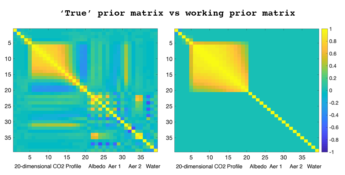
2.2. Working Prior vs. True Prior

Now, assume that we have two OE retrievals for ${\mathbf{y}}_1$ and ${\mathbf{y}}_2$ with priors $\{{\mathbf{x}}_{a,1},{\mathbf{S}}_{a,1}\}$ and $\{{\mathbf{x}}_{a,2},{\mathbf{S}}_{a,2}\}$, respectively, where $\{{\mathbf{x}}_{a,1},{\mathbf{S}}_{a,1}\}$ is generally different from $\{{\mathbf{x}}_{a,2},{\mathbf{S}}_{a,2}\}$, both of which are typically misspecified relative to the (unknown) natural variability parameters $\{{\mathbf{x}}_T,{\mathbf{S}}_T\}$. We note that in strictly Bayesian tradition, the prior is taken as a starting point or as an opinion, and hence, there is no preferred “true” prior. However, optimal estimation, as formalized by [3], recognizes that there is a true (but unobserved) natural distribution of $\mathbf{x}$ and that ${\mathbf{x}}_T$ and ${\mathbf{S}}_T$ are simply the first and second moments of this distribution (i.e., ${\mathbf{x}}_T=\mathrm{E}\left(\mathbf{x}\right)$ and ${\mathbf{S}}_T=\mathrm{var}\left(\mathbf{x}\right)$). It is also recognized that the prior used in the OE algorithm can be misspecified relative to this true prior [3], and he noted that “if the a priori are inappropriate, [then] their errors are incorrect.” He further acknowledged the difficulty of knowing the true prior $\{{\mathbf{x}}_T,{\mathbf{S}}_T\}$, recommending that in choosing a working prior that practitioners make a “reasonable estimate of a probability density function consistent with all our knowledge, one that is least committal about the state but consistent with whatever more or less detailed understanding we may have of the state vector prior to the measurement(s)” ([3] Section 10.3.3.2).

Following the framework in OE, there is clearly a preferred prior. This is evident in the existing literature, where the general consensus in prior design is to make the working prior as “accurate” as possible (e.g., [3,12,24]). For instance, Reference [24] noted that “[using] the most accurate prior will lead to the most accurate result.” Reference [13] showed that using the true prior $\{{\mathbf{x}}_T,{\mathbf{S}}_T\}$ in the OE algorithm will result in retrievals with the following properties: (1) unbiasedness, (2) smallest uncertainties (relative to $\mathbf{x}$) among all choices of priors, and (3) accurate posterior uncertainties. All of these properties are desirable in instrument design, validation, and scientific analysis. For this reason, we call $\{{\mathbf{x}}_T,{\mathbf{S}}_T\}$ the “true” prior, with the acknowledgment that in practice, the working prior is rarely, if ever, identical to the true prior.

Given the working priors, Reference [3] gave the following expression for the retrieved states ${\widehat{\mathbf{x}}}_1$ and ${\widehat{\mathbf{x}}}_2$:

$$\begin{array}{ccc}{\widehat{\mathbf{x}}}_1\hfill & =\hfill & {\mathbf{x}}_{a,1}+{({\mathbf{S}}_{a,1}^{-1}+{\mathbf{K}}_1^{\prime }{\mathbf{S}}_{ϵ,1}^{-1}{\mathbf{K}}_1)}^{-1}{\mathbf{K}}_1^{\prime }{\mathbf{S}}_{ϵ,1}^{-1}({\mathbf{y}}_1-{\mathbf{K}}_1{\mathbf{x}}_{a,1})\hfill \\ \hfill & =\hfill & {\mathbf{x}}_{a,1}+{\mathbf{A}}_1\mathbf{x}+{ϵ}_{r,1}-{\mathbf{A}}_1{\mathbf{x}}_{a,1},\hfill \end{array}$$

(3)

and similarly,

$$\begin{array}{ccc}\hfill {\widehat{\mathbf{x}}}_2& =& {\mathbf{x}}_{a,2}+{\mathbf{A}}_2\mathbf{x}+{ϵ}_{r,2}-{\mathbf{A}}_2{\mathbf{x}}_{a,2},\hfill \end{array}$$

(4)

where ${\mathbf{A}}_i={({\mathbf{S}}_{a,i}^{-1}+{\mathbf{K}}_i^{\prime }{\mathbf{S}}_{ϵ,i}^{-1}{\mathbf{K}}_i)}^{-1}{\mathbf{K}}_i^{\prime }{\mathbf{S}}_{ϵ,i}^{-1}{\mathbf{K}}_i$ is the averaging kernel, ${\mathbf{G}}_i={({\mathbf{S}}_{a,i}^{-1}+{\mathbf{K}}_i^{\prime }{\mathbf{S}}_{ϵ,i}^{-1}{\mathbf{K}}_i)}^{-1}{\mathbf{K}}_i^{\prime }{\mathbf{S}}_{ϵ,i}^{-1}$ is the gain matrix, and ${ϵ}_{r,i}={\mathbf{G}}_i{ϵ}_i$. For the ease of reference, we include a list of notations and their definitions in

Table 1. Reference guide for the mathematical symbols.

Symbol	Definition
${\mathbf{y}}_i$	Observed $N_i$-dimensional vector of radiances from the i-th instrument
$\mathbf{x}$	True (hidden) r-dimensional vector of state elements
${ϵ}_i$	$N_i$-dimensional vector of radiance error for the i-th instrument
${\mathbf{K}}_i$	Jacobian of the i-th forward model
${\mathbf{x}}_T$	True prior mean vector of the state vector $\mathbf{x}$
${\mathbf{x}}_{a,i}$	Working prior mean vector of $\mathbf{x}$ for the i-th retrieval
${\mathbf{x}}_C$	Comparison ensemble mean within averaging kernel correction
${\mathbf{S}}_{ϵ,i}$	Covariance matrix for the radiance measurement error of the i-th instrument
${\mathbf{S}}_T$	True prior covariance matrix of the state vector $\mathbf{x}$
${\mathbf{S}}_{a,i}$	Working prior covariance matrix of $\mathbf{x}$ for the i-th retrieval
${\mathbf{S}}_C$	Comparison ensemble covariance matrix within averaging kernel correction
${\mathbf{G}}_i$	Gain matrix computed with the prior $\{{\mathbf{x}}_{a,i},{\mathbf{S}}_{a,i}\}$
${\mathbf{A}}_i$	Averaging kernel computed with the prior $\{{\mathbf{x}}_{a,i},{\mathbf{S}}_{a,i}\}$
${\widehat{\mathbf{x}}}_i$	Retrieved state from ${\mathbf{y}}_i$ using the working prior $\{{\mathbf{x}}_{a,i},{\mathbf{S}}_{a,i}\}$
${\widehat{\mathbf{x}}}_{12}$	Averaging kernel adjusted ${\widehat{\mathbf{x}}}_2$ under the comparison ensemble $\{{\mathbf{x}}_{a,1},{\mathbf{S}}_{a,1}\}$

.

2.3. Relative Bias from Different OE Retrievals of the Same State

In general, using a prior that is different from the true prior will result in a bias. Reference [13] showed for a given retrieval with prior $\{{\mathbf{x}}_{a,i},{\mathbf{S}}_{a,i}\}$ that there is a bias given by:

$$\begin{array}{ccc}{\mathbf{b}}_i\hfill & \equiv \hfill & {\mathrm{E}}_T({\widehat{\mathbf{x}}}_i-\mathbf{x})\hfill \\ \hfill & =\hfill & {\mathrm{E}}_T({\mathbf{x}}_{a,i}+{\mathbf{G}}_i({\mathbf{y}}_i-{\mathbf{K}}_i{\mathbf{x}}_i)-\mathbf{x})\hfill \\ \hfill & =\hfill & (\mathbf{I}-{\mathbf{A}}_i)({\mathbf{x}}_{a,i}-{\mathbf{x}}_T)\hfill \\ \hfill & =\hfill & {({\mathbf{S}}_{a,i}^{-1}+{\mathbf{K}}_i^{\prime }{\mathbf{S}}_{ϵ}^{-1}{\mathbf{K}}_i)}^{-1}{\mathbf{S}}_{a,i}^{-1}({\mathbf{x}}_{a,i}-{\mathbf{x}}_T),\hfill \end{array}$$

(5)

where the subscript T on the expected value operator indicates that it is taken with respect to the true natural variability of the state and ${\mathbf{A}}_i\equiv {\mathbf{G}}_i{\mathbf{K}}_i$ is the working averaging kernel. Note that the equation above implies that it is possible for an instrument to have an incorrect prior mean, but still be unbiased if it uses an uninformative prior (that is, assuming that ${\mathbf{S}}_{a,i}$ is “large” enough that ${\mathbf{S}}_{a,i}^{-1}$ is effectively $\mathbf{0}$). However, most OE retrievals in remote sensing use an informative prior covariance matrix, since many retrieval problems are ill-posed, and there is not enough information to provide a unique solution (i.e., ${\mathbf{K}}^{\prime }{\mathbf{S}}_{ϵ}^{-1}\mathbf{K}$ is singular) without adding in constraints implied by the prior covariance matrix ${\mathbf{S}}_{a,i}$. Therefore, for the rest of this paper, we will assume that ${\mathbf{S}}_{a,i}<\infty$ (i.e., all eigenvalues of ${\mathbf{S}}_{a,i}$ are finite).

A simple corollary of Equation (5) is that whenever we compare two OE retrievals with different working prior means, the comparisons would be biased. The expected value of the difference between ${\widehat{\mathbf{x}}}_1$ and ${\widehat{\mathbf{x}}}_2$ is:

$$\begin{array}{ccc}{\mathrm{E}}_T({\widehat{\mathbf{x}}}_1-{\widehat{\mathbf{x}}}_2)\hfill & =\hfill & {\mathrm{E}}_T({\widehat{\mathbf{x}}}_1-\mathbf{x})-{\mathrm{E}}_T({\widehat{\mathbf{x}}}_2-\mathbf{x})\hfill \\ \hfill & =\hfill & (\mathbf{I}-{\mathbf{A}}_1)({\mathbf{x}}_{a,1}-{\mathbf{x}}_T)-(\mathbf{I}-{\mathbf{A}}_2)({\mathbf{x}}_{a,2}-{\mathbf{x}}_T),\hfill \end{array}$$

(6)

It is easy to see from Equation (6) that two retrievals with different working prior mean vectors (i.e., ${\mathbf{x}}_{a,1}\ne {\mathbf{x}}_{a,2})$ in general will have a relative bias. Even if the working prior mean vectors are the same, it is still possible for ${\mathrm{E}}_T({\widehat{\mathbf{x}}}_1-{\widehat{\mathbf{x}}}_2)\ne \mathbf{0}$ if either ${\mathbf{S}}_{a,1}\ne {\mathbf{S}}_{a,2}$ or ${\mathbf{K}}_1\ne {\mathbf{K}}_2$, since they imply that ${\mathbf{A}}_1\ne {\mathbf{A}}_2$. Another somewhat unintuitive result is that there is also a relative bias if data from the two different instruments are retrieved with identical forward models, prior mean vectors, and prior covariance matrices. This is because the two instruments will have different measurement error characteristics (i.e., ${\mathbf{S}}_{ϵ,1}\ne {\mathbf{S}}_{ϵ,2}$). Since the definition of the averaging kernel includes a term for ${\mathbf{S}}_{ϵ,i}$, this implies that ${\mathbf{A}}_1\ne {\mathbf{A}}_2$ even when $\{{\mathbf{x}}_{a,1},{\mathbf{S}}_{a,1}\}=\{{\mathbf{x}}_{a,2},{\mathbf{S}}_{a,2}\}$. This in turn implies that ${\mathrm{E}}_T({\widehat{\mathbf{x}}}_1-{\widehat{\mathbf{x}}}_2)\ne \mathbf{0}.$

2.4. Averaging Kernel Correction

It has been long recognized that the comparison of OE retrievals with different priors is susceptible to prior-induced biases (e.g., [20,22]). The definitive treatment of this topic was given in [20], which describes how to compare retrievals with different OE priors by shifting each of the retrievals involved onto a common prior $\{{\mathbf{x}}_C,{\mathbf{S}}_C\}$, which Reference [20] called the “comparison ensemble”. While Reference [20] did not imply that their procedure would ensure unbiasedness, a general misconception in the remote sensing literature is that the prior-induced bias implied by Equation (6) can be removed by the averaging kernel convolution process (e.g., [21]). Specifically, the misconception is that given two OE retrievals ${\widehat{\mathbf{x}}}_1$ and ${\widehat{\mathbf{x}}}_2$ from two different priors, if one adjusts ${\widehat{\mathbf{x}}}_2$ into ${\widehat{\mathbf{x}}}_{12}$ by convolving with the averaging kernel, then the relative bias between ${\widehat{\mathbf{x}}}_1$ and the averaging kernel-corrected ${\widehat{\mathbf{x}}}_{12}$ is zero; that is, $\mathrm{E}({\widehat{\mathbf{x}}}_{12}-{\widehat{\mathbf{x}}}_1)=\mathbf{0}$. However, we will show analytically that this claim is not supported by the paper [20].

In applications of averaging kernel correction, it is common to choose the comparison ensemble from one of the two priors used to produce the datasets. One advantage of this approach is that the researcher doing the intercomparison can take advantage of the subject matter expertise as encoded in the existing priors, although it is prudent for the researcher to select the prior that is considered more accurate or precise from the two as the comparison ensemble. Another advantage of this approach, of course, is that the retrievals from the dataset with the chosen comparison prior do not need any adjustment. For instance, when comparing OCO-2 retrievals to TCCON retrievals, one might adjust the OCO-2 retrievals using the TCCON averaging kernel while leaving TCCON retrievals unadjusted (e.g., [14]).

Here, without loss of generality, we will choose the prior $\{{\mathbf{x}}_{a,1},{\mathbf{S}}_{a,1}\}$ as the comparison ensemble. That is, we set $\{{\mathbf{x}}_C,{\mathbf{S}}_C\}=\{{\mathbf{x}}_{a,1},{\mathbf{S}}_{a,1}\}$. This implies that we need to adjust ${\widehat{\mathbf{x}}}_2$. From [20], the general procedure for this averaging kernel correction process is as follows:

• Add an adjustment term $({\mathbf{A}}_2-\mathbf{I})({\mathbf{x}}_{a,2}-{\mathbf{x}}_{a,1})$ to ${\widehat{\mathbf{x}}}_2$ to shift the prior mean ([20] Section 3).
• Make ${\widehat{\mathbf{x}}}_2$ “optimal” with respect to the comparison ensemble $\{{\mathbf{x}}_{a,1},{\mathbf{S}}_{a,1}\}$ ([20] Equation (18)).
• Simulate the profile of ${\widehat{\mathbf{x}}}_1$ by modifying ${\widehat{\mathbf{x}}}_2$ ([20] Equation (28)).

Combining Steps 1 to 3 above, the adjusted value ${\widehat{\mathbf{x}}}_{12}$ is given as follows:

$$\begin{array}{ccc}{\widehat{\mathbf{x}}}_{12}\hfill & =\hfill & {\mathbf{x}}_{a,1}+{\mathbf{A}}_1{\mathbf{S}}_{a,1}{\mathbf{A}}_2^{\prime }{\left({\mathbf{A}}_2{\mathbf{S}}_{a,1}{\mathbf{A}}_2^{\prime }+{\mathbf{G}}_2{\mathbf{S}}_{ϵ,2}{\mathbf{G}}_2^{\prime }\right)}^{-1}\hfill \\ \hfill & \hfill & ·({\widehat{\mathbf{x}}}_2+({\mathbf{A}}_2-\mathbf{I})({\mathbf{x}}_{a,2}-{\mathbf{x}}_{a,1})-{\mathbf{x}}_{a,1})\hfill \\ \hfill & =\hfill & {\mathbf{x}}_{a,1}+{\mathbf{A}}_1{\mathbf{S}}_{a,1}{\mathbf{A}}_2^{\prime }{\left({\mathbf{A}}_2{\mathbf{S}}_{a,1}{\mathbf{A}}_2^{\prime }+{\mathbf{G}}_2{\mathbf{S}}_{ϵ,2}{\mathbf{G}}_2^{\prime }\right)}^{-1}\hfill \\ \hfill & \hfill & ·({\mathbf{A}}_2\mathbf{x}+{ϵ}_{r,2}-{\mathbf{A}}_2{\mathbf{x}}_{a,1}).\hfill \end{array}$$

(7)

We note that in a particular variant of averaging kernel correction, Step 2 (making ${\widehat{\mathbf{x}}}_2$ optimal with respect to the comparison ensemble) is skipped in the process (e.g., [22]). This should only be done when the retrieval to be modified is already optimal with respect to the comparison ensemble $\{{\mathbf{x}}_C,{\mathbf{S}}_C\}$. As [20], Section 4.4, noted, “if retrieval 2 is not optimal with respect to the comparison ensemble, then Equation (18) [denoted in this paper as Step 2 in the itemized list above] should be used to convert it, and to provide an improved averaging kernel matrix.” In this paper, we assume that the full averaging kernel correction is performed as suggested by [20], although the majority of our conclusions (with one important exception) still apply to the abbreviated averaging kernel correction variant in [22] (see Section 2.6 for more details).

2.5. Examining the Biases

Having set up the background and the appropriate convolution with the averaging kernel, we will examine the biases that arise therefrom. First, let us consider the bias of ${\widehat{\mathbf{x}}}_1$ relative to the unobserved truth $\mathbf{x}$. Since we used $\{{\mathbf{x}}_{a,1},{\mathbf{S}}_{a,1}\}$ as the comparison ensemble, no adjustment to ${\widehat{\mathbf{x}}}_1$ is necessary. From [13], this bias is equal to:

$$\begin{array}{c}\hfill \mathrm{E}({\widehat{\mathbf{x}}}_1-\mathbf{x})=({\mathbf{A}}_1-\mathbf{I})({\mathbf{x}}_T-{\mathbf{x}}_{a,1}).\end{array}$$

(8)

It is also straightforward to show that the adjusted value ${\widehat{\mathbf{x}}}_{12}$ given in Equation (7) is also biased relative to the truth:

$$\begin{array}{ccc}\mathrm{E}({\widehat{\mathbf{x}}}_{12}-\mathbf{x})\hfill & =\hfill & \mathrm{E}({\mathbf{x}}_{a,1}+{\mathbf{A}}_1{\mathbf{S}}_{a,1}{\mathbf{A}}_2^{\prime }{\left({\mathbf{A}}_2{\mathbf{S}}_{a,1}{\mathbf{A}}_2^{\prime }+{\mathbf{G}}_2{\mathbf{S}}_{ϵ,2}{\mathbf{G}}_2^{\prime }\right)}^{-1}\hfill \\ \hfill & \hfill & ·({\mathbf{A}}_2\mathbf{x}+{ϵ}_{r,2}-{\mathbf{A}}_2{\mathbf{x}}_{a,1})-\mathbf{x})\hfill \\ \hfill & =\hfill & {\mathbf{x}}_{a,1}+{\mathbf{A}}_1{\mathbf{S}}_{a,1}{\mathbf{A}}_2^{\prime }{\left({\mathbf{A}}_2{\mathbf{S}}_{a,1}{\mathbf{A}}_2^{\prime }+{\mathbf{G}}_2{\mathbf{S}}_{ϵ,2}{\mathbf{G}}_2^{\prime }\right)}^{-1}\hfill \\ \hfill & \hfill & ·({\mathbf{A}}_2{\mathbf{x}}_T-{\mathbf{A}}_2{\mathbf{x}}_{a,1})-{\mathbf{x}}_T\hfill \\ \hfill & =\hfill & ({\mathbf{A}}_1{\mathbf{S}}_{a,1}{\mathbf{A}}_2^{\prime }{\left({\mathbf{A}}_2{\mathbf{S}}_{a,1}{\mathbf{A}}_2^{\prime }+{\mathbf{G}}_2{\mathbf{S}}_{ϵ,2}{\mathbf{G}}_2^{\prime }\right)}^{-1}{\mathbf{A}}_2-\mathbf{I})({\mathbf{x}}_T-{\mathbf{x}}_{a,1}).\hfill \end{array}$$

(9)

Finally, we show that the retrieval ${\widehat{\mathbf{x}}}_1$ and the adjusted retrieval ${\widehat{\mathbf{x}}}_{12}$ are also biased relative to one another. That is,

$$\begin{array}{ccc}\mathrm{E}({\widehat{\mathbf{x}}}_{12}-{\widehat{\mathbf{x}}}_1)\hfill & =\hfill & \mathrm{E}({\mathbf{x}}_{a,1}+{\mathbf{A}}_1{\mathbf{S}}_{a,1}{\mathbf{A}}_2^{\prime }\left({\mathbf{A}}_2{\mathbf{S}}_{a,1}{\mathbf{A}}_2^{\prime }+{\mathbf{G}}_2{\mathbf{S}}_{ϵ,2}^{-1}{\mathbf{G}}_2^{\prime }\right)\hfill \\ \hfill & \hfill & ·({\mathbf{A}}_2\mathbf{x}+{ϵ}_{r,2}-{\mathbf{A}}_2{\mathbf{x}}_{a,1})-{\mathbf{x}}_{a,1}-{\mathbf{A}}_1\mathbf{x}-{ϵ}_{r,1}+{\mathbf{A}}_1{\mathbf{x}}_{a,1})\hfill \\ \hfill & =\hfill & {\mathbf{A}}_1{\mathbf{S}}_{a,1}{\mathbf{A}}_2^{\prime }{\left({\mathbf{A}}_2{\mathbf{S}}_{a,1}{\mathbf{A}}_2^{\prime }+{\mathbf{G}}_2{\mathbf{S}}_{ϵ,2}{\mathbf{G}}_2^{\prime }\right)}^{-1}{\mathbf{A}}_2({\mathbf{x}}_T-{\mathbf{x}}_{a,1})\hfill \\ \hfill & \hfill & -{\mathbf{A}}_1({\mathbf{x}}_T-{\mathbf{x}}_{a,1})\hfill \\ \hfill & =\hfill & ({\mathbf{A}}_1{\mathbf{S}}_{a,1}{\mathbf{A}}_2^{\prime }{\left({\mathbf{A}}_2{\mathbf{S}}_{a,1}{\mathbf{A}}_2^{\prime }+{\mathbf{G}}_2{\mathbf{S}}_{ϵ,2}{\mathbf{G}}_2^{\prime }\right)}^{-1}{\mathbf{A}}_2-{\mathbf{A}}_1)({\mathbf{x}}_T-{\mathbf{x}}_{a,1}).\hfill \end{array}$$

(10)

The result in Equation (10) is particularly concerning for instrument validation in practice, because it implies that even after implementing the averaging kernel correction as suggested by [20], there is still a relative bias that is proportional to $({\mathbf{x}}_T-{\mathbf{x}}_C)$, and this bias arises solely from the misspecification of the comparison ensemble $\{{\mathbf{x}}_C,{\mathbf{S}}_C\}$.

For instance, OCO-2 retrievals are often compared to TCCON retrievals (after the appropriate averaging kernel adjustments) in order to assess the relative bias. The result in Equation (10) indicates that such a comparison will produce a bias as long as the comparison ensemble is not the same as the natural variability of the state $\mathbf{x}$ (i.e., ${\mathbf{x}}_T\ne {\mathbf{x}}_C$). In other words, a comparison between OCO-2 retrievals and TCCON might produce a bias that might lead the OCO-2 instrument team to re-examine issues such as calibration and absorption coefficients, when the bias is actually due to the comparison profile not being the same as the true mean of the state. In this case, where ${\mathbf{x}}_T\ne {\mathbf{x}}_C$, chasing after calibration or spectroscopy to remove the bias would be fruitless.

In some validation exercises, it might be important to assess the relative magnitude of the prior-induced bias relative to known validation errors, and Equation (10) offers a means to do so. Note that Equation (10) only has one unknown, which is the true prior means ${\mathbf{x}}_T$. Here, the researcher can make reasonable guesses at some choices of ${\mathbf{x}}_T$ and then compute what would be the resulting prior-induced biases. For instance, the researcher may assume that ${\mathbf{x}}_C$ is misspecified by 1% or 2% (i.e., ${\mathbf{x}}_C=0.99{\mathbf{x}}_T$ or ${\mathbf{x}}_C=0.98{\mathbf{x}}_T$), which can then be used in Equation (10) to produce a numeric result that the researcher can compare to other sources of error.

Upon closer examination of the biases in Equations (8)–(10), we see that they all involve a multiplicative term $({\mathbf{x}}_T-{\mathbf{x}}_C)$, where recall that for this particular example, we set $\{{\mathbf{x}}_C,{\mathbf{S}}_C\}=\{{\mathbf{x}}_{a,1},{\mathbf{S}}_{a,1}\}$. It is then easy to see where the misunderstanding about the convolution of the averaging kernel being able to remove the bias originated, since if ${\mathbf{x}}_T={\mathbf{x}}_C$, then it is obvious that $\mathrm{E}({\widehat{\mathbf{x}}}_1-\mathbf{x})=\mathbf{0}$, $\mathrm{E}({\widehat{\mathbf{x}}}_{12}-\mathbf{x})=\mathbf{0}$ and $\mathrm{E}({\widehat{\mathbf{x}}}_{12}-{\widehat{\mathbf{x}}}_1)=\mathbf{0}$. That is, the general misconception in the literature arises from the implicit assumption that the comparison prior means ${\mathbf{x}}_C$ is equal to the true prior means ${\mathbf{x}}_T$. Reference [20] described how to compare retrievals with different priors by moving the retrievals onto a common comparison ensemble $\{{\mathbf{x}}_C,{\mathbf{S}}_C\}$, but their paper did not address what happens when this comparison ensemble mean ${\mathbf{x}}_C$ is different from the true mean ${\mathbf{x}}_T$ of the state $\mathbf{x}$.

Unfortunately for OE retrievals, the comparison profile is almost certainly not equal to $\{{\mathbf{x}}_T,{\mathbf{S}}_T\}$ in real applications. This leads to biases in $\mathrm{E}({\widehat{\mathbf{x}}}_1-\mathbf{x})$, $\mathrm{E}({\widehat{\mathbf{x}}}_{12}-\mathbf{x})$, and $\mathrm{E}({\widehat{\mathbf{x}}}_{12}-{\widehat{\mathbf{x}}}_1)$, and this is why it is important to consider the effect of prior misspecification. In instrument team validation, it is often necessary to compare OE retrievals to retrievals from a validation source in order to assess the bias. Often, an averaging kernel correction is applied before intercomparison, and the instrument team would attempt to correlate any resulting bias with potential sources (e.g., spectroscopy, calibration, clouds and aerosols, etc.). The result in Equation (10) indicates that the choice of priors should be considered as a potential source of bias whenever intercomparison between multiple retrievals is necessary (e.g., instrument validation, data assimilation of multiple data sources, etc.).

It is important to note that the relative bias in Equation (10) will change depending on the choice of the comparison prior. That is, in general, $\mathrm{E}({\widehat{\mathbf{x}}}_{12}-{\widehat{\mathbf{x}}}_1)\ne \mathrm{E}({\widehat{\mathbf{x}}}_{21}-{\widehat{\mathbf{x}}}_2)$. In many applications, a researcher is given two different OE retrievals and has the choice of selecting one of the two corresponding priors as the comparison prior. Here, the researcher may not be able to avoid a relative bias via the averaging kernel correction process, but he or she might be able to reduce its effect by selecting the prior that results in a smaller bias.

We first note that the biases in Equations (8)–(10) and Equation (10) are all proportional to $({\mathbf{x}}_T-{\mathbf{x}}_C)$. Therefore, if possible, from the two choices, a researcher should select the one that has a more realistic prior mean; that is, a prior mean that is more likely to be close to the true hidden prior mean, which would then reduce the magnitude of the term $({\mathbf{x}}_T-{\mathbf{x}}_C)$.

In some applications, however, it is not easy to judge which of the two prior means is more realistic or more accurate. In this case, it is possible to rely on the choice of the prior covariance matrix ${\mathbf{S}}_C$ to mitigate the magnitude of the prior-induced bias. It has been demonstrated that using a “large” prior covariance matrix in an OE algorithm will reduce the magnitude of the prior-induced bias [13]. This is because inflating the prior covariance matrix will decrease the information content of the prior, thereby reducing the magnitude to which a misspecified prior mean can bias the retrieval.

In the same manner, choosing a “larger” covariance matrix for ${\mathbf{S}}_C$ will decrease the magnitude of $\mathrm{E}({\widehat{\mathbf{x}}}_1-\mathbf{x})$, $\mathrm{E}({\widehat{\mathbf{x}}}_{12}-\mathbf{x})$, and $\mathrm{E}({\widehat{\mathbf{x}}}_{12}-{\widehat{\mathbf{x}}}_1)$. Let us consider the limiting case where ${\mathbf{S}}_C={\mathbf{S}}_{a,1}\to \infty$. Since the averaging kernel is given as ${\mathbf{A}}_1={({\mathbf{S}}_{a,1}^{-1}+\mathbf{K}{\mathbf{S}}_{ϵ,1}^{-1}{\mathbf{K}}^{\prime })}^{-1}{\mathbf{K}}^{\prime }{\mathbf{S}}_{ϵ,1}^{-1}\mathbf{K}$, then ${\mathbf{A}}_1\to \mathbf{I}$ as ${\mathbf{S}}_{a,1}\to \infty$, and it is easy to see that,

$$\begin{array}{ccc}\hfill \underset{{\mathbf{S}}_{a,1}\to \infty }{lim}\mathrm{E}({\widehat{\mathbf{x}}}_1-\mathbf{x})& =& ({\mathbf{A}}_1-\mathbf{I})({\mathbf{x}}_T-{\mathbf{x}}_{a,1})\hfill \\ & =& (\mathbf{I}-\mathbf{I})({\mathbf{x}}_T-{\mathbf{x}}_{a,1})\hfill \\ & =& \mathbf{0}.\hfill \end{array}$$

Likewise, we can show the same result for the averaging kernel-corrected ${\widehat{\mathbf{x}}}_{12}$ as well,

$$\begin{array}{ccc}\underset{{\mathbf{S}}_{a,1}\to \infty }{lim}\mathrm{E}({\widehat{\mathbf{x}}}_{12}-\mathbf{x})\hfill & =\hfill & ({\mathbf{A}}_1{\mathbf{S}}_{a,1}{\mathbf{A}}_2^{\prime }{\left({\mathbf{A}}_2{\mathbf{S}}_{a,1}{\mathbf{A}}_2^{\prime }+{\mathbf{G}}_2{\mathbf{S}}_{ϵ,2}{\mathbf{G}}_2^{\prime }\right)}^{-1}{\mathbf{A}}_2-\mathbf{I})({\mathbf{x}}_T-{\mathbf{x}}_{a,1})\hfill \\ \hfill & =\hfill & ({\mathbf{A}}_1{\mathbf{S}}_{a,1}{\mathbf{A}}_2^{\prime }{\left({\mathbf{A}}_2{\mathbf{S}}_{a,1}{\mathbf{A}}_2^{\prime }\right)}^{-1}{\mathbf{A}}_2-\mathbf{I})({\mathbf{x}}_T-{\mathbf{x}}_{a,1})\hfill \\ \hfill & =\hfill & ({\mathbf{A}}_1-\mathbf{I})({\mathbf{x}}_T-{\mathbf{x}}_{a,1})\hfill \\ \hfill & =\hfill & \mathbf{0}.\hfill \end{array}$$

(11)

Following the procedure above, it is easy to show that the relative bias $\mathrm{E}({\widehat{\mathbf{x}}}_{12}-{\widehat{\mathbf{x}}}_1)\to \mathbf{0}$ as the comparison prior covariance matrix ${\mathbf{S}}_C\to \infty$. Therefore, if minimizing the relative bias is of paramount concern and a researcher is unsure of the accuracy of the prior means ${\mathbf{x}}_{a,1}$ and ${\mathbf{x}}_{a,2}$, it is a good idea to choose a prior with a “larger” prior covariance matrix as the comparison prior. This result also provides for an avenue for completely removing the prior-induced bias in the intercomparison of OE priors. If it is absolutely important to remove the prior as a source of bias in a validation study, one approach would be to let ${\mathbf{S}}_C$ be an uninformative matrix (i.e., ${\mathbf{S}}_C\to \infty$), which would force the prior-induced bias to approach zero. It is important to note, however, that there are some trade-offs involved in using a less informative prior covariance matrix. For instance, when the instrument signal-to-noise ratio is low, using an uninformative prior covariance can result in very large posterior uncertainties (for more details, see [13]). In the case of averaging kernel corrections, letting ${\mathbf{S}}_C\to \infty$ will ensure that $\mathrm{E}({\widehat{\mathbf{x}}}_{12}-{\widehat{\mathbf{x}}}_1)\to \mathbf{0}$, but this choice may lead to larger variability in the difference (i.e., $\mathrm{var}({\widehat{\mathbf{x}}}_{12}-{\widehat{\mathbf{x}}}_1)$ may be “larger”).

At this point, the reader may ask if Equation (6) points at a possible approach to estimate the true prior mean vector ${\mathbf{x}}_T$. That is, given a set of retrievals and the fact that the bias is proportional to $({\mathbf{x}}_C-{\mathbf{x}}_T)$, we can iterate over different choices of ${\mathbf{x}}_C$ until we achieve $\mathrm{E}({\widehat{\mathbf{x}}}_{12}-{\widehat{\mathbf{x}}}_1)=\mathbf{0}$, which should occur when ${\mathbf{x}}_C={\mathbf{x}}_T$. In theory, this is possible. However, recall that in this paper, we simplified the problem to assume no bias from non-prior sources (e.g., calibration, spectroscopy, geolocation, interference factors such as aerosols, etc.). In real applications, the prior-induced bias is likely only one component of the overall bias, and iterating ${\mathbf{x}}_C$ until $\mathrm{E}({\widehat{\mathbf{x}}}_{12}-{\widehat{\mathbf{x}}}_1)=\mathbf{0}$ would then falsely ascribe these non-prior sources of bias to the choice of the comparison ensemble. A more principled approach would be to try to remove the prior-induced bias via the recommendations in this section, which would allow the researcher to be reasonably sure that any bias remaining is due to other causes such as calibration or spectroscopy.

In this section, we consider the biases in the original state vector space. In many applications, the state vector is convolved into a scalar using a linear weight vector (e.g., combining the 20-dimensional CO₂ vector into an XCO2 value [25]). That is, given a state vector $\mathbf{x}$, it is converted into a scalar as a linear combination $x={\mathbf{h}}^{\prime }\mathbf{x}$, where $\mathbf{h}$ is a pressure weighting vector. It is easy to see that the scalar bias can be easily computed from the results in Equations (8)–(10). For instance, for a given pressure weight vector $\mathbf{h}$, the scalar relative bias $\mathrm{E}({\widehat{x}}_{12}-{\widehat{x}}_1)$ is given as follows:

$$\begin{array}{ccc}\mathrm{E}({\widehat{x}}_{12}-{\widehat{x}}_1)\hfill & =\hfill & \mathrm{E}({\mathbf{h}}^{\prime }{\widehat{\mathbf{x}}}_{12}-{\mathbf{h}}^{\prime }{\widehat{\mathbf{x}}}_1)\hfill \\ \hfill & =\hfill & {\mathbf{h}}^{\prime }\mathrm{E}({\widehat{\mathbf{x}}}_{12}-{\widehat{\mathbf{x}}}_1).\hfill \end{array}$$

(12)

We note that most of the conclusions in this section will hold in the scalar space, although the magnitude of the scalar bias will vary depending on the choice of the weight vector $\mathbf{h}$. In theory, it is possible for $\mathbf{h}$ to be orthogonal to $\mathrm{E}({\widehat{\mathbf{x}}}_{12}-{\widehat{\mathbf{x}}}_1)$, which would result in the scalar bias being zero. In practice, the weighting vector is often constructed based on physical motivations (e.g., [25]), independent of the prior selection process. Therefore, it is nearly impossible for these two vectors to be orthogonal, and it would be foolhardy to rely on this infinitesimally small chance as a means to remove this prior-induced bias.

2.6. Abbreviated Variant of Averaging Kernel Correction

As we noted earlier, a variant of the averaging kernel correction process omits Step 2 (adjusting retrievals to make them “optimal” relative to $\{{\mathbf{x}}_C,{\mathbf{S}}_C\}$) of the procedure on Line 217. Reference [20] recommended that Step 2 be taken whenever the retrievals to be compared have a different prior than $\{{\mathbf{x}}_C,{\mathbf{S}}_C\}$, but this advice is not always heeded in practice. In this variant, the abbreviated averaging kernel correction has a much simpler form:

$$\begin{array}{ccc}{\widehat{\mathbf{x}}}_{12}\hfill & =\hfill & {\mathbf{x}}_{a,1}+{\mathbf{A}}_1({\widehat{\mathbf{x}}}_2+({\mathbf{A}}_2-\mathbf{I})({\mathbf{x}}_{a,2}-{\mathbf{x}}_{a,1})-{\mathbf{x}}_{a,1})\hfill \\ \hfill & =\hfill & {\mathbf{x}}_{a,1}+{\mathbf{A}}_1({\mathbf{A}}_2\mathbf{x}+{ϵ}_{r,2}-{\mathbf{A}}_2{\mathbf{x}}_{a,1}).\hfill \end{array}$$

(13)

The relative bias $\mathrm{E}({\widehat{\mathbf{x}}}_{12}-{\widehat{\mathbf{x}}}_1)$ is given as:

$$\begin{array}{ccc}\mathrm{E}({\widehat{\mathbf{x}}}_{12}-{\widehat{\mathbf{x}}}_1)\hfill & =\hfill & \mathrm{E}({\mathbf{x}}_{a,1}+{\mathbf{A}}_1({\mathbf{A}}_2\mathbf{x}+{ϵ}_{r,2}-{\mathbf{A}}_2{\mathbf{x}}_{a,1})-{\mathbf{x}}_{a,1}-{\mathbf{A}}_1\mathbf{x}-{ϵ}_{r,1}+{\mathbf{A}}_1{\mathbf{x}}_{a,1})\hfill \\ \hfill & =\hfill & {\mathbf{A}}_1({\mathbf{A}}_2-\mathbf{I})({\mathbf{x}}_T-{\mathbf{x}}_{a,1}).\hfill \end{array}$$

(14)

From Equation (14), we see that this abbreviated averaging kernel correction still has a relative bias if ${\mathbf{x}}_T\ne {\mathbf{x}}_C$ and that choosing a comparison prior mean that is as close as possible to ${\mathbf{x}}_C$ will reduce this prior-induced bias. However, we note that one important difference between Equations (6) and (14) is their behavior as ${\mathbf{S}}_C\to \infty$. We have seen that under the full averaging kernel correction in [20], making ${\mathbf{S}}_C$ more uninformative will reduce the prior-induced bias to $\mathbf{0}$. Under the abbreviated variant discussed in this section, this remedy is no longer available. This is because from Equation (14), it is easy to see that ${lim}_{{\mathbf{S}}_C\to \infty }\mathrm{E}({\widehat{\mathbf{x}}}_{12}-{\widehat{\mathbf{x}}}_1)=({\mathbf{A}}_2-\mathbf{I})({\mathbf{x}}_T-{\mathbf{x}}_{a,1})$. Therefore, we recommend that the averaging kernel correction follows the full procedure as described in [20] whenever possible.

2.7. Observation-Model Intercomparisons

In the previous section, we primarily studied the intercomparison of two OE retrievals, ${\widehat{\mathbf{x}}}_1$ and ${\widehat{\mathbf{x}}}_2$. In some applications, it is necessary to compare a remote sensing retrieval ${\widehat{\mathbf{x}}}_1$ against model data ${\widehat{\mathbf{x}}}_m$ (e.g., comparing GEOS-Chemchemical transport model data against satellite retrievals [26]). Further, for retrieval ${\widehat{\mathbf{x}}}_1$ and model data ${\widehat{\mathbf{x}}}_m$ in data assimilation, it is common to convolve the model profile with the averaging kernel of ${\widehat{\mathbf{x}}}_1$ using the following equation given by [27]:

$$\begin{array}{c}\hfill {\widehat{\mathbf{x}}}_{1m}={\mathbf{x}}_{a,1}+{\mathbf{A}}_1({\widehat{\mathbf{x}}}_m-{\mathbf{x}}_{a,1}).\end{array}$$

(15)

It is not immediately clear how the prior-induced bias would come into play, but a close inspection indicates that it comes from the misspecification in $\{{\mathbf{x}}_{a,1},{\mathbf{S}}_{a,1}\}$ and from biases in the model data.

We first assume that the model data ${\widehat{\mathbf{x}}}_m$ can be written as a function of the true value $\mathbf{x}$ in the following linear form:

$$\begin{array}{c}\hfill {\widehat{\mathbf{x}}}_m=\mathbf{b}+\mathbf{H}\mathbf{x}+\delta ,\end{array}$$

(16)

where $\mathbf{b}$ is an intercept term, $\mathbf{H}$ is the “slope” or a “scaling factor” on $\mathbf{x}$, and $\delta$ is a zero-mean residual error term. We can think of the model in Equation (16) as a first-order Taylor expansion of the functional relationship between ${\widehat{\mathbf{x}}}_m$ and the true state $\mathbf{x}$ where $\mathbf{b}$ and $\mathbf{H}$ are fixed parameters and $\delta$ is a random error vector. In theory, it is possible for the error term $\delta$ to have a non-zero mean, but that systematic error could be absorbed into the intercept term $\mathbf{b}$, so we will work with the simple zero-mean model.

Given the above, the bias of the corrected model profile ${\widehat{\mathbf{x}}}_{1m}$, relative to the true $\mathbf{x}$, is given as follows:

$$\begin{array}{ccc}\hfill \mathrm{E}({\widehat{\mathbf{x}}}_{1m}-\mathbf{x})& =& \mathrm{E}({\mathbf{x}}_{a,1}+{\mathbf{A}}_1({\widehat{\mathbf{x}}}_m-{\mathbf{x}}_{a,1})-\mathbf{x})\hfill \\ & =& \mathrm{E}({\mathbf{x}}_{a,1}+{\mathbf{A}}_1(\mathbf{b}+\mathbf{H}\mathbf{x}+\delta -{\mathbf{x}}_{a,1})-\mathbf{x})\hfill \\ & =& (\mathbf{I}-{\mathbf{A}}_1){\mathbf{x}}_{a,1}+{\mathbf{A}}_1\mathbf{b}+{\mathbf{A}}_1\mathbf{H}{\mathbf{x}}_T-{\mathbf{x}}_T\hfill \\ & =& (\mathbf{I}-{\mathbf{A}}_1){\mathbf{x}}_{a,1}+{\mathbf{A}}_1\mathbf{b}-(\mathbf{I}-{\mathbf{A}}_1\mathbf{H}){\mathbf{x}}_T,\hfill \end{array}$$

which indicates that when ${\mathbf{x}}_{a,1}\ne {\mathbf{x}}_T$, $\mathbf{b}\ne \mathbf{0}$ or $\mathbf{H}\ne \mathbf{I}$, then the bias $\mathrm{E}({\widehat{\mathbf{x}}}_{1m}-\mathbf{x})$ is generally nonzero. Similarly, if the goal is the intercomparison of the retrieved ${\widehat{\mathbf{x}}}_1$ against the corrected model data ${\widehat{\mathbf{x}}}_{1m}$, then we see that:

$$\begin{array}{ccc}\mathrm{E}({\widehat{\mathbf{x}}}_{1m}-{\widehat{\mathbf{x}}}_1)\hfill & =\hfill & \mathrm{E}({\mathbf{x}}_{a,1}+{\mathbf{A}}_1({\widehat{\mathbf{x}}}_m-{\mathbf{x}}_{a,1})-({\mathbf{x}}_{a,1}+{\mathbf{A}}_1\mathbf{x}+{ϵ}_{r,1}-{\mathbf{A}}_1{\mathbf{x}}_{a,1}))\hfill \\ \hfill & =\hfill & {\mathbf{x}}_{a,1}+{\mathbf{A}}_1\mathbf{b}+{\mathbf{A}}_1\mathbf{H}{\mathbf{x}}_T-{\mathbf{A}}_1{\mathbf{x}}_{a,1}-{\mathbf{x}}_{a,1}-{\mathbf{A}}_1{\mathbf{x}}_T+{\mathbf{A}}_1{\mathbf{x}}_{a,1}\hfill \\ \hfill & =\hfill & {\mathbf{A}}_1\mathbf{b}+{\mathbf{A}}_1(\mathbf{H}-\mathbf{I}){\mathbf{x}}_T.\hfill \end{array}$$

(17)

The result in Equation (17) is very interesting in that the effect of the prior means of ${\widehat{\mathbf{x}}}_1$ has disappeared entirely!That is, the prior mean ${\mathbf{x}}_{a,1}$ has disappeared from the expression for the bias. This is encouraging, especially when retrievals from multiple satellites are compared to the same model data. However, we note that the choice of the prior covariance ${\mathbf{S}}_{a,1}$ can still impact the magnitude of the bias, since the averaging kernel ${\mathbf{A}}_1$ appears as multiplicative factors on the right-hand side of Equation (17).

What is remarkable about the correction in Equation (17) is that the bias $\mathrm{E}({\widehat{\mathbf{x}}}_{1m}-{\widehat{\mathbf{x}}}_1)$ only depends on the intercept $\mathbf{b}$ and the Jacobian $\mathbf{H}$ of the first-order linear approximation of the functional relationship between ${\widehat{\mathbf{x}}}_m$ and the true state $\mathbf{x}$. It is obvious that if $\mathbf{b}=\mathbf{0}$ and $\mathbf{H}=\mathbf{I}$, then the observation-model intercomparison would be unbiased. However, this is essentially assuming that ${\widehat{\mathbf{x}}}_m=\mathbf{x}+\delta$ or that the model data are simply equal to the true state $\mathbf{x}$ plus some random zero-mean error. This is a very strong assumption and in general should require strong evidence for support.

It is important to note that although model data are often used as a proxy for the truth in remote sensing, they are not the same thing. In real practice, there likely would be some discrepancy between the model data and the true state $\mathbf{x}$, formalized by $\mathbf{b}\ne \mathbf{0}$ or $\mathbf{H}\ne \mathbf{I}$. In this case, the first-order Taylor approximation indicates that there would be a non-zero bias in the observation-model comparison!

In practice, the results in this section imply that researchers should generally be more skeptical in treating model data as a proxy for the truth. Often, any bias found in a observation-model intercomparison is ascribed to some potential causes in the retrievals (e.g., spectroscopy, calibration, systematic measurement errors, retrieval parameterizations, etc.). Equation (17) indicates that a bias might arise if the model data are “different” from the true field (that is, if $\mathbf{b}\ne \mathbf{0}$ or $\mathbf{H}\ne \mathbf{I}$), so researchers should consider the accuracy of the model data as one potential source of bias in observation-model intercomparisons.

3. Simulation Study

In the previous section, we derived the analytical expressions for the biases that arise from misspecified priors, which remain even after taking into account averaging kernel corrections. In this section, we will demonstrate empirically the effect of the biases using data from an Observing System Simulation Experiment (OSSE), which is based on a streamlined version of the OCO-2 forward model used in [10].

The OCO-2 spectrometers measure reflected solar radiation in three IR bands, with a total number of $N=3048$ spectral channels. The mission’s primary goal is to provide high-resolution estimates of the total-column carbon dioxide dry air mixing ratio (XCO2). We based our simulation on the simplified OCO-2 forward model of [10], which “makes some simplification for interpretability and computational efficiency while attempting to maintain the key components of the state vector and RT [radiative transfer] that contribute substantially to uncertainty in [total-column CO${}_2$]”. Here, the state vector $\mathbf{x}$ is a 39-dimensional state vector consisting of a 20-level CO${}_2$ profile, surface air pressure, surface albedo, and aerosol profiles (for an overview of the construction and parameterization of this simplified forward model, see Section 3 of [10]).

In this simulation experiment, we first designated a known distribution as the true prior $\{{\mathbf{x}}_T,{\mathbf{S}}_T\}$ from which we would sample simulated true states $\mathbf{x}$. Similar to [13], we selected this true prior as the sample mean and sample covariance of 5000 retrieved states obtained after simulation from a non-linear control case ([10] Section 4.3). For simplicity, the forward model for both simulated instruments is assumed to have the following linear form: $\mathbf{F}\left(\mathbf{x}\right)=\mathbf{c}+\mathbf{K}\mathbf{x}$, where $\mathbf{K}$ is a Jacobian matrix chosen from one of the 5000 retrievals from the control case in [10], and $\mathbf{c}=\mathbf{0}$ (recall that $\mathbf{c}$, being known, can be subtracted from ${\mathbf{y}}_i$ without impact on subsequent calculations). From the simulated true state $\mathbf{x}$, we then simulate two separate radiance vectors ${\mathbf{y}}_1$ and ${\mathbf{y}}_2$. At this step, we then compute the retrieved states ${\widehat{\mathbf{x}}}_1$ and ${\widehat{\mathbf{x}}}_2$ using different sets of working priors depending on the experiment. Since we wish to demonstrate that the bias is not invariant to the choice of the comparison ensemble, we applied averaging kernel corrections to both ${\widehat{\mathbf{x}}}_1$ and ${\widehat{\mathbf{x}}}_2$ (at each step using the prior of the other instrument as the comparison prior) and computed $E({\widehat{\mathbf{x}}}_{21}-{\mathbf{x}}_2)$ and $E({\widehat{\mathbf{x}}}_{12}-{\mathbf{x}}_1)$.

We wish to examine the role of the prior mean and the prior covariance in intercomparison bias; therefore, we set the instrument noise to be the same for both (simulated) instruments (i.e., ${\mathbf{S}}_{ϵ,1}={\mathbf{S}}_{ϵ,2}={\mathbf{S}}_{ϵ}$, where the measurement-error matrix ${\mathbf{S}}_{ϵ}$ is obtained from the surrogate OCO-2 model in [10]). There are three experiments, and within each experiment, we selected as the prior means either ${\mathbf{x}}_1$ or ${\mathbf{x}}_2$, which are misspecified as a fraction of the true prior mean ${\mathbf{x}}_T$ where ${\mathbf{x}}_1=0.99{\mathbf{x}}_T$ and ${\mathbf{x}}_2=0.98{\mathbf{x}}_T$. In

Table 2. True prior means ${\mathbf{x}}_T$ and working prior means ${\mathbf{x}}_1$ and ${\mathbf{x}}_2$ used in the simulation. While ${\mathbf{x}}_1=0.99{\mathbf{x}}_T$ and ${\mathbf{x}}_2=0.98{\mathbf{x}}_T$, we display their actual values in the third and fourth column for ease of reference.

Name	${\mathit{x}}_{\mathit{T}}$	${\mathit{x}}_1$	${\mathit{x}}_2$
CO2 Volume Mixing Ratio (means in ppm)
Vertical Level 1 (top of atmosphere)	389.7404	385.8430	381.9456
Vertical Level 2	395.3024	391.3493	387.3963
Vertical Level 3	398.1116	394.1305	390.1493
Vertical Level 4	399.1278	395.1365	391.1453
Vertical Level 5 (tropopause)	394.0883	397.1398	390.1076
Vertical Level 6	396.4378	392.4734	388.5090
Vertical Level 7	396.0817	392.1209	388.1601
Vertical Level 8	395.7496	391.7922	387.8347
Vertical Level 9	395.2420	391.2896	387.3372
Vertical Level 10	394.7879	390.8400	386.8921
Vertical Level 11	393.5765	389.6408	385.7050
Vertical Level 12	392.4954	388.5704	384.6455
Vertical Level 13	391.1232	387.2119	383.3007
Vertical Level 14	390.0250	386.1247	382.2245
Vertical Level 15	389.1317	385.2403	381.3490
Vertical Level 16	388.8229	384.9347	381.0465
Vertical Level 17	389.8204	385.9222	382.0240
Vertical Level 18	391.4878	387.5729	383.6581
Vertical Level 19	397.4609	393.4863	389.5117
Vertical Level 20 (surface)	401.3001	397.2871	393.2741
Surface Pressure (hPa)	998.7413	988.7538	978.7664
Lambertian Albedo (the units of means are in the Supplementary Materials)
Strong CO2 Band Mean Albedo	0.6496	0.6431	0.6366
Strong CO2 Band Albedo Spectral Slope	0	0	0
Weak CO2 Band Mean Albedo	0.6755	0.6687	0.6620
Weak CO2 Band Albedo Spectral Slope	0	0	0
O2 A-Band Mean Albedo	0.5183	0.5131	0.5079
O2 A-Band Mean Albedo Spectral Slope	0	0	0
Aerosols (the units of means are in the Supplementary Materials)
Dust Log Aerosol Optical Depth	−2.4760	−2.4512	−2.4264
Dust Profile Height	0.8982	0.8892	0.8803
Dust Log Profile Thickness	−3.6365	−3.6001	−3.5638
Sea Salt Log Aerosol Optical Depth	−3.8290	−3.7907	−3.7524
Sea Salt Profile Height	0.7478	0.7404	0.7329
Sea Salt Log Profile Thickness	−2.0716	−2.0509	−2.0302
Cloud Ice Log Aerosol Depth	−2.8718	−2.8431	−2.8144
Cloud Ice Profile Height	0.2208	0.2186	0.2164
Cloud Ice Log Profile Thickness	−3.2129	−3.1807	−3.1486
Cloud Water Log Aerosol Depth	−4.0925	−4.0516	−4.0107
Cloud Water Profile Height	0.5531	0.5475	0.5420
Cloud Water Log Profile Thickness	−2.3013	−2.2783	−2.2553

, we show the values ${\mathbf{x}}_T,{\mathbf{x}}_1$ and ${\mathbf{x}}_2$ for all 39 state elements. Similarly, for some of the three experiments, we allowed the retrievals to use a misspecified prior covariance matrix ${\mathbf{S}}_a$ based on the operational prior for OCO-2, which depends on latitude and time of the OCO-2 sounding and on a climatology obtained from the GLOBALVIEW dataset [10].

The prior covariance matrix ${\mathbf{S}}_a$ is diagonal for all non-CO${}_2$ elements, and the block covariance matrix corresponding to the CO${}_2$ profile has off-diagonal entries “estimated based on the Laboratoire de Météorologie Dynamique general circulation model, but the correlation coefficients were reduced arbitrarily to ensure numerical stability in taking its inverse” [1]. Furthermore, the diagonal entries of ${\mathbf{S}}_a$ are significantly inflated relative to the best scientific understanding. They are “unrealistically large for most of the world, [in order to provide] a minimal constraint on the retrieved XCO2” [1]. The differences in design and magnitude between ${\mathbf{S}}_T$ and ${\mathbf{S}}_a$ are displayed in the top and bottom row, respectively, of Figure 1. Interested readers can find the prior means (${\mathbf{x}}_T,{\mathbf{x}}_1,{\mathbf{x}}_2$), the prior covariance matrices (${\mathbf{S}}_T,{\mathbf{S}}_a$), the pressure-weighting vector $\mathbf{h}$, the Jacobian $\mathbf{K}$, and the measurement-error matrix ${\mathbf{S}}_{ϵ}$ in the Supplementary Materials.

We will examine the bias arising from the choice of priors in three different experiments, summarized below. A quick overview of the parameterization for the experiments is given in

Table 3. Table of retrieval priors for the three experiments.

	${\mathbf{x}}_{\mathbf{a},1}$	${\mathbf{x}}_{\mathbf{a},2}$	${\mathbf{S}}_{\mathbf{a},1}$	${\mathbf{S}}_{\mathbf{a},2}$
Experiment 1	${\mathbf{x}}_1$	${\mathbf{x}}_2$	${\mathbf{S}}_T$	${\mathbf{S}}_T$
Experiment 2	${\mathbf{x}}_1$	${\mathbf{x}}_1$	${\mathbf{S}}_a$	${\mathbf{S}}_T$
Experiment 3	${\mathbf{x}}_1$	${\mathbf{x}}_1$	$1000·{\mathbf{S}}_a$	${\mathbf{S}}_T$

.

Experiment 1

Here, we wish to examine the impact of the misspecification of the prior mean on the relative bias. We assume that Instruments 1 and 2 are using the same prior covariance matrix ${\mathbf{S}}_T$ and that ${\mathbf{x}}_{a,1}={\mathbf{x}}_1$ and ${\mathbf{x}}_{a,2}={\mathbf{x}}_2$.

Experiment 2

Here, we wish to examine the impact of the prior covariance matrix on the relative bias. We assume that Instruments 1 and 2 are using the same misspecified prior mean ${\mathbf{x}}_1$ and that ${\mathbf{S}}_{a,1}={\mathbf{S}}_a$ and ${\mathbf{S}}_{a,2}={\mathbf{S}}_T$.

Experiment 3

Here, we wish to examine the impact of further inflating the prior covariance matrix. We assume that Instruments 1 and 2 are using the same prior mean ${\mathbf{x}}_1$ and that ${\mathbf{S}}_{a,1}=1000{\mathbf{S}}_a$ and ${\mathbf{S}}_{a,2}={\mathbf{S}}_T$.

The steps for our simulation experiments are as follows:

• Select working priors for the two retrievals (i.e., $\{{\mathbf{x}}_{a,1},{\mathbf{S}}_{a,1}\}$ and $\{{\mathbf{x}}_{a,2},{\mathbf{S}}_{a,2}\}$) from one of the three experiments in Table 3.
• Sample a state $\mathbf{x}$ from the true prior distribution $\{{\mathbf{x}}_T,{\mathbf{S}}_T\}$.
• Compute two radiance vectors, ${\mathbf{y}}_1$ and ${\mathbf{y}}_2$, using the model given by Equation (2).
• Compute the retrieved state vectors (specifically, ${\widehat{\mathbf{x}}}_1$ and ${\widehat{\mathbf{x}}}_2$) using Equation (3) and the corresponding working priors from Step 1.
• Using $\{{\mathbf{x}}_{a,1},{\mathbf{S}}_{a,1}\}$ as the comparison ensemble, perform averaging kernel correction on ${\widehat{\mathbf{x}}}_2$, and then, compute the difference in XCO2 (i.e., ${\mathbf{h}}^{\prime }{\widehat{\mathbf{x}}}_{12}-{\mathbf{h}}^{\prime }{\mathbf{x}}_1)$
• Using $\{{\mathbf{x}}_{a,2},{\mathbf{S}}_{a,2}\}$ as the comparison ensemble, perform averaging kernel correction on ${\widehat{\mathbf{x}}}_1$, and then, compute the difference in XCO2 (i.e., ${\mathbf{h}}^{\prime }{\widehat{\mathbf{x}}}_{21}-{\mathbf{h}}^{\prime }{\mathbf{x}}_2)$
• Repeat Steps 2–6 for 3000 iterations.

The results of our three experiments (in XCO2 space) are listed in

Table 4. Table of XCO2 biases remaining after averaging kernel correction, based on 3000 simulations (Columns 3 and 5) and based on theoretical derivations (Columns 4 and 6). Units are in parts-per-million (ppm).

	Simulated $\mathbf{E}({\mathbf{x}}_1-\mathbf{x})$	Simulated $\mathbf{E}({\mathbf{x}}_2-\mathbf{x})$	Simulated $\mathbf{E}({\mathbf{x}}_{12}-{\mathbf{x}}_1)$	Theoretical $\mathbf{E}({\mathbf{x}}_{12}-{\mathbf{x}}_1)$	Simulated $\mathbf{E}({\mathbf{x}}_{21}-{\mathbf{x}}_2)$	Theoretical $\mathbf{E}({\mathbf{x}}_{21}-{\mathbf{x}}_2)$
Experiment 1	−1.5040	−3.0085	−0.6824	−0.6851	−1.3732	−1.3701
Experiment 2	−0.3167	−1.5042	−0.1437	−0.1514	−0.6856	−0.6851
Experiment 3	−0.0129	−1.5032	0.0119	−0.0060	−0.6804	−0.6851

, where the units are in parts-per-million. For Experiment 1, where we correctly specified the prior covariance matrix, but misspecified the prior means, we see that both of the retrievals are biased relative to the truth (i.e., $\mathrm{E}({\widehat{\mathbf{x}}}_1-\mathbf{x})=-1.5$ ppm and $\mathrm{E}({\widehat{\mathbf{x}}}_2-\mathbf{x})=-3.0$ ppm). These biases relative to the hidden true $\mathbf{x}$ are consistent with the theoretical expression given in Equation (5), although we will not discuss them in detail in this section since they were covered in depth in [13].

The general misconception in the existing literature is that the averaging kernel correction process would remove the relative biases, but this is not supported by the simulations in Column 3 and 5. There, we see that using the comparison prior $\{{\mathbf{x}}_1=0.99{\mathbf{x}}_T,{\mathbf{S}}_T\}$ has a relative bias of −0.68 ppm, while using the comparison prior $\{{\mathbf{x}}_2=0.98{\mathbf{x}}_T,{\mathbf{S}}_T\}$ has a relative bias of −1.37 ppm. Note that based on Equation (10), the relative bias is proportional to the difference $({\mathbf{x}}_C-{\mathbf{x}}_T)$. Since ${\mathbf{x}}_1=0.99{\mathbf{x}}_T$ and ${\mathbf{x}}_2=0.98{\mathbf{x}}_T$, then $2({\mathbf{x}}_1-{\mathbf{x}}_T)=({\mathbf{x}}_2-{\mathbf{x}}_T)$, and we would expect $\mathrm{E}({\widehat{\mathbf{x}}}_{21}-{\mathbf{x}}_2)$ to be twice that of $\mathrm{E}({\widehat{\mathbf{x}}}_{12}-{\mathbf{x}}_1)$; this is precisely what Experiment 1 indicated. These simulation results (based on 3000 realizations of the true state $\mathbf{x}$ from $\{{\mathbf{x}}_T,{\mathbf{S}}_T\}$) are consistent with the theoretical calculation from Equation (10), the precise values of which are given in Columns 4 and 6. To reiterate, this experiment indicates that the choice of prior means (for the comparison ensemble) is crucial in determining the magnitude of the bias in the intercomparison of remote sensing retrievals. In general, the closer this choice of ${\mathbf{x}}_C$ is to the hidden ${\mathbf{x}}_T$, the smaller the bias.

In Experiment 2, we wish to examine the effect of choosing a comparison ensemble with a “more uninformative” prior covariance matrix (here, ${\mathbf{S}}_a$). To this end, we misspecified the prior means by the same amount (${\mathbf{x}}_i=0.99{\mathbf{x}}_T)$ for both simulated instruments. As we can see, when we do the averaging kernel correction with $\{{\mathbf{x}}_C,{\mathbf{S}}_C\}=\{{\mathbf{x}}_1,{\mathbf{S}}_T\}$, the relative bias is −0.68 ppm, even though the comparison covariance matrix ${\mathbf{S}}_C$ is equal to the true prior covariance ${\mathbf{S}}_T$! Yet, when we choose the less informative, and certainty incorrect, prior $\{{\mathbf{x}}_C,{\mathbf{S}}_C\}=\{{\mathbf{x}}_1,{\mathbf{S}}_a\}$, the relative bias is reduced roughly by a factor of four to −0.15 ppm. This indicates that having an accurate prior covariance matrix may reinforce the bias arising from an incorrect prior mean vector, rather than mitigating it.

In Experiment 3, we explored the limiting case where the largely uninformative ${\mathbf{S}}_a$ is further inflated by a factor of 1000. Although unrealistic as a choice of prior, we inflated ${\mathbf{S}}_a$ by this factor in order to numerically explore the limiting case of the uninformative prior in averaging kernel correction. The mathematics of Section 2 indicate that this choice should further reduce the relative bias $\mathrm{E}({\widehat{\mathbf{x}}}_{12}-{\mathbf{x}}_1)$ to $\mathbf{0}$. Indeed, this is precisely what the simulation showed. The bias based on simulations is 0.0119 ppm, which is fairly close to the predicted theoretical value of −0.006 ppm, although both are so close to zero that the intercomparison can roughly be considered to be unbiased. This experiment reinforces the conclusion in Section 2 that, if unbiasedness in intercomparison is of paramount concern, then in general, a researcher should choose a comparison ensemble with a less informative prior covariance matrix.

4. Discussion

Optimal estimation is a state-of-the-art retrieval method in remote sensing, and it is the method of choice for a large number of remote sensing missions (e.g., OCO-2, SEVIRI, GOSAT, TES, etc.). One important component of OE retrieval is specifying the prior mean and prior covariance of the state vector $\mathbf{x}$, and it has been shown in the literature that misspecifying the prior distribution within the retrieval algorithm (relative to the true unobserved natural variability of $\mathbf{x}$) will result in biased retrievals.

Intercomparison of remote sensing retrievals from two or more instruments is often necessary in product validation and data assimilation [14,15,16,17,18,19]. Reference [20] recognized that “even if the retrievals are optimal with respect to their own a priori, they will not normally be optimal with respect to the comparison ensemble [$\{{\mathbf{x}}_C,{\mathbf{S}}_C\}$]” ([20] Section 3), and hence, they recommended that the researcher adjust one (or both) of the retrievals to a comparison ensemble $\{{\mathbf{x}}_C,{\mathbf{S}}_C\}$. We note that [20] are well aware of the limitation of their averaging kernel correction process with respect to the bias, and they only claimed that “[the] smoothing error of the comparison of ${\widehat{\mathbf{x}}}_{12}$ with ${\widehat{\mathbf{x}}}_1$ should be smaller than that of the direct comparison of ${\widehat{\mathbf{x}}}_1$ and ${\widehat{\mathbf{x}}}_2$” ([20] Section 4.4). They also derived an expression for the difference between ${\mathbf{x}}_{12}$ with ${\mathbf{x}}_1$ ([20] Equation (29)), which is equivalent to our expression for $\mathrm{E}({\mathbf{x}}_{12}-{\mathbf{x}}_1)$ in Equation (14), indicating that they are well aware that the averaging kernel process does not completely remove any relative bias.

Notwithstanding a lack of support from [20], a popular misconception in the existing literature is that any bias induced by prior misspecification is “removed” in intercomparison via averaging kernel correction. In this paper, we explicitly separated the natural variability of the state $\{{\mathbf{x}}_T,{\mathbf{S}}_T\}$ from the comparison prior $\{{\mathbf{x}}_C,{\mathbf{S}}_C\}$ (or “comparison ensemble” [20]), which allows us to analytically examine the biases that remain after averaging kernel correction. In the typical application with two OE retrievals to be compared, it is usual to “shift” a retrieval, say ${\widehat{\mathbf{x}}}_2$, to a comparison prior given by $\{{\mathbf{x}}_C,{\mathbf{S}}_C\}=\{{\mathbf{x}}_{a,1},{\mathbf{S}}_{a,1}\}.$ In order to obtain better characterization of retrieval intercomparisons and the potential causes of OE biases, we examined the existence of these prior-induced biases, the means to mitigate them, and potential approaches for estimating their magnitudes. Our key findings are summarized as follows:

• If ${\mathbf{x}}_C\ne {\mathbf{x}}_T$, then the averaging kernel-corrected value will be biased (i.e., $\mathrm{E}({\widehat{\mathbf{x}}}_{12}-\mathbf{x})\ne \mathbf{0}$), and the intercomparison of the two instruments will also be biased (i.e., $\mathrm{E}({\widehat{\mathbf{x}}}_{12}-{\widehat{\mathbf{x}}}_1)\ne \mathbf{0}$).
• Even if retrievals ${\widehat{\mathbf{x}}}_1$ and ${\widehat{\mathbf{x}}}_2$ use the same prior mean ${\mathbf{x}}_a$ and prior covariance ${\mathbf{S}}_a$, if the instrument noise processes are different (i.e., ${\mathbf{S}}_{ϵ,1}\ne {\mathbf{S}}_{ϵ,2}$), then there would be a relative bias. Similarly, if ${\mathbf{K}}_1\ne {\mathbf{K}}_2$, then $\mathrm{E}({\widehat{\mathbf{x}}}_{12}-{\widehat{\mathbf{x}}}_1)\ne \mathbf{0}$.
• The biases $\mathrm{E}({\widehat{\mathbf{x}}}_{12}-\mathbf{x})$ and $\mathrm{E}({\widehat{\mathbf{x}}}_{12}-{\widehat{\mathbf{x}}}_1)$ are proportional to the vector difference $({\mathbf{x}}_C-{\mathbf{x}}_T)$. This explains the source of the common misconception that the average kernel correction can remove any relative bias. It is likely that these claims are based on the implicit assumption that ${\mathbf{x}}_C={\mathbf{x}}_T$, but this is highly unlikely to be, if ever, true in actual practice.
• A simple consequence of these results is that in validation studies where retrievals of a geophysical process (e.g., carbon dioxide, methane, etc.) are compared with data from a different instrument, a bias can result simply from the choice of the comparison ensemble ${\mathbf{x}}_C\ne {\mathbf{x}}_T$. Therefore, validation studies should keep the choice of priors in mind as a potential source of bias. We note that if ${\mathbf{x}}_C\ne {\mathbf{x}}_T$, no amount of tinkering with calibration, spectroscopy, radiative transfer models, geolocation, non-linear optimizer, or other potential causes will remove this bias.
• In the intercomparison of multiple retrievals, it is common practice to choose the comparison prior from one of the priors that produced the retrievals. Since the bias is proportional to $({\mathbf{x}}_C-{\mathbf{x}}_T)$, in general, it is recommended to choose a comparison prior with the most “accurate” prior mean.
• We showed that using a comparison prior with a less informative prior covariance matrix will result in smaller bias. Therefore, if it is not possible to assess which prior has a more accurate prior mean, all other things being equal, it is recommended to choose a prior with a larger prior covariance matrix (we note that this bullet point will only apply to the full averaging kernel correction procedure as described in [20] and not on the abbreviated procedure as described by [22]). We note that while this choice would reduce the bias, the drawback is that it may increase the variability of the difference (i.e., $\mathrm{var}({\mathbf{x}}_{12}-{\mathbf{x}}_1)$ may be “larger”).
• If a researcher wishes to absolutely remove the choice of prior as a potential source of bias, he or she can choose a comparison ensemble where ${\mathbf{S}}_C\to \infty$ (although in practice, multiplying one of the prior covariance matrices by a sufficiently large constant is acceptable; see Experiment 3 of Section 3). This would force the prior-induced bias to approach $\mathbf{0}$, and the researcher can then be reasonably sure that any bias that remains is due to other causes such as calibration, geolocation, spectroscopy, etc.
• One useful exercise in validation intercomparisons is to assess the potential magnitude of the prior-induced bias, and we could do this using Equation (10), which only has one unknown ${\mathbf{x}}_T$. Here, the researcher can make some reasonable guesses such as ${\mathbf{x}}_C$ being misspecified by 1% or 2% (i.e., ${\mathbf{x}}_C=0.99{\mathbf{x}}_T$ or ${\mathbf{x}}_C=0.98{\mathbf{x}}_T$), which would then produce an estimate of the prior-induced bias for comparison to other sources of errors.

References

1. Boesch, H.; Brown, L.; Castano, R.; Christi, M.; Connor, B.; Crisp, D.; Eldering, A.; Fisher, B.; Frankenberg, C.; Gunson, M.; et al. Orbiting Carbon Observatory (OCO-2) Level 2 Full Physics Algorithm Theoretical Basis Document. Available online: https://docserver.gesdisc.eosdis.nasa.gov/public/project/OCO/OCO2_L2_ATBD.V8.pdf (accessed on 1 June 2020).
2. Yoshida, Y.; Ota, Y.; Eguchi, N.; Kikuchi, N.; Nobuta, K.; Tran, H.; Morino, I.; Yokota, T. Retrieval algorithm for CO2 and CH4 column abundances from short-wavelength infrared spectral observations by the Greenhuse gases Observing SATellite. Atmos. Meas. Tech. 2011, 4, 717. [Google Scholar] [CrossRef] [Green Version]
3. Rodgers, C.D. Inverse Methods for Atmospheric Sounding: Theory and Practice; World Scientific Press: Singapore, 2000. [Google Scholar]
4. O’Dell, C.; Eldering, A.; Wennberg, P.O.; Crisp, D.; Gunson, M.; Fisher, B.; Frankenberg, C.; Kiel, M.; Lindqvist, H.; Mandrake, L.; et al. Improved retrievals of carbon dioxide from Orbiting Carbon Observatory-2 with the version 8 ACOS algorithm. Atmos. Meas. Tech. 2018, 11, 6539–6576. [Google Scholar] [CrossRef] [Green Version]
5. Merchant, C.; Le Borgne, P.; Roquet, H.; Legendre, G. Extended optimal estimation techniques for sea surface temperature from the Spinning Enhanced Visible and Infra-Red Imager (SEVIRI). Remote Sens. Environ. 2013, 131, 287–297. [Google Scholar] [CrossRef]
6. Yoshida, Y.; Kikuchi, N.; Morino, I.; Uchino, O.; Oshchepkov, S.; Bril, A.; Saeki, T.; Schutgens, N.; Toon, G.C.; Wunch, D.; et al. Improvement of the retrieval algorithm for GOSAT SWIR XCO2 and XCH4 and their validation using TCCON data. Atmos. Meas. Tech. 2013, 6, 1533–1547. [Google Scholar] [CrossRef]
7. Toon, G.; Blavier, J.F.; Washenfelder, R.; Wunch, D.; Keppel-Aleks, G.; Wennberg, P.; Connor, B.; Sherlock, V.; Griffith, D.; Deutscher, N.; et al. Total column carbon observing network (TCCON). In Fourier Transform Spectroscopy; Optical Society of America: Vancouver, BC, Canada, 2009. [Google Scholar]
8. Bowman, K.W.; Rodgers, C.D.; Kulawik, S.S.; Worden, J.; Sarkissian, E.; Osterman, G.; Steck, T.; Lou, M.; Eldering, A.; Shephard, M.; et al. Tropospheric Emission Spectrometer: Retrieval method and error analysis. IEEE Trans. Geosci. Remote Sens. 2006, 44, 1297–1307. [Google Scholar] [CrossRef]
9. Govaerts, Y.; Wagner, S.; Lattanzio, A.; Watts, P. Joint retrieval of surface reflectance and aerosol optical depth from MSG/SEVIRI observations with an optimal estimation approach: 1. Theory. J. Geophys. Res. Atmos. 2010, 115, D02203. [Google Scholar] [CrossRef]
10. Hobbs, J.; Braverman, A.; Cressie, N.; Granat, R.; Gunson, M. Simulation-based uncertainty quantification for estimating atmospheric CO2 from satellite data. SIAM/ASA J. Uncertain. Quantif. 2017, 5, 956–985. [Google Scholar] [CrossRef] [Green Version]
11. Connor, B.J.; Boesch, H.; Toon, G.; Sen, B.; Miller, C.; Crisp, D. Orbiting Carbon Observatory: Inverse method and prospective error analysis. J. Geophys. Res. Atmos. 2008, 113, D05305. [Google Scholar] [CrossRef]
12. Su, Z.; Yung, Y.L.; Shia, R.L.; Miller, C.E. Assessing accuracy and precision for space-based measurements of carbon dioxide: An associated statistical methodology revisited. Earth Space Sci. 2017, 4, 147–161. [Google Scholar] [CrossRef] [Green Version]
13. Nguyen, H.; Cressie, N.; Hobbs, J. Sensitivity of Optimal Estimation Satellite Retrievals to Misspecification of the Prior Mean and Covariance, with Application to OCO-2 Retrievals. Remote Sens. 2019, 11, 2770. [Google Scholar] [CrossRef] [Green Version]
14. Wunch, D.; Wennberg, P.O.; Toon, G.C.; Connor, B.J.; Fisher, B.; Osterman, G.B.; Frankenberg, C.; Mandrake, L.; O’Dell, C.; Ahonen, P.; et al. A method for evaluating bias in global measurements of CO2 total columns from space. Atmos. Chem. Phys. 2011, 11, 12317–12337. [Google Scholar] [CrossRef] [Green Version]
15. Parker, R.; Boesch, H.; Cogan, A.; Fraser, A.; Feng, L.; Palmer, P.I.; Messerschmidt, J.; Deutscher, N.; Griffith, D.W.; Notholt, J.; et al. Methane observations from the Greenhouse Gases Observing SATellite: Comparison to ground-based TCCON data and model calculations. Geophys. Res. Lett. 2011, 38, L15807. [Google Scholar] [CrossRef] [Green Version]
16. Emmons, L.; Deeter, M.; Gille, J.; Edwards, D.; Attié, J.L.; Warner, J.; Ziskin, D.; Francis, G.; Khattatov, B.; Yudin, V.; et al. Validation of Measurements of Pollution in the Troposphere (MOPITT) CO retrievals with aircraft in situ profiles. J. Geophys. Res. Atmos. 2004, 109, D03309. [Google Scholar] [CrossRef]
17. Inoue, M.; Morino, I.; Uchino, O.; Miyamoto, Y.; Yoshida, Y.; Yokota, T.; Machida, T.; Sawa, Y.; Matsueda, H.; Sweeney, C.; et al. Validation of XCO2 derived from SWIR spectra of GOSAT TANSO-FTS with aircraft measurement data. Atmos. Chem. Phys. 2013, 13, 9771–9788. [Google Scholar] [CrossRef] [Green Version]
18. Miyazaki, K.; Eskes, H.; Sudo, K.; Takigawa, M.; Van Weele, M.; Boersma, K. Simultaneous assimilation of satellite NO2, O3, CO, and HNO3 data for the analysis of tropospheric chemical composition and emissions. Atmos. Chem. Phys. 2012, 12, 9545–9579. [Google Scholar] [CrossRef] [Green Version]
19. Alexe, M.; Bergamaschi, P.; Segers, A.; Detmers, R.; Butz, A.; Hasekamp, O.; Guerlet, S.; Parker, R.; Boesch, H.; Frankenberg, C.; et al. Inverse modeling of CH4 emissions for 2010-2011 using different satellite retrieval products from GOSAT and SCIAMACHY. Atmos. Chem. Phys. 2015, 15, 113–133. [Google Scholar] [CrossRef] [Green Version]
20. Rodgers, C.D.; Connor, B.J. Intercomparison of remote sounding instruments. J. Geophys. Res. Atmos. 2003, 108, D3. [Google Scholar] [CrossRef] [Green Version]
21. Chevallier, F. On the statistical optimality of CO2 atmospheric inversions assimilating CO2 column retrievals. Atmos. Chem. Phys. 2015, 15, 11133–11145. [Google Scholar] [CrossRef] [Green Version]
22. Connor, B.J.; Parrish, A.; Tsou, J.J.; McCormick, M.P. Error analysis for the ground-based microwave ozone measurements during STOIC. J. Geophys. Res. Atmos. 1995, 100, 9283–9291. [Google Scholar] [CrossRef] [Green Version]
23. Cressie, N. Mission CO2ntrol: A Statistical Scientist’s Role in Remote Sensing of Atmospheric Carbon Dioxide (with discussion). J. Am. Stat. Assoc. 2018, 113, 152–168. [Google Scholar] [CrossRef] [Green Version]
24. Kulawik, S.S.; Bowman, K.W.; Luo, M.; Rodgers, C.D.; Jourdain, L. Impact of nonlinearity on changing the a priori of trace gas profile estimates from the Tropospheric Emission Spectrometer (TES). Atmos. Chem. Phys. 2008, 8, 3081–3092. [Google Scholar]
25. O’Dell, C.W.; Connor, B.; Bösch, H.; O’Brien, D.; Frankenberg, C.; Castano, R.; Christi, M.; Eldering, D.; Fisher, B.; Gunson, M.; et al. The ACOS CO2 retrieval algorithm Part 1: Description and validation against synthetic observations. Atmos. Meas. Tech. 2012, 5, 99–121. [Google Scholar] [CrossRef] [Green Version]
26. Zhu, L.; Jacob, D.J.; Kim, P.S.; Fisher, J.A.; Yu, K.; Travis, K.R.; Mickley, L.J.; Yantosca, R.M.; Sulprizio, M.P.; De Smedt, I.; et al. Observing atmospheric formaldehyde (HCHO) from space: Validation and intercomparison of six retrievals from four satellites (OMI, GOME2A, GOME2B, OMPS) with SEAC4RS aircraft observations over the southeast US. Atmos. Chem. Phys. 2016, 16, 13477. [Google Scholar] [PubMed] [Green Version]
27. Connor, B.J.; Siskind, D.E.; Tsou, J.; Parrish, A.; Remsberg, E.E. Ground-based microwave observations of ozone in the upper stratosphere and mesosphere. J. Geophys. Res. Atmos. 1994, 99, 16757–16770. [Google Scholar]
Figure 1. Top row: Plots of the true prior correlation matrix (computed from S T , left panel) and the working prior correlation matrix (computed from S a , right panel) used in the Observing System Simulation Experiment (OSSE) simulation. Note that the top plots are in correlation space because the original covariance matrices have vastly different magnitudes. Bottom row: Natural log of the element-wise ratio of the diagonals of S a to the diagonals of S T . The red dashed line indicates the dividing line at which the working prior variance is equal to the true prior variance. The figure is reproduced with permission from [13].
Remotesensing 12 03239 g001