Remote Sensing of Environmental Drivers Influencing the Movement Ecology of Sympatric Wild and Domestic Ungulates in Semi-Arid Savannas, a Review

 , , , , and
Abstract
1. Introduction
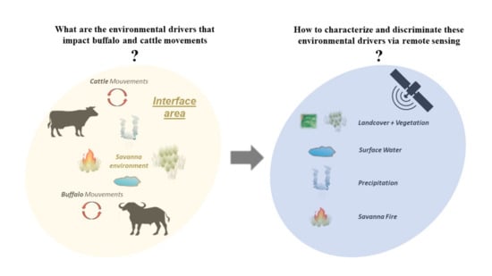
2. Review Article Methodology
3. Environmental Drivers Influencing the Movements of Buffalo and Cattle and the Satellite Remote Sensing Tools to Characterize them
3.1. Landcover
3.1.1. How Landcover and Vegetation Influences Cattle and Buffalo Movements
3.1.2. SRS Basics for Characterizing and Classifying Landcover
3.1.3. SRS for Detecting Landcover and Vegetation Changes
3.1.4. SRS to Characterize Landcover and Vegetation When Studying Animal Movements in Savanna Environments
3.2. Surface Water
3.2.1. How Surface Water Distribution Influences Cattle and Buffalo Movements
3.2.2. SRS Basics for Detecting Water and Water Dynamics
3.2.3. SRS to Detect Surface Water When Studying Animal Movements in Savanna Environments
3.3. Fire Regimes
3.3.1. How Fire Influences Cattle and Buffalo Movements
3.3.2. SRS Basics for Detecting Fire and Fire Dynamics
3.3.3. SRS to Characterize Fire when Studying Animal Movements in Savanna Environments
3.4. Precipitation
3.4.1. How Precipitation Influence Cattle and Buffalo Movements
3.4.2. SRS Basics for Measuring Precipitation
3.4.3. SRS to Measure Precipitation when Studying Animal Movements in Savanna Environments
4. Discussion
4.1. General Observations
4.2. Landcover and Vegetation Characterization
4.3. Surface Water Delineation
4.4. Savanna Fire Characterization
4.5. SRS for Precipitation Characterization
4.6. Selection of Suitable SRS Products to Study Buffalo and Cattle Movements in Southern Africa
5. Conclusions
Supplementary Materials
Author Contributions
Funding
Acknowledgments
Conflicts of Interest
References
- Cleland, J.; Machiyama, K. The Challenges Posed by Demographic Change in sub-Saharan Africa: A Concise Overview: Challenges Posed by Demographic Change in sub-Saharan Africa. Popul. Dev. Rev. 2017, 43, 264–286. [Google Scholar] [CrossRef]
- Wittemyer, G.; Elsen, P.; Bean, W.T.; Burton, A.C.O.; Brashares, J.S. Accelerated Human Population Growth at Protected Area Edges. Science 2008, 321, 123–126. [Google Scholar] [CrossRef] [PubMed]
- Andersson, J.A.; de Garine-Wichatitsky, M.; Cumming, D.H.M.; Dzingirai, V.; Giller, K.E. Transfrontier Conservation Areas: People Living on the Edge, 1st ed.; Routledge: Abingdon, UK, 2017; ISBN 978-1-315-14737-6. [Google Scholar]
- De Garine-Wichatitsky, M.; Caron, A.; Kock, R.; Tschopp, R.; Munyeme, M.; Hofmeyr, M.; Michel, A. A review of bovine tuberculosis at the wildlife–livestock–human interface in sub-Saharan Africa. Epidemiol. Infect. 2013, 141, 1342–1356. [Google Scholar] [CrossRef] [PubMed]
- Bengis, R.G.; Kock, R.A.; Fisher, J.R. Infectious animal diseases: The wildlife/livestock interface: -EN- -FR- -ES-. Rev. Sci. Tech. L’oie 2002, 21, 53–65. [Google Scholar] [CrossRef]
- Chigwenhese, L.; Murwira, A.; Zengeya, F.M.; Masocha, M.; de Garine-Wichatitsky, M.; Caron, A. Monitoring African buffalo (Syncerus caffer) and cattle (Bos taurus) movement across a damaged veterinary control fence at a Southern African wildlife/livestock interface. Afr. J. Ecol. 2016, 54, 415–423. [Google Scholar] [CrossRef]
- Jori, F.; Brahmbhatt, D.; Fosgate, G.T.; Thompson, P.N.; Budke, C.; Ward, M.P.; Ferguson, K.; Gummow, B. A questionnaire-based evaluation of the veterinary cordon fence separating wildlife and livestock along the boundary of the Kruger National Park, South Africa. Prev. Vet. Med. 2011, 100, 210–220. [Google Scholar] [CrossRef]
- Ogutu, J.O.; Owen-Smith, N.; Piepho, H.-P.; Kuloba, B.; Edebe, J. Dynamics of ungulates in relation to climatic and land use changes in an insularized African savanna ecosystem. Biodivers Conserv. 2012, 21, 1033–1053. [Google Scholar] [CrossRef]
- Young, T.P.; Palmer, T.M.; Gadd, M.E. Competition and compensation among cattle, zebras, and elephants in a semi-arid savanna in Laikipia, Kenya. Biol. Conserv. 2005, 122, 351–359. [Google Scholar] [CrossRef]
- Kuiper, T.R.; Loveridge, A.J.; Parker, D.M.; Johnson, P.J.; Hunt, J.E.; Stapelkamp, B.; Sibanda, L.; Macdonald, D.W. Seasonal herding practices influence predation on domestic stock by African lions along a protected area boundary. Biol. Conserv. 2015, 191, 546–554. [Google Scholar] [CrossRef]
- Valls Fox, H. To Drink or Not to Drink? The Influence of Resource Availability on Elephant Foraging and Habitat Selection in a Semi-Arid Savanna. Ph.D. Thesis, Université de Montpellier, Montpellier, France, 2015. [Google Scholar]
- Miguel, E.; Grosbois, V.; Caron, A.; Boulinier, T.; Fritz, H.; Cornélis, D.; Foggin, C.; Makaya, P.V.; Tshabalala, P.T.; de Garine-Wichatitsky, M. Contacts and foot and mouth disease transmission from wild to domestic bovines in Africa. Ecosphere 2013, 4, art51. [Google Scholar] [CrossRef]
- Caron, A.; Miguel, E.; Gomo, C.; Makaya, P.; Pfukenyi, D.M.; Foggin, C.; Hove, T.; de Garine-Wichatitsky, M. Relationship between burden of infection in ungulate populations and wildlife/livestock interfaces. Epidemiol. Infect. 2013, 141, 1522–1535. [Google Scholar] [CrossRef] [PubMed]
- Osofsky, S.A.; Cleaveland, S.; Karesh, W.B.; Kock, M.D.; Nyhus, P.J.; College, C. Conservation and Development Interventions at the Wildlife-Livestock Interface; IUCN—The World Conservation Union: Gland, Switzerland, 2005; p. 242. [Google Scholar]
- Lankester, F.; Davis, A. Pastoralism and wildlife: Historical and current perspectives in the East African rangelands of Kenya and Tanzania. Rev. Sci. Tech. Oie. 2016, 35, 473–484. [Google Scholar] [CrossRef] [PubMed]
- Mascia, M.B.; Pailler, S.; Krithivasan, R.; Roshchanka, V.; Burns, D.; Mlotha, M.J.; Murray, D.R.; Peng, N. Protected area downgrading, downsizing, and degazettement (PADDD) in Africa, Asia, and Latin America and the Caribbean, 1900–2010. Biol. Conserv. 2014, 169, 355–361. [Google Scholar] [CrossRef]
- Ogutu, J.O.; Piepho, H.-P.; Said, M.Y.; Kifugo, S.C. Herbivore Dynamics and Range Contraction in Kajiado County Kenya: Climate and Land Use Changes, Population Pressures, Governance, Policy and Human-wildlife Conflicts. Toecolj 2014, 7, 9–31. [Google Scholar] [CrossRef]
- Mworia, J.K.; Kinyamario, J.I.; Githaiga, J.M. Influence of cultivation, settlements and water sources on wildlife distribution and habitat selection in south-east Kajiado, Kenya. Environ. Conserv. 2008, 35, 117–124. [Google Scholar] [CrossRef]
- Rose, R.A.; Byler, D.; Eastman, J.R.; Fleishman, E.; Geller, G.; Goetz, S.; Guild, L.; Hamilton, H.; Hansen, M.; Headley, R.; et al. Ten ways remote sensing can contribute to conservation. Conserv. Biol. 2015, 29, 350–359. [Google Scholar] [CrossRef]
- Pettorelli, N.; Laurance, W.F.; O’Brien, T.G.; Wegmann, M.; Nagendra, H.; Turner, W. Satellite remote sensing for applied ecologists: Opportunities and challenges. J. Appl. Ecol. 2014, 51, 839–848. [Google Scholar] [CrossRef]
- Zhu, L.; Suomalainen, J.; Liu, J.; Hyyppä, J.; Kaartinen, H.; Haggren, H. A Review: Remote Sensing Sensors. Multi Purp. Appl. Geospat. Data 2017. [Google Scholar] [CrossRef]
- Joshi, N.; Baumann, M.; Ehammer, A.; Fensholt, R.; Grogan, K.; Hostert, P.; Jepsen, M.; Kuemmerle, T.; Meyfroidt, P.; Mitchard, E.; et al. A Review of the Application of Optical and Radar Remote Sensing Data Fusion to Land Use Mapping and Monitoring. Remote Sens. 2016, 8, 70. [Google Scholar] [CrossRef]
- Kaszta, Ż.; Van De Kerchove, R.; Ramoelo, A.; Cho, M.; Madonsela, S.; Mathieu, R.; Wolff, E. Seasonal Separation of African Savanna Components Using Worldview-2 Imagery: A Comparison of Pixel- and Object-Based Approaches and Selected Classification Algorithms. Remote Sens. 2016, 8, 763. [Google Scholar] [CrossRef]
- Marghany, M. Environmental Applications of Remote Sensing; BoD—Books on Demand: Norderstedt, Germany, 2016; ISBN 978-953-51-2443-6. [Google Scholar]
- Pettorelli, N.; Safi, K.; Turner, W. Satellite remote sensing, biodiversity research and conservation of the future. Philos. Trans. R. Soc. B 2014, 369, 20130190. [Google Scholar] [CrossRef] [PubMed]
- Handcock, R.; Swain, D.; Bishop-Hurley, G.; Patison, K.; Wark, T.; Valencia, P.; Corke, P.; O’Neill, C. Monitoring Animal Behaviour and Environmental Interactions Using Wireless Sensor Networks, GPS Collars and Satellite Remote Sensing. Sensors 2009, 9, 3586–3603. [Google Scholar] [CrossRef] [PubMed]
- Hassell, J.M.; Begon, M.; Ward, M.J.; Fèvre, E.M. Urbanization and Disease Emergence: Dynamics at the Wildlife–Livestock–Human Interface. Trends Ecol. Evol. 2017, 32, 55–67. [Google Scholar] [CrossRef]
- Tsalyuk, M.; Kelly, M.; Getz, W.M. Improving the prediction of African savanna vegetation variables using time series of MODIS products. ISPRS J. Photogramm. Remote Sens. 2017, 131, 77–91. [Google Scholar] [CrossRef] [PubMed]
- Naidoo, R.; Preez, P.D.; Stuart-Hill, G.; Chris Weaver, L.; Jago, M.; Wegmann, M. Factors affecting intraspecific variation in home range size of a large African herbivore. Landsc. Ecol. 2012, 27, 1523–1534. [Google Scholar] [CrossRef]
- Mitchard, E.T.A.; Flintrop, C.M. Woody encroachment and forest degradation in sub-Saharan Africa’s woodlands and savannas 1982–2006. Philos. Trans. R. Soc. B Biol. Sci. 2013, 368, 20120406. [Google Scholar] [CrossRef] [PubMed]
- Mathieu, R.; Wessels, K.; Asner, G.; Knapp, D.; van Aardt, J.; Main, R.; Cho, M.; Erasmus, B.; Smit, I. Tree cover, tree height and bare soil cover differences along a land use degradation gradient in semi-arid savannas, South Africa. In Proceedings of the 2009 IEEE International Geoscience and Remote Sensing Symposium, Cape Town, South Africa, 12–17 July 2009; Volume 2, pp. II-194–II-197. [Google Scholar]
- Forkuor, G.; Benewinde Zoungrana, J.-B.; Dimobe, K.; Ouattara, B.; Vadrevu, K.P.; Tondoh, J.E. Above-ground biomass mapping in West African dryland forest using Sentinel-1 and 2 datasets—A case study. Remote Sens. Environ. 2020, 236, 111496. [Google Scholar] [CrossRef]
- Yang, J.; Prince, S.D. Remote sensing of savanna vegetation changes in Eastern Zambia 1972–1989. Int. J. Remote Sens. 2000, 21, 301–322. [Google Scholar] [CrossRef]
- Chuvieco, E. Fundamentals of Satellite Remote Sensing: An Environmental Approach, 2nd ed.; CRC Press: Boca Raton, FL, USA, 2016; ISBN 978-1-4987-2807-2. [Google Scholar]
- Eisfelder, C.; Kuenzer, C.; Dech, S. Derivation of biomass information for semi-arid areas using remote-sensing data. Int. J. Remote Sens. 2012, 33, 2937–2984. [Google Scholar] [CrossRef]
- Pruvot, M.; Musiani, M.; Boyce, M.S.; Kutz, S.; Orsel, K. Integrating livestock management and telemetry data to assess disease transmission risk between wildlife and livestock. Prev. Vet. Med. 2020, 174, 104846. [Google Scholar] [CrossRef]
- Miguel, E.; Grosbois, V.; Fritz, H.; Caron, A.; de Garine-Wichatitsky, M.; Nicod, F.; Loveridge, A.J.; Stapelkamp, B.; Macdonald, D.W.; Valeix, M. Drivers of foot-and-mouth disease in cattle at wild/domestic interface: Insights from farmers, buffalo and lions. Divers. Distrib. 2017, 23, 1018–1030. [Google Scholar] [CrossRef] [PubMed]
- Hebblewhite, M.; Merrill, E.; McDermid, G. A Multi-Scale Test of the Forage Maturation Hypothesis in a Partially Migratory Ungulate Population. Ecol. Monogr. 2008, 78, 141–166. [Google Scholar] [CrossRef]
- Williams, P.H.; Burgess, N.D.; Rahbek, C. Flagship species, ecological complementarity and conserving the diversity of mammals and birds in sub-Saharan Africa. Anim. Conserv. 2000, 3, 249–260. [Google Scholar] [CrossRef]
- Lindsey, P.A.; Roulet, P.A.; Romañach, S.S. Economic and conservation significance of the trophy hunting industry in sub-Saharan Africa. Biol. Conserv. 2007, 134, 455–469. [Google Scholar] [CrossRef]
- Van der Merwe, P.; Saayman, M. Game farms as sustainable ecotourist attractions. Koedoe 2005, 48, 1–10. [Google Scholar] [CrossRef]
- Barnett, R. Food for Thought: The Utilization of Wild Meat in Eastern and Southern Africa; TRAFFIC East-Southern Africa: Nairobi, Kenya, 2000; ISBN 978-9966-9698-0-4. [Google Scholar]
- Eby, S.; Burkepile, D.E.; Fynn, R.W.S.; Burns, C.E.; Govender, N.; Hagenah, N.; Koerner, S.E.; Matchett, K.J.; Thompson, D.I.; Wilcox, K.R.; et al. Loss of a large grazer impacts savanna grassland plant communities similarly in North America and South Africa. Oecologia 2014, 175, 293–303. [Google Scholar] [CrossRef]
- Estes, R.D. The Behavior Guide to African Mammals: Including Hoofed Mammals, Carnivores, Primates; The University of California Press: Berkeley, CA, USA, 2012. [Google Scholar]
- Munag’andu, H.M.; Siamudaala, V.M.; Nambota, A.; Bwalya, J.M.; Munyeme, M.; Mweene, A.S.; Takada, A.; Kida, H. Disease constraints for utilization of the African buffalo (Syncerus caffer) on game ranches in Zambia. Jpn. J. Vet. Sci. 2006, 11, 3–13. [Google Scholar]
- Prins, H. Ecology and Behaviour of the African Buffalo: Social Inequality and Decision Making; Springer Science & Business Media: Berlin, Germany, 1996; ISBN 978-0-412-72520-3. [Google Scholar]
- Ndengu, M.; De Garine-Wichatitsky, M.; Pfukenyi, D.M.; Tivapasi, M.; Mukamuri, B.; Matope, G. Assessment of community awareness and risk perceptions of zoonotic causes of abortion in cattle at three selected livestock–wildlife interface areas of Zimbabwe. Epidemiol. Infect. 2017, 145, 1304–1319. [Google Scholar] [CrossRef]
- Baudron, F.; Andersson, J.A.; Corbeels, M.; Giller, K.E. Failing to Yield? Ploughs, Conservation Agriculture and the Problem of Agricultural Intensification: An Example from the Zambezi Valley, Zimbabwe. J. Dev. Stud. 2012, 48, 393–412. [Google Scholar] [CrossRef]
- Mapiye, C.; Chimonyo, M.; Dzama, K. Seasonal dynamics, production potential and efficiency of cattle in the sweet and sour communal rangelands in South Africa. J. Arid. Environ. 2009. [Google Scholar] [CrossRef]
- Hoffmann, I. Spatial distribution of cattle herds as a response to naturaland social environments: A case study from the Zamfara Reserve, Northwestern Nigeria. Nomadic Peoples 2002, 6, 4–21. [Google Scholar] [CrossRef]
- Augustine, D.J. Response of native ungulates to drought in semi-arid Kenyan rangeland: Ungulate response to drought. Afr. J. Ecol. 2010, 48, 1009–1020. [Google Scholar] [CrossRef]
- Odadi, W.O.; Karachi, M.K.; Abdulrazak, S.A.; Young, T.P. African Wild Ungulates Compete with or Facilitate Cattle Depending on Season. Science 2011, 333, 1753–1755. [Google Scholar] [CrossRef] [PubMed]
- Kaszta, Ż.; Cushman, S.A.; Sillero-Zubiri, C.; Wolff, E.; Marino, J. Where buffalo and cattle meet: Modelling interspecific contact risk using cumulative resistant kernels. Ecography 2018, 41, 1616–1626. [Google Scholar] [CrossRef]
- Zengeya, F.M.; Murwira, A.; Caron, A.; Cornélis, D.; Gandiwa, P.; de Garine-Wichatitsky, M. Spatial overlap between sympatric wild and domestic herbivores links to resource gradients. Remote Sens. Appl. Soc. Environ. 2015, 2, 56–65. [Google Scholar] [CrossRef][Green Version]
- Dougherty, E.R.; Seidel, D.P.; Carlson, C.J.; Getz, W.M. Using Movement Data to Estimate Contact Rates in a Simulated Environmentally-Transmitted Disease System. Ecology 2018. [Google Scholar] [CrossRef]
- Van Schalkwyk, O.L.; Knobel, D.L.; Clercq, E.M.D.; Pus, C.D.; Hendrickx, G.; Van den Bossche, P.V. Description of Events Where African Buffaloes (Syncerus caffer) Strayed from the Endemic Foot-and-Mouth Disease Zone in South Africa, 1998–2008. Transbound. Emerg. Dis. 2016, 63, 333–347. [Google Scholar] [CrossRef]
- Jori, F.; Vosloo, W.; Du Plessis, B.J.A.; Brahmbhatt, D.; Gummow, B.; Thomson, G.R. A qualitative risk assessment of factors contributing to foot and mouth disease outbreaks in cattle along the western boundary of the Kruger National Park. Rev. Sci. Tech. Oie. 2009, 28, 917–931. [Google Scholar] [CrossRef]
- Kock, R.A. The Wildlife Domestic Animal Disease Interface—Should Africa adopt a hard or soft edge? Trans. R. Soc. S. Afr. 2004, 59, 10–14. [Google Scholar] [CrossRef]
- Neumann, W.; Martinuzzi, S.; Estes, A.B.; Pidgeon, A.M.; Dettki, H.; Ericsson, G.; Radeloff, V.C. Opportunities for the application of advanced remotely-sensed data in ecological studies of terrestrial animal movement. Mov. Ecol. 2015, 3, 8. [Google Scholar] [CrossRef]
- Grant, M.J.; Booth, A. A typology of reviews: An analysis of 14 review types and associated methodologies. Health Inf. Libr. J. 2009, 26, 91–108. [Google Scholar] [CrossRef]
- Drusch, M.; Del Bello, U.; Carlier, S.; Colin, O.; Fernandez, V.; Gascon, F.; Hoersch, B.; Isola, C.; Laberinti, P.; Martimort, P.; et al. Sentinel-2: ESA’s Optical High-Resolution Mission for GMES Operational Services. Remote Sens. Environ. 2012, 120, 25–36. [Google Scholar] [CrossRef]
- Tarnavsky, E.; Grimes, D.; Maidment, R.; Black, E.; Allan, R.P.; Stringer, M.; Chadwick, R.; Kayitakire, F. Extension of the TAMSAT Satellite-Based Rainfall Monitoring over Africa and from 1983 to Present. J. Appl. Meteor. Clim. 2014, 53, 2805–2822. [Google Scholar] [CrossRef]
- Maidment, R.I.; Grimes, D.; Allan, R.P.; Tarnavsky, E.; Stringer, M.; Hewison, T.; Roebeling, R.; Black, E. The 30 year TAMSAT African Rainfall Climatology And Time series (TARCAT) data set: 30-YEAR AFRICAN RAINFALL DATASET. J. Geophys. Res. Atmos. 2014, 119, 10,619–10,644. [Google Scholar] [CrossRef]
- Doherty, T.S.; Driscoll, D.A. Coupling movement and landscape ecology for animal conservation in production landscapes. Proc. R. Soc. B Biol. Sci. 2018, 285, 20172272. [Google Scholar] [CrossRef]
- Tyrrell, P.; Russell, S.; Western, D. Seasonal movements of wildlife and livestock in a heterogenous pastoral landscape: Implications for coexistence and community based conservation. Glob. Ecol. Conserv. 2017, 12, 59–72. [Google Scholar] [CrossRef]
- Owen-Smith, N.; Mills, M.G.L. Predator–prey size relationships in an African large-mammal food web. J. Anim. Ecol. 2008, 77, 173–183. [Google Scholar] [CrossRef]
- Odadi, W.O.; Young, T.P.; Okeyo-Owuor, J.B. Effects of Wildlife on Cattle Diets in Laikipia Rangeland, Kenya. Rangel. Ecol. Manag. 2007, 60, 179–185. [Google Scholar] [CrossRef]
- Hibert, F.; Calenge, C.; Fritz, H.; Maillard, D.; Bouché, P.; Ipavec, A.; Convers, A.; Ombredane, D.; de Visscher, M.-N. Spatial avoidance of invading pastoral cattle by wild ungulates: Insights from using point process statistics. Biodivers Conserv. 2010, 19, 2003–2024. [Google Scholar] [CrossRef]
- Hofmann, R.R. Evolutionary steps of ecophysiological adaptation and diversification of ruminants: A comparative view of their digestive system. Oecologia 1989, 78, 443–457. [Google Scholar] [CrossRef]
- Tambling, C.J.; Druce, D.J.; Hayward, M.W.; Castley, J.G.; Adendorff, J.; Kerley, G.I.H. Spatial and temporal changes in group dynamics and range use enable anti-predator responses in African buffalo. Ecology 2012, 93, 1297–1304. [Google Scholar] [CrossRef] [PubMed]
- Furstenburg, D. African Buffalo Syncerus Caffer; Geo Wild Consult (Pty) Ltd.: Gauteng, South Africa, 2010; p. 18. [Google Scholar]
- Tshabalala, T.; Dube, S.; Lent, P.C. Seasonal variation in forages utilized by the African buffalo (Syncerus caffer) in the succulent thicket of South Africa: Seasonal variation in buffalo diet. Afr. J. Ecol. 2009, 48, 438–445. [Google Scholar] [CrossRef]
- Macandza, V.A.; Owen-Smith, N.; Cross, P.C. Forage selection by African buffalo in the late dry season in two landscapes. Afr. J. Wildl. Res. 2004, 34, 9. [Google Scholar]
- Hendricks, H.H.; Clark, B.; Bond, W.J.; Midgley, J.J.; Novellie, P.A. Movement response patterns of livestock to rainfall variability in the Richtersveld National Park. Afr. J. Range Forage Sci. 2005, 22, 117–125. [Google Scholar] [CrossRef]
- Kartzinel, T.R.; Chen, P.A.; Coverdale, T.C.; Erickson, D.L.; Kress, W.J.; Kuzmina, M.L.; Rubenstein, D.I.; Wang, W.; Pringle, R.M. DNA metabarcoding illuminates dietary niche partitioning by African large herbivores. Proc. Natl. Acad. Sci. USA 2015, 112, 8019–8024. [Google Scholar] [CrossRef] [PubMed]
- Prins, H.H.T. Condition Changes and Choice of Social Environment in African Buffalo Bulls. Behaviour 1989, 108, 297–323. [Google Scholar] [CrossRef]
- Stark, M. Daily Movement, Grazing Activity and Diet of Savanna Buffalo, Syncerus-Caffer-Brachyceros, in Benoue-National-Park, Cameroon. Afr. J. Ecol. 1986, 24, 255–262. [Google Scholar] [CrossRef]
- Sianga, K.; Fynn, R.W.S.; Bonyongo, M.C. Seasonal habitat selection by African buffalo Syncerus caffer in the Savuti–Mababe–Linyanti ecosystem of northern Botswana. Koedoe 2017, 59. [Google Scholar] [CrossRef]
- Kaszta, Ż.; Marino, J.; Wolff, E. Fine-scale spatial and seasonal rangeland use by cattle in a foot-and-mouth disease control zones. Agric. Ecosyst. Environ. 2017, 239, 161–172. [Google Scholar] [CrossRef]
- Hansen, M.C.; Potapov, P.V.; Moore, R.; Hancher, M.; Turubanova, S.A.; Tyukavina, A.; Thau, D.; Stehman, S.V.; Goetz, S.J.; Loveland, T.R.; et al. High-Resolution Global Maps of 21st-Century Forest Cover Change. Science 2013, 342, 850–853. [Google Scholar] [CrossRef]
- Mayaux, P.; Bartholomé, E.; Fritz, S.; Belward, A. A new land-cover map of Africa for the year 2000: New land-cover map of Africa. J. Biogeogr. 2004, 31, 861–877. [Google Scholar] [CrossRef]
- Friedl, M.A.; McIver, D.K.; Hodges, J.C.F.; Zhang, X.Y.; Muchoney, D.; Strahler, A.H.; Woodcock, C.E.; Gopal, S.; Schneider, A.; Cooper, A.; et al. Global land cover mapping from MODIS: Algorithms and early results. Remote Sens. Environ. 2002, 83, 287–302. [Google Scholar] [CrossRef]
- Loveland, T.R.; Reed, B.C.; Brown, J.F.; Ohlen, D.O.; Zhu, Z.; Yang, L.; Merchant, J.W. Development of a global land cover characteristics database and IGBP DISCover from 1 km AVHRR data. Int. J. Remote Sens. 2000, 21, 1303–1330. [Google Scholar] [CrossRef]
- Townshend, J.; Justice, C.; Li, W.; Gurney, C.; McManus, J. Global land cover classification by remote sensing: Present capabilities and future possibilities. Remote Sens. Environ. 1991, 35, 243–255. [Google Scholar] [CrossRef]
- Corbane, C.; Lang, S.; Pipkins, K.; Alleaume, S.; Deshayes, M.; García Millán, V.E.; Strasser, T.; Vanden Borre, J.; Toon, S.; Michael, F. Remote sensing for mapping natural habitats and their conservation status—New opportunities and challenges. Int. J. Appl. Earth Obs. Geoinf. 2015, 37, 7–16. [Google Scholar] [CrossRef]
- Pettorelli, N.; Bro-Jørgensen, J.; Durant, S.M.; Blackburn, T.; Carbone, C. Energy Availability and Density Estimates in African Ungulates. Am. Nat. 2009, 173, 698–704. [Google Scholar] [CrossRef]
- Bro-Jørgensen, J.; Brown, M.E.; Pettorelli, N. Using the satellite-derived normalized difference vegetation index (NDVI) to explain ranging patterns in a lek-breeding antelope: The importance of scale. Oecologia 2008, 158, 177–182. [Google Scholar] [CrossRef]
- Cornélis, D.; Benhamou, S.; Janeau, G.; Morellet, N.; Ouedraogo, M.; de Visscher, M.-N. Spatiotemporal dynamics of forage and water resources shape space use of West African savanna buffaloes. J. Mammal. 2011, 92, 1287–1297. [Google Scholar] [CrossRef]
- Zengeya, F.M.; Murwira, A.; Garine-Wichatitsky, M.D. Seasonal habitat selection and space use by a semi-free range herbivore in a heterogeneous savanna landscape. Austral Ecol. 2014, 39, 722–731. [Google Scholar] [CrossRef]
- Valls-Fox, H.; Chamaillé-Jammes, S.; de Garine-Wichatitsky, M.; Perrotton, A.; Courbin, N.; Miguel, E.; Guerbois, C.; Caron, A.; Loveridge, A.; Stapelkamp, B.; et al. Water and cattle shape habitat selection by wild herbivores at the edge of a protected area. Anim. Conserv. 2018, 21, 365–375. [Google Scholar] [CrossRef]
- Naidoo, R.; Brennan, A.; Shapiro, A.C.; Beytell, P.; Aschenborn, O.; Preez, P.D.; Kilian, J.W.; Stuart-Hill, G.; Taylor, R.D. Mapping and assessing the impact of small-scale ephemeral water sources on wildlife in an African seasonal savannah. Ecol. Appl. 2020, e02203. [Google Scholar] [CrossRef]
- Zengeya, F.; Murwira, A.; de Garine-Wichatitsky, M. An IKONOS-based comparison of methods to estimate cattle home ranges in a semi-arid landscape of southern Africa. Int. J. Remote Sens. 2011, 32, 7805–7826. [Google Scholar] [CrossRef]
- Rodriguez-Galiano, V.F.; Ghimire, B.; Rogan, J.; Chica-Olmo, M.; Rigol-Sanchez, J.P. An assessment of the effectiveness of a random forest classifier for land-cover classification. ISPRS J. Photogramm. Remote Sens. 2012, 67, 93–104. [Google Scholar] [CrossRef]
- Breiman, L. Random forests. Mach. Learn. 2001, 45, 5–32. [Google Scholar] [CrossRef]
- Ghimire, B.; Rogan, J.; Miller, J. Contextual land-cover classification: Incorporating spatial dependence in land-cover classification models using random forests and the Getis statistic. Remote Sens. Lett. 2010, 1, 45–54. [Google Scholar] [CrossRef]
- Chan, J.C.-W.; Paelinckx, D. Evaluation of Random Forest and Adaboost tree-based ensemble classification and spectral band selection for ecotope mapping using airborne hyperspectral imagery. Remote Sens. Environ. 2008, 112, 2999–3011. [Google Scholar] [CrossRef]
- Du, P.; Samat, A.; Waske, B.; Liu, S.; Li, Z. Random Forest and Rotation Forest for fully polarized SAR image classification using polarimetric and spatial features. ISPRS J. Photogramm. Remote Sens. 2015, 105, 38–53. [Google Scholar] [CrossRef]
- Gislason, P.O.; Benediktsson, J.A.; Sveinsson, J.R. Random Forests for land cover classification. Pattern Recognit. Lett. 2006, 27, 294–300. [Google Scholar] [CrossRef]
- Duda, T.; Canty, M. Unsupervised classification of satellite imagery: Choosing a good algorithm. Int. J. Remote Sens. 2002, 23, 2193–2212. [Google Scholar] [CrossRef]
- Blaschke, T.; Hay, G.J.; Kelly, M.; Lang, S.; Hofmann, P.; Addink, E.; Queiroz Feitosa, R.; van der Meer, F.; van der Werff, H.; van Coillie, F.; et al. Geographic Object-Based Image Analysis—Towards a new paradigm. ISPRS J. Photogramm. Remote Sens. 2014, 87, 180–191. [Google Scholar] [CrossRef]
- Xu, Y.; Yu, L.; Feng, D.; Peng, D.; Li, C.; Huang, X.; Lu, H.; Gong, P. Comparisons of three recent moderate resolution African land cover datasets: CGLS-LC100, ESA-S2-LC20, and FROM-GLC-Africa30. Int. J. Remote Sens. 2019, 40, 6185–6202. [Google Scholar] [CrossRef]
- Arraut, E.M.; Loveridge, A.J.; Chamaillé-Jammes, S.; Valls-Fox, H.; Macdonald, D.W. The 2013–2014 vegetation structure map of Hwange National Park, Zimbabwe, produced using free satellite images and software. Koedoe Afr. Prot. Area Conserv. Sci. 2018, 60. [Google Scholar] [CrossRef]
- Liu, B.; Chen, J.; Chen, J.; Zhang, W. Land Cover Change Detection Using Multiple Shape Parameters of Spectral and NDVI Curves. Remote Sens. 2018, 10, 1251. [Google Scholar] [CrossRef]
- Münch, Z.; Gibson, L.; Palmer, A. Monitoring Effects of Land Cover Change on Biophysical Drivers in Rangelands Using Albedo. Land 2019, 8, 33. [Google Scholar] [CrossRef]
- Gómez, C.; White, J.C.; Wulder, M.A. Optical remotely sensed time series data for land cover classification: A review. ISPRS J. Photogramm. Remote Sens. 2016, 116, 55–72. [Google Scholar] [CrossRef]
- Balzter, H.; Cole, B.; Thiel, C.; Schmullius, C. Mapping CORINE Land Cover from Sentinel-1A SAR and SRTM Digital Elevation Model Data using Random Forests. Remote Sens. 2015, 7, 14876–14898. [Google Scholar] [CrossRef]
- Longepe, N.; Rakwatin, P.; Isoguchi, O.; Shimada, M.; Uryu, Y.; Yulianto, K. Assessment of ALOS PALSAR 50 m Orthorectified FBD Data for Regional Land Cover Classification by Support Vector Machines. IEEE Trans. Geosci. Remote Sens. 2011, 49, 2135–2150. [Google Scholar] [CrossRef]
- Abdikan, S.; Sanli, F.B.; Ustuner, M.; Calò, F. Land Cover Mapping Using Sentinel-1 SAR Data. Int. Arch. Photogramm. Remote Sens. Spat. Inf. Sci. 2016, XLI-B7, 757–761. [Google Scholar] [CrossRef]
- Reiche, J.; Verhoeven, R.; Verbesselt, J.; Hamunyela, E.; Wielaard, N.; Herold, M. Characterizing Tropical Forest Cover Loss Using Dense Sentinel-1 Data and Active Fire Alerts. Remote Sens. 2018, 10, 777. [Google Scholar] [CrossRef]
- Bouvet, A.; Mermoz, S.; Le Toan, T.; Villard, L.; Mathieu, R.; Naidoo, L.; Asner, G.P. An above-ground biomass map of African savannahs and woodlands at 25m resolution derived from ALOS PALSAR. Remote Sens. Environ. 2018, 206, 156–173. [Google Scholar] [CrossRef]
- De Alban, J.D.T.; Connette, G.M.; Oswald, P.; Webb, E.L. Combined Landsat and L-Band SAR Data Improves Land Cover Classification and Change Detection in Dynamic Tropical Landscapes. Remote Sens. 2018, 10, 306. [Google Scholar] [CrossRef]
- Mercier, A.; Betbeder, J.; Rumiano, F.; Gond, V.; Bourgoin, C.; Cornu, G.; Blanc, L.; Baudry, J.; Huber-Moy, L. Evaluation of the joint use of Sentinel-1 & 2 time series for land cover classification of large areas: From temperate to tropical landscapes. Remoste Sens. 2018, 11, 979. [Google Scholar] [CrossRef]
- Reiche, J.; Lucas, R.; Mitchell, A.L.; Verbesselt, J.; Hoekman, D.H.; Haarpaintner, J.; Kellndorfer, J.M.; Rosenqvist, A.; Lehmann, E.A.; Woodcock, C.E.; et al. Combining satellite data for better tropical forest monitoring. Nat. Clim. Chang. 2016, 6, 120–122. [Google Scholar] [CrossRef]
- Li, W.; MacBean, N.; Ciais, P.; Defourny, P.; Lamarche, C.; Bontemps, S.; Houghton, R.A.; Peng, S. Gross and net land cover changes in the main plant functional types derived from the annual ESA CCI land cover maps (1992–2015). Earth Syst. Sci. Data 2018, 10, 219–234. [Google Scholar] [CrossRef]
- Friedl, M.A.; Sulla-Menashe, D.; Tan, B.; Schneider, A.; Ramankutty, N.; Sibley, A.; Huang, X. MODIS Collection 5 global land cover: Algorithm refinements and characterization of new datasets. Remote Sens. Environ. 2010, 114, 168–182. [Google Scholar] [CrossRef]
- Chen, J.; Chen, J.; Liao, A.; Cao, X.; Chen, L.; Chen, X.; He, C.; Han, G.; Peng, S.; Lu, M.; et al. Global land cover mapping at 30m resolution: A POK-based operational approach. Isprs J. Photogramm. Remote Sens. 2015, 103, 7–27. [Google Scholar] [CrossRef]
- Bartholomé, E.; Belward, A.S. GLC2000: A new approach to global land cover mapping from Earth observation data. Int. J. Remote Sens. 2005, 26, 1959–1977. [Google Scholar] [CrossRef]
- Arino, O.; Ramos Perez, J.J.; Kalogirou, V.; Bontemps, S.; Defourny, P.; Van Bogaert, E. Global Land Cover Map for 2009 (GlobCover 2009); © European Space Agency (ESA) & Université catholique de Louvain (UCL), PANGAEA: Paris, France; Louvain, Belgium, 2012. [Google Scholar] [CrossRef]
- Tateishi, R.; Uriyangqai, B.; Al-Bilbisi, H.; Ghar, M.A.; Tsend-Ayush, J.; Kobayashi, T.; Kasimu, A.; Hoan, N.T.; Shalaby, A.; Alsaaideh, B.; et al. Production of global land cover data—GLCNMO. Int. J. Digit. Earth 2011, 4, 22–49. [Google Scholar] [CrossRef]
- Latham, J.S.; Cumani, R. Global Land Cover SHARE (GLC-SHARE) Database Beta-Release Version 1.0. 2014. Available online: http://www.fao.org/uploads/media/glc-share-doc.pdf (accessed on 3 July 2020).
- Wang, J.; Zhao, Y.; Li, C.; Yu, L.; Liu, D.; Gong, P. Mapping global land cover in 2001 and 2010 with spatial-temporal consistency at 250 m resolution. ISPRS J. Photogramm. Remote Sens. 2015, 103, 38–47. [Google Scholar] [CrossRef]
- Gong, P.; Wang, J.; Yu, L.; Zhao, Y.; Zhao, Y.; Liang, L.; Niu, Z.; Huang, X.; Fu, H.; Liu, S.; et al. Finer resolution observation and monitoring of global land cover: First mapping results with Landsat TM and ETM+ data. Int. J. Remote Sens. 2013, 34, 2607–2654. [Google Scholar] [CrossRef]
- Sexton, J.O.; Song, X.-P.; Feng, M.; Noojipady, P.; Anand, A.; Huang, C.; Kim, D.-H.; Collins, K.M.; Channan, S.; DiMiceli, C.; et al. Global, 30-m resolution continuous fields of tree cover: Landsat-based rescaling of MODIS vegetation continuous fields with lidar-based estimates of error. Int. J. Digit. Earth 2013, 6, 427–448. [Google Scholar] [CrossRef]
- Buchhorn, M.; Bertels, L.; Smets, B.; Lesiv, M.; Wur, N.E.T. Copernicus Global Land Operations “Vegetation and Energy”. 2017. Available online: https://land.copernicus.eu/global/sites/cgls.vito.be/files/products/CGLOPS1_PUM_LC100m-V1_I1.00.pdf (accessed on 3 July 2020).
- Lesiv, M.; Fritz, S.; McCallum, I.; Tsendbazar, N.; Herold, M.; Pekel, J.-F.; Buchhorn, M.; Smets, B.; Van De Kerchove, R. Evaluation of ESA CCI Prototype Land Cover Map at 20 m. 2017. Available online: http://pure.iiasa.ac.at/id/eprint/14979/ (accessed on 3 July 2020).
- Jianya, G.; Haigang, S.; Guorui, M.; Qiming, Z. A Review of multi-temporal remote sensing data change detection algorithms. Remote Sens. 2008, 5, 7. [Google Scholar]
- Vanderpost, C.; Ringrose, S.; Matheson, W.; Arntzen, J. Satellite based long-term assessment of rangeland condition in semi-arid areas: An example from Botswana. J. Arid Environ. 2011, 75, 383–389. [Google Scholar] [CrossRef]
- Kindu, M.; Schneider, T.; Teketay, D.; Knoke, T. Land Use/Land Cover Change Analysis Using Object-Based Classification Approach in Munessa-Shashemene Landscape of the Ethiopian Highlands. Remote Sens. 2013, 5, 2411–2435. [Google Scholar] [CrossRef]
- Kerr, J.T.; Ostrovsky, M. From space to species: Ecological applications for remote sensing. Trends Ecol. Evol. 2003, 18, 299–305. [Google Scholar] [CrossRef]
- Turner, W.; Spector, S.; Gardiner, N.; Fladeland, M.; Sterling, E.; Steininger, M. Remote sensing for biodiversity science and conservation. Trends Ecol. Evol. 2003, 18, 306–314. [Google Scholar] [CrossRef]
- Pettorelli, N.; Vik, J.O.; Mysterud, A.; Gaillard, J.-M.; Tucker, C.J.; Stenseth, N.C. Using the satellite-derived NDVI to assess ecological responses to environmental change. Trends Ecol. Evol. 2005, 20, 503–510. [Google Scholar] [CrossRef]
- Wang, Q.; Adiku, S.; Tenhunen, J.; Granier, A. On the relationship of NDVI with leaf area index in a deciduous forest site. Remote Sens. Environ. 2005, 94, 244–255. [Google Scholar] [CrossRef]
- Buermann, W. Analysis of a multiyear global vegetation leaf area index data set. J. Geophys. Res. 2002, 107, 4646. [Google Scholar] [CrossRef]
- Myneni, R.B.; Hall, F.G.; Sellers, P.J.; Marshak, A.L. The interpretation of spectral vegetation indexes. IEEE Trans. Geosci. Remote Sens. 1995, 33, 481–486. [Google Scholar] [CrossRef]
- Ryan, S.J.; Cross, P.C.; Winnie, J.; Hay, C.; Bowers, J.; Getz, W.M. The utility of normalized difference vegetation index for predicting African buffalo forage quality. J. Wildl. Manag. 2012, 76, 1499–1508. [Google Scholar] [CrossRef]
- Hamel, S.; Garel, M.; Festa-Bianchet, M.; Gaillard, J.-M.; Côté, S.D. Spring Normalized Difference Vegetation Index (NDVI) predicts annual variation in timing of peak faecal crude protein in mountain ungulates. J. Appl. Ecol. 2009, 46, 582–589. [Google Scholar] [CrossRef]
- Pettorelli, N.; Pelletier, F.; von Hardenberg, A.; Festa-Bianchet, M.; Côté, S.D. Early Onset of Vegetation Growth Vs. Rapid Green-up: Impacts on Juvenile Mountain Ungulates. Ecology 2007, 88, 381–390. [Google Scholar] [CrossRef] [PubMed]
- MØller, A.P.; Merilä, J. Analysis and Interpretation of Long-Term Studies Investigating Responses to Climate Change. In Advances in Ecological Research; Birds and Climate Change; Academic Press: Cambridge, MA, USA, 2004; Volume 35, pp. 111–130. [Google Scholar]
- Andersen, R.; Herfindel, I.; Sæther, B.-E.; Linnell, J.D.C.; Oddén, J.; Liberg, O. When range expansion rate is faster in marginal habitats. Oikos 2004, 107, 210–214. [Google Scholar] [CrossRef]
- Guan, K.; Wood, E.F.; Medvigy, D.; Kimball, J.; Pan, M.; Caylor, K.K.; Sheffield, J.; Xu, X.; Jones, M.O. Terrestrial hydrological controls on land surface phenology of African savannas and woodlands: Hydrology controls on African phenology. J. Geophys. Res. Biogeosci. 2014, 119, 1652–1669. [Google Scholar] [CrossRef]
- Archibald, S.; Hempson, G.P. Competing consumers: Contrasting the patterns and impacts of fire and mammalian herbivory in Africa. Phil. Trans. R. Soc. B 2016, 371, 20150309. [Google Scholar] [CrossRef]
- Pinty, B.; Verstraete, M.M. GEMI: A non-linear index to monitor global vegetation from satellites. Vegetation 1992, 101, 15–20. [Google Scholar] [CrossRef]
- Huete, A.R. A soil-adjusted vegetation index (SAVI). Remote Sens. Environ. 1988, 25, 295–309. [Google Scholar] [CrossRef]
- Tsalyuk, M.; Kilian, W.; Reineking, B.; Getz, W.M. Temporal variation in resource selection of African elephants follows long-term variability in resource availability. Ecol. Monogr. 2019, 89, e01348. [Google Scholar] [CrossRef]
- Boone, R.B.; Thirgood, S.J.; Hopcraft, J.G.C. Serengeti Wildebeest Migratory Patterns Modeled from Rainfall and New Vegetation Growth. Available online: https://esajournals.onlinelibrary.wiley.com/doi/abs/10.1890/00129658%282006%2987%5B1987%3ASWMPMF%5D2.0.CO%3B2 (accessed on 13 August 2019).
- Naidoo, R.; Du Preez, P.; Stuart-Hill, G.; Jago, M.; Wegmann, M. Home on the Range: Factors Explaining Partial Migration of African Buffalo in a Tropical Environment. PLoS ONE 2012, 7, e36527. [Google Scholar] [CrossRef]
- Sitters, J.; Heitkönig, I.M.A.; Holmgren, M.; Ojwang’, G.S.O. Herded cattle and wild grazers partition water but share forage resources during dry years in East African savannas. Biol. Conserv. 2009, 142, 738–750. [Google Scholar] [CrossRef]
- Huete, A.R.; Liu, H.Q.; Batchily, K.; Leeuwen, W. van A comparison of vegetation indices over a global set of TM images for EOS-MODIS. Remote Sens. Environ. 1997, 59, 440–451. [Google Scholar] [CrossRef]
- Rouse, W.; Haas, R.H. Monitoring vegetation systems in the Great Plains with ERTS. Proc. Third Earth Resour. Technol. Satell. 1 Symp. 1974, 9, 301–317. [Google Scholar]
- Huete, A.; Didan, K.; Miura, T.; Rodriguez, E.P.; Gao, X.; Ferreira, L.G. Overview of the radiometric and biophysical performance of the MODIS vegetation indices. Remote Sens. Environ. 2002, 83, 195–213. [Google Scholar] [CrossRef]
- Qi, J.; Chehbouni, A.; Huete, A.R.; Kerr, Y.H.; Sorooshian, S. A modified soil adjusted vegetation index. Remote Sens. Environ. 1994, 48, 119–126. [Google Scholar] [CrossRef]
- Richardson, A.J.; Wiegand, C.L. Distinguishing Vegetation from Soil Background Information. Photogramm. Eng. Remote Sens. 1977, 43, 1541–1552. [Google Scholar]
- Haboudane, D. Hyperspectral vegetation indices and novel algorithms for predicting green LAI of crop canopies: Modeling and validation in the context of precision agriculture. Remote Sens. Environ. 2004, 90, 337–352. [Google Scholar] [CrossRef]
- Baret, F.; Jacquemoud, S.; Hanocq, J.F. About the soil line concept in remote sensing. Adv. Space Res. 1993, 13, 281–284. [Google Scholar] [CrossRef]
- Batten, G.D. Plant analysis using near infrared reflectance spectroscopy: The potential and the limitations. Aust. J. Exp. Agric. 1998, 38, 697–706. [Google Scholar] [CrossRef]
- Jiang, Z.; Huete, A.; Didan, K.; Miura, T. Development of a two-band enhanced vegetation index without a blue band. Remote Sens. Environ. 2008, 112, 3833–3845. [Google Scholar] [CrossRef]
- Daughtry, C. Estimating Corn Leaf Chlorophyll Concentration from Leaf and Canopy Reflectance. Remote Sens. Environ. 2000, 74, 229–239. [Google Scholar] [CrossRef]
- OwenSmith, N. Ecological guidelines for waterpoints in extensive protected areas. S. Afr. J. Wildl. Res. 1996, 26, 107–112. [Google Scholar]
- Smit, I.P.J.; Grant, C.C.; Devereux, B.J. Do artificial waterholes influence the way herbivores use the landscape? Herbivore distribution patterns around rivers and artificial surface water sources in a large African savanna park. Biol. Conserv. 2007, 136, 85–99. [Google Scholar] [CrossRef]
- Ryan, S.J.; Knechtel, C.U.; Getz, W.M. Range and Habitat Selection of African Buffalo in South Africa. J. Wildl. Manag. 2006, 70, 764–776. [Google Scholar] [CrossRef]
- Hunter, C.G. Land uses on the Botswana/Zimbabwe border and their effects on buffalo. S. Afr. J. Wildl. Res. 1996, 26, 136–150. [Google Scholar]
- Western, D. Water availability and its influence on the structure and dynamics of a savannah large mammal community. Afr. J. Ecol. 1975, 13, 265–286. [Google Scholar] [CrossRef]
- Cornélis, D.; Melletti, M.; Korte, L.; Ryan, S.J.; Mirabile, M.; Prin, T.; Prins, H. African Buffalo (Syncerus Caffer Sparrman, 1779). Available online: http://agritrop.cirad.fr/578582/ (accessed on 28 July 2020).
- Moyo, B.; Dube, S.; Lesoli, M.; Masika, P. Seasonal habitat use and movement patterns of cattle grazing different rangeland types in the communal areas of the Eastern Cape, South Africa. Afr. J. Agric. Res. 2013, 8, 36–45. [Google Scholar] [CrossRef]
- Scoones, I. Exploiting heterogeneity:habitat use by cattle in dryland Zimbabwe. J. Arid Environ. 1995, 29, 221–237. [Google Scholar] [CrossRef]
- Bennitt, E.; Bonyongo, M.C.; Harris, S. Habitat Selection by African Buffalo (Syncerus caffer) in Response to Landscape-Level Fluctuations in Water Availability on Two Temporal Scales. PLoS ONE 2014, 9, e101346. [Google Scholar] [CrossRef]
- Redfern, J.V.; Grant, R.; Biggs, H.; Getz, W.M. Surface water constraints on herbivore foraging in the Kruger National Park, South Africa. Ecology 2003, 84, 2092–2107. [Google Scholar] [CrossRef]
- Traill, L.W.; Bigalke, R.C. A presence-only habitat suitability model for large grazing African ungulates and its utility for wildlife management. Afr. J. Ecol. 2007, 45, 347–354. [Google Scholar] [CrossRef]
- Fritz, H.; Garine-Wichatitsky, M.D.; Letessier, G. Habitat Use by Sympatric Wild and Domestic Herbivores in an African Savanna Woodland: The Influence of Cattle Spatial Behaviour. J. Appl. Ecol. 1996, 33, 589. [Google Scholar] [CrossRef]
- Georgiadis, N.J.; Ihwagi, F.; Olwero, J.G.N.; Romañach, S.S. Savanna herbivore dynamics in a livestock-dominated landscape. II: Ecological, conservation, and management implications of predator restoration. Biol. Conserv. 2007, 137, 473–483. [Google Scholar] [CrossRef]
- Huang, C.; Chen, Y.; Zhang, S.; Wu, J. Detecting, Extracting, and Monitoring Surface Water From Space Using Optical Sensors: A Review. Rev. Geophys. 2018, 56, 333–360. [Google Scholar] [CrossRef]
- Majozi, N.P.; Mannaerts, C.M.; Ramoelo, A.; Mathieu, R.; Nickless, A.; Verhoef, W. Analysing surface energy balance closure and partitioning over a semi-arid savanna FLUXNET site in Skukuza, Kruger National Park, South Africa. Hydrol. Earth Syst. Sci. 2017, 21, 3401–3415. [Google Scholar] [CrossRef]
- Donchyts, G.; Baart, F.; Winsemius, H.; Gorelick, N.; Kwadijk, J.; van de Giesen, N. Earth’s surface water change over the past 30 years. Nat. Clim. Chang. 2016, 6, 810. [Google Scholar] [CrossRef]
- Huang, C.; Chen, Y.; Wu, J.; Li, L.; Liu, R. An evaluation of Suomi NPP-VIIRS data for surface water detection. Remote Sens. Lett. 2015, 6, 155–164. [Google Scholar] [CrossRef]
- Ramoelo, A.; Majozi, N.; Mathieu, R.; Jovanovic, N.; Nickless, A.; Dzikiti, S. Validation of Global Evapotranspiration Product (MOD16) using Flux Tower Data in the African Savanna, South Africa. Remote Sens. 2014, 6, 7406–7423. [Google Scholar] [CrossRef]
- Alsdorf, D.E.; Rodríguez, E.; Lettenmaier, D.P. Measuring surface water from space. Rev. Geophys. 2007, 45. [Google Scholar] [CrossRef]
- Soti, V.; Puech, C.; Lo Seen, D.; Bertran, A.; Vignolles, C.; Mondet, B.; Dessay, N.; Tran, A. The potential for remote sensing and hydrologic modelling to assess the spatio-temporal dynamics of ponds in the Ferlo Region (Senegal). Hydrol. Earth Syst. Sci. 2010, 14, 1449–1464. [Google Scholar] [CrossRef]
- Acharya, T.; Lee, D.; Yang, I.; Lee, J. Identification of Water Bodies in a Landsat 8 OLI Image Using a J48 Decision Tree. Sensors 2016, 16, 1075. [Google Scholar] [CrossRef]
- Sun, D.; Yu, Y.; Goldberg, M.D. Deriving Water Fraction and Flood Maps From MODIS Images Using a Decision Tree Approach. IEEE J. Sel. Top. Appl. Earth Obs. Remote Sens. 2011, 4, 814–825. [Google Scholar] [CrossRef]
- Frazier, P.S.; Page, K.J. Water Body Detection and Delineation with Landsat TM Data. Photogramm. Eng. Remote Sens. 2000, 12, 1461–1467. [Google Scholar]
- Mohammadi, A.; Costelloe, J.F.; Ryu, D. Application of time series of remotely sensed normalized difference water, vegetation and moisture indices in characterizing flood dynamics of large-scale arid zone floodplains. Remote Sens. Environ. 2017, 190, 70–82. [Google Scholar] [CrossRef]
- Chen, Y.; Wang, B.; Pollino, C.A.; Cuddy, S.M.; Merrin, L.E.; Huang, C. Estimate of flood inundation and retention on wetlands using remote sensing and GIS: Spatial modeliing of flood inundation and retention on wetlands. Ecohydrology 2014. [Google Scholar] [CrossRef]
- Huang, C.; Chen, Y.; Wu, J. DEM-based modification of pixel-swapping algorithm for enhancing floodplain inundation mapping. Int. J. Remote Sens. 2014, 35, 365–381. [Google Scholar] [CrossRef]
- Owen, H.J.F.; Duncan, C.; Pettorelli, N. Testing the water: Detecting artificial water points using freely available satellite data and open source software. Remote Sens. Ecol. Conserv. 2015, 1, 61–72. [Google Scholar] [CrossRef]
- Hardisky, M.; Klemas, V.; Smart, R. The Influence of Soil-Salinity, Growth Form, and Leaf Moisture on the Spectral Radiance of Spartina-Alterniflora Canopies. Photogramm. Eng. Remote Sens. 1983, 49, 77–83. [Google Scholar]
- McFeeters, S.K. The use of the Normalized Difference Water Index (NDWI) in the delineation of open water features. Int. J. Remote Sens. 1996, 17, 1425–1432. [Google Scholar] [CrossRef]
- Gao, B. NDWI—A normalized difference water index for remote sensing of vegetation liquid water from space. Remote Sens. Environ. 1996, 58, 257–266. [Google Scholar] [CrossRef]
- Lacaux, J.P.; Tourre, Y.M.; Vignolles, C.; Ndione, J.A.; Lafaye, M. Classification of ponds from high-spatial resolution remote sensing: Application to Rift Valley Fever epidemics in Senegal. Remote Sens. Environ. 2007, 106, 66–74. [Google Scholar] [CrossRef]
- Clandillon, S.; Fraipont, P.; Yesou, H. Assessment of the future SPOT 4 MIR for wetland monitoring and soil moisture analysis: Simulation over the Ried Center Alsace (France). In Proceedings of the Remote Sensing for Agriculture, Forestry, and Natural Resources, International Society for Optics and Photonics, Paris, France, 1 January 1995; Volume 2585, pp. 102–111. [Google Scholar]
- Feyisa, G.L.; Meilby, H.; Fensholt, R.; Proud, S.R. Automated Water Extraction Index: A new technique for surface water mapping using Landsat imagery. Remote Sens. Environ. 2014, 140, 23–35. [Google Scholar] [CrossRef]
- Fisher, A.; Flood, N.; Danaher, T. Comparing Landsat water index methods for automated water classification in eastern Australia. Remote Sens. Environ. 2016, 175, 167–182. [Google Scholar] [CrossRef]
- Jin, H.; Huang, C.; Lang, M.W.; Yeo, I.-Y.; Stehman, S.V. Monitoring of wetland inundation dynamics in the Delmarva Peninsula using Landsat time-series imagery from 1985 to 2011. Remote Sens. Environ. 2017, 190, 26–41. [Google Scholar] [CrossRef]
- Bioresita, F.; Puissant, A.; Stumpf, A.; Malet, J.-P. A Method for Automatic and Rapid Mapping of Water Surfaces from Sentinel-1 Imagery. Remote Sens. 2018, 10, 217. [Google Scholar] [CrossRef]
- Chapman, B.; McDonald, K.; Shimada, M.; Rosenqvist, A.; Schroeder, R.; Hess, L. Mapping Regional Inundation with Spaceborne L-Band SAR. Remote Sens. 2015, 7, 5440–5470. [Google Scholar] [CrossRef]
- Martinis, S.; Twele, A.; Voigt, S. Unsupervised Extraction of Flood-Induced Backscatter Changes in SAR Data Using Markov Image Modeling on Irregular Graphs. IEEE Trans. Geosci. Remote Sens. 2011, 49, 251–263. [Google Scholar] [CrossRef]
- Bartsch, A.; Trofaier, A.M.; Hayman, G.; Sabel, D.; Schlaffer, S.; Clark, D.B.; Blyth, E. Detection of open water dynamics with ENVISAT ASAR in support of land surface modelling at high latitudes. Biogeosciences 2012, 9, 703–714. [Google Scholar] [CrossRef]
- Martinis, S.; Twele, A.; Voigt, S. Towards operational near real-time flood detection using a split-based automatic thresholding procedure on high resolution TerraSAR-X data. Nat. Hazards Earth Syst. Sci. 2009, 9, 303–314. [Google Scholar] [CrossRef]
- Simon, R.N.; Tormos, T.; Danis, P.A. Geographic Object Based Image Analysis Using very High Spatial and Temporal Resolution Radar and Optical Imagery in Tracking Water Level Fluctuations in a Freshwater Reservoir. South-Eastern Eur. J. Earth Obs. Geomat. 2014, 3, 287–291. [Google Scholar]
- Evans, T.L.; Costa, M.; Silva, T.S.F.; Telmer, K. Using PALSAR and RADARSAT-2 to map land cover andinundation in the Brazilian Pantanal. In Proceedings of the 3e Simpósio de Geotecnologias no Pantanal, Caceres, Brazil, 16–20 October 2010; pp. 485–494. [Google Scholar]
- Mitchell, A.L.; Milne, A.K.; Tapley, I. Towards an operational SAR monitoring system for monitoring environmental flows in the Macquarie Marshes. Wetl. Ecol. Manag. 2015, 23, 61–77. [Google Scholar] [CrossRef]
- Martinez, J.; Letoan, T. Mapping of flood dynamics and spatial distribution of vegetation in the Amazon floodplain using multitemporal SAR data. Remote Sens. Environ. 2007, 108, 209–223. [Google Scholar] [CrossRef]
- Twele, A.; Cao, W.; Plank, S.; Martinis, S. Sentinel-1-based flood mapping: A fully automated processing chain. Int. J. Remote Sens. 2016, 37, 2990–3004. [Google Scholar] [CrossRef]
- Martinis, S.; Kuenzer, C.; Wendleder, A.; Huth, J.; Twele, A.; Roth, A.; Dech, S. Comparing four operational SAR-based water and flood detection approaches. Int. J. Remote Sens. 2015, 36, 3519–3543. [Google Scholar] [CrossRef]
- Westerhoff, R.S.; Kleuskens, M.P.H.; Winsemius, H.C.; Huizinga, H.J.; Brakenridge, G.R.; Bishop, C. Automated global water mapping based on wide-swath orbital synthetic-aperture radar. Hydrol. Earth Syst. Sci. 2013, 17, 651–663. [Google Scholar] [CrossRef]
- Brisco, B.; Short, N. A semi-automated tool for surface water mapping with RADARSAT-. Can. J. Remote Sens. 2009, 35, 9. [Google Scholar]
- Schumann, G.; Bates, P.D.; Horritt, M.S.; Matgen, P.; Pappenberger, F. Progress in integration of remote sensing–derived flood extent and stage data and hydraulic models. Rev. Geophys. 2009, 47, RG4001. [Google Scholar] [CrossRef]
- Bertram, A.; Wendleder, A.; Schmitt, A.; Huber, M. Long-term monitoring of water dynamics in the Sahel region using the Multi-SAR-System. ISPRS Int. Arch. Photogramm. Remote Sens. Spat. Inf. Sci. 2016, XLI-B8, 313–320. [Google Scholar] [CrossRef]
- Haas, E.M.; Bartholomé, E.; Lambin, E.F.; Vanacker, V. Remotely sensed surface water extent as an indicator of short-term changes in ecohydrological processes in sub-Saharan Western Africa. Remote Sens. Environ. 2011, 115, 3436–3445. [Google Scholar] [CrossRef]
- Moser, L.; Voigt, S.; Schoepfer, E.; Palmer, S. Multitemporal Wetland Monitoring in Sub-Saharan West-Africa Using Medium Resolution Optical Satellite Data. IEEE J. Sel. Top. Appl. Earth Obs. Remote Sens. 2014, 7, 3402–3415. [Google Scholar] [CrossRef]
- Rokni, K.; Ahmad, A.; Solaimani, K.; Hazini, S. A new approach for surface water change detection: Integration of pixel level image fusion and image classification techniques. Int. J. Appl. Earth Obs. Geoinf. 2015, 34, 226–234. [Google Scholar] [CrossRef]
- Du, Y.; Zhang, Y.; Ling, F.; Wang, Q.; Li, W.; Li, X. Water Bodies’ Mapping from Sentinel-2 Imagery with Modified Normalized Difference Water Index at 10-m Spatial Resolution Produced by Sharpening the SWIR Band. Remote Sens. 2016, 8, 354. [Google Scholar] [CrossRef]
- Dzinotizei, Z.; Murwira, A.; Zengeya, F.M.; Guerrini, L. Mapping waterholes and testing for aridity using a remote sensing water index in a southern African semi-arid wildlife area. Geocarto Int. 2018, 33, 1268–1280. [Google Scholar] [CrossRef]
- Zvidzai, M.; Murwira, A.; Caron, A. Waterhole use patterns at the wildlife/livestock interface in a semi-arid savanna of Southern Africa. Int. J. Dev. Sustain. 2013, 17, 455–471. [Google Scholar]
- Crosmary, W.-G.; Valeix, M.; Fritz, H.; Madzikanda, H.; Côté, S.D. African ungulates and their drinking problems: Hunting and predation risks constrain access to water. Anim. Behav. 2012, 83, 145–153. [Google Scholar] [CrossRef]
- Chamaillé-Jammes, S.; Fritz, H.; Murindagomo, F. Climate-driven fluctuations in surface-water availability and the buffering role of artificial pumping in an African savanna: Potential implication for herbivore dynamics. Austral Ecol. 2007, 32, 740–748. [Google Scholar] [CrossRef]
- Chamaillé-Jammes, S.; Charbonnel, A.; Dray, S.; Madzikanda, H.; Fritz, H. Spatial Distribution of a Large Herbivore Community at Waterholes: An Assessment of Its Stability over Years in Hwange National Park, Zimbabwe. PLoS ONE 2016, 11, e0153639. [Google Scholar] [CrossRef]
- Pekel, J.-F.; Cottam, A.; Gorelick, N.; Belward, A.S. High-resolution mapping of global surface water and its long-term changes. Nature 2016, 540, 418–422. [Google Scholar] [CrossRef]
- Lamarche, C.; Santoro, M.; Bontemps, S.; d’Andrimont, R.; Radoux, J.; Giustarini, L.; Brockmann, C.; Wevers, J.; Defourny, P.; Arino, O. Compilation and Validation of SAR and Optical Data Products for a Complete and Global Map of Inland/Ocean Water Tailored to the Climate Modeling Community. Remote Sens. 2017, 9, 36. [Google Scholar] [CrossRef]
- Lehner, B.; Döll, P. Development and validation of a global database of lakes, reservoirs and wetlands. J. Hydrol. 2004, 296, 1–22. [Google Scholar] [CrossRef]
- Slater, J.A.; Garvey, G.; Johnston, C.; Haase, J.; Heady, B.; Kroenung, G.; Little, J. The SRTM Data “Finishing” Process and Products. Photogramm. Eng. Remote Sens. 2006, 72, 237–247. [Google Scholar] [CrossRef]
- Santoro, M.; Wegmuller, U. Multi-temporal Synthetic Aperture Radar Metrics Applied to Map Open Water Bodies. IEEE J. Sel. Top. Appl. Earth Obs. Remote Sens. 2014, 7, 3225–3238. [Google Scholar] [CrossRef]
- Carroll, M.L.; Townshend, J.R.; DiMiceli, C.M.; Noojipady, P.; Sohlberg, R.A. A new global raster water mask at 250 m resolution. Int. J. Digit. Earth 2009, 2, 291–308. [Google Scholar] [CrossRef]
- Lacaze, R.; Smets, B.; Baret, F.; Weiss, M.; Ramon, D.; Montersleet, B.; Wandrebeck, L.; Calvet, J.-C.; Roujean, J.-L.; Camacho, F. Operational 333m biophysical products of the Copernicus Global Land Service For Agriculture Monitoring. Isprs Int. Arch. Photogramm. Remote Sens. Spat. Inf. Sci. 2015, XL-7/W3, 53–56. [Google Scholar] [CrossRef]
- Yamazaki, D.; Trigg, M.A.; Ikeshima, D. Development of a global ~90m water body map using multi-temporal Landsat images. Remote Sens. Environ. 2015, 171, 337–351. [Google Scholar] [CrossRef]
- Goldammer, J.G.; Ronde, C.D. Wildland Fire Management Handbook for Sub-Sahara Africa; African Minds: Cape Town, South Africa, 2004; ISBN 978-1-919833-65-1. [Google Scholar]
- Bailey, A.W. Understanding Fire Ecology for Range Management. In Vegetation Science Applications for Rangeland Analysis and Management; Tueller, P.T., Ed.; Handbook of vegetation science; Springer: Dordrecht, The Netherlands, 1988; pp. 527–557. ISBN 978-94-009-3085-8. [Google Scholar]
- Higgins, S.I.; Bond, W.J.; February, E.C.; Bronn, A.; Euston-Brown, D.I.W.; Enslin, B.; Govender, N.; Rademan, L.; O’Regan, S.; Potgieter, A.L.F.; et al. Effects of four decades of fire manipulation on woody vegetation savanna. Ecology 2007, 88, 1119–1125. [Google Scholar] [CrossRef]
- Hopcraft, J.G.C.; Sinclair, A.R.E.; Packer, C. Planning for success: Serengeti lions seek prey accessibility rather than abundance. J. Anim. Ecol. 2005, 74, 559–566. [Google Scholar] [CrossRef]
- Archibald, S.; Bond, W.J. Grazer movements: Spatial and temporal responses to burning in a tall-grass African savanna. Int. J. Wildland Fire 2004, 13, 377–385. [Google Scholar] [CrossRef]
- Odadi, W.O.; Kimuyu, D.M.; Sensenig, R.L.; Veblen, K.E.; Riginos, C.; Young, T.P. Fire-induced negative nutritional outcomes for cattle when sharing habitat with native ungulates in an African savanna. J. Appl. Ecol. 2017, 54, 935–944. [Google Scholar] [CrossRef]
- Meng, R.; Dennison, P.E.; Huang, C.; Moritz, M.A.; D’Antonio, C. Effects of fire severity and post-fire climate on short-term vegetation recovery of mixed-conifer and red fir forests in the Sierra Nevada Mountains of California. Remote Sens. Environ. 2015, 171, 311–325. [Google Scholar] [CrossRef]
- Lentile, L.B.; Holden, Z.A.; Smith, A.M.S.; Falkowski, M.J.; Hudak, A.T.; Morgan, P.; Lewis, S.A.; Gessler, P.E.; Benson, N.C. Remote sensing techniques to assess active fire characteristics and post-fire effects. Int. J. Wildland Fire 2006, 15, 319. [Google Scholar] [CrossRef]
- Turner, M.G.; Romme, W.H.; Gardner, R.H. Prefire heterogeneity, fire severity, and early postfire plant reestablishment in subalpine forests of Yellowstone National Park, Wyoming. Int. J. Wildland Fire 1999, 9, 21. [Google Scholar] [CrossRef]
- Meng, R.; Zhao, F. Remote Sensing of Fire Effects. In Remote Sensing of Hydrometeorological Hazards; Petropoulos, G.P., Islam, T., Eds.; CRC Press: Boca Raton, FL, USA, 2017; pp. 261–283. ISBN 1-351-65071-1. [Google Scholar]
- Leblon, B.; Bourgeau-Chavez, L.; San-Miguel-Ayanz, J. Use of Remote Sensing in Wildfire Management. In Sustainable Development—Authoritative and Leading Edge Content for Environmental Management; Curkovic, S., Ed.; InTech: Rijeka, Croatia, 2012; ISBN 978-953-51-0682-1. [Google Scholar]
- Morgan, P.; Keane, R.E.; Dillon, G.K.; Jain, T.B.; Hudak, A.T.; Karau, E.C.; Sikkink, P.G.; Holden, Z.A.; Strand, E.K. Challenges of assessing fire and burn severity using field measures, remote sensing and modelling. Int. J. Wildland Fire 2014, 23, 1045. [Google Scholar] [CrossRef]
- Chu, T.; Guo, X. Remote Sensing Techniques in Monitoring Post-Fire Effects and Patterns of Forest Recovery in Boreal Forest Regions: A Review. Remote Sens. 2013, 6, 470–520. [Google Scholar] [CrossRef]
- Schroeder, W.; Oliva, P.; Giglio, L.; Csiszar, I.A. The New VIIRS 375m active fire detection data product: Algorithm description and initial assessment. Remote Sens. Environ. 2014, 143, 85–96. [Google Scholar] [CrossRef]
- Giglio, L. Global estimation of burned area using MODIS active fire observations. Atmos. Chem. Phys. 2006, 6, 957–974. [Google Scholar] [CrossRef]
- Chuvieco, E.; Giglio, L.; Justice, C. Global characterization of fire activity: Toward defining fire regimes from Earth observation data. Glob. Chang. Biol. 2008, 14, 1488–1502. [Google Scholar] [CrossRef]
- Key, C.H.; Benson, N.C. Landscape Assessment (LA). In FIREMON: Fire effects Monitoring and Inventory System; Gen. Tech. Rep. RMRS-GTR-164-CD.; Lutes Duncan, C., Keane Robert, E., Caratti John, F., Key Carl, H., Benson Nathan, C., Sutherland, S., Gangi Larry, J., Eds.; U.S. Department of Agriculture, Forest Service, Rocky Mountain Research Station: Fort Collins, CO, USA, 2006. [Google Scholar]
- Quintano, C.; Fernández-Manso, A.; Fernández-Manso, O.; Shimabukuro, Y.E. Mapping burned areas in Mediterranean countries using spectral mixture analysis from a uni-temporal perspective. Int. J. Remote Sens. 2006, 27, 645–662. [Google Scholar] [CrossRef]
- Petropoulos, G.P.; Kontoes, C.; Keramitsoglou, I. Burnt area delineation from a uni-temporal perspective based on Landsat TM imagery classification using Support Vector Machines. Int. J. Appl. Earth Obs. Geoinf. 2011, 13, 70–80. [Google Scholar] [CrossRef]
- Hudak, A.T.; Brockett, B.H. Mapping fire scars in a southern African savannah using Landsat imagery. Int. J. Remote Sens. 2004, 25, 3231–3243. [Google Scholar] [CrossRef]
- Goodwin, N.R.; Collett, L.J. Development of an automated method for mapping fire history captured in Landsat TM and ETM+ time series across Queensland, Australia. Remote Sens. Environ. 2014, 148, 206–221. [Google Scholar] [CrossRef]
- Kennedy, R.E.; Yang, Z.; Braaten, J.; Copass, C.; Antonova, N.; Jordan, C.; Nelson, P. Attribution of disturbance change agent from Landsat time-series in support of habitat monitoring in the Puget Sound region, USA. Remote Sens. Environ. 2015, 166, 271–285. [Google Scholar] [CrossRef]
- Zhao, F.; Huang, C.; Zhu, Z. Use of Vegetation Change Tracker and Support Vector Machine to Map Disturbance Types in Greater Yellowstone Ecosystems in a 1984–2010 Landsat Time Series. IEEE Geosci. Remote Sens. Lett. 2015, 12, 1650–1654. [Google Scholar] [CrossRef]
- Giglio, L.; Loboda, T.; Roy, D.P.; Quayle, B.; Justice, C.O. An active-fire based burned area mapping algorithm for the MODIS sensor. Remote Sens. Environ. 2009, 113, 408–420. [Google Scholar] [CrossRef]
- Lizundia-Loiola, J.; Otón, G.; Ramo, R.; Chuvieco, E. A spatio-temporal active-fire clustering approach for global burned area mapping at 250 m from MODIS data. Remote Sens. Environ. 2020, 236, 111493. [Google Scholar] [CrossRef]
- Boschetti, L.; Roy, D.P.; Justice, C.O.; Humber, M.L. MODIS–Landsat fusion for large area 30m burned area mapping. Remote Sens. Environ. 2015, 161, 27–42. [Google Scholar] [CrossRef]
- Klerk, D.; Margaret, H. A Pragmatic Assessment of the Usefulness of the MODIS (Terra and Aqua) 1-km Active Fire (MOD14A2 and MYD14A2) Products for Mapping Fires in the Fynbos Biome; CSIRO Publishing: Victoria, Australia, 2008. [Google Scholar]
- Justice, C.O.; Giglio, L.; Korontzi, S.; Owens, J.; Morisette, J.T.; Roy, D.; Descloitres, J.; Alleaume, S.; Petitcolin, F.; Kaufman, Y. The MODIS fire products. Remote Sens. Environ. 2002, 83, 244–262. [Google Scholar] [CrossRef]
- Roy, D.P.; Boschetti, L.; Justice, C.O.; Ju, J. The collection 5 MODIS burned area product—Global evaluation by comparison with the MODIS active fire product. Remote Sens. Environ. 2008, 112, 3690–3707. [Google Scholar] [CrossRef]
- Schroeder, D.W. Visible Infrared Imaging Radiometer Suite (VIIRS) 375 m & 750 m Active Fire Detection Data Sets Based on NASA VIIRS Land Science Investigator Processing System (SIPS) Reprocessed Data—Version 1. 2017. Available online: https://lpdaac.usgs.gov/documents/132/VNP14_User_Guide_v1.3.pdf (accessed on 2 August 2019).
- Wooster, M.J.; Xu, W.; Nightingale, T. Sentinel-3 SLSTR active fire detection and FRP product: Pre-launch algorithm development and performance evaluation using MODIS and ASTER datasets. Remote Sens. Environ. 2011, 120, 236–254. [Google Scholar] [CrossRef]
- Li, Z.; Nadon, S.; Cihlar, J. Satellite-based detection of Canadian boreal forest fires: Development and application of the algorithm. Int. J. Remote Sens. 2000, 21, 3057–3069. [Google Scholar] [CrossRef]
- Chuvieco, E.; Yue, C.; Heil, A.; Mouillot, F.; Alonso-Canas, I.; Padilla, M.; Pereira, J.M.; Oom, D.; Tansey, K. A new global burned area product for climate assessment of fire impacts: A new global burned area product. Glob. Ecol. Biogeogr. 2016, 25, 619–629. [Google Scholar] [CrossRef]
- Lutes, D.C.; Keane, R.E.; Caratti, J.F.; Key, C.H.; Benson, N.C.; Sutherland, S.; Gangi, L.J. FIREMON: Fire Effects Monitoring and Inventory System; U.S. Department of Agriculture, Forest Service, Rocky Mountain Research Station: Ft. Collins, CO, USA, 2006; p. RMRS-GTR-164. [Google Scholar]
- Chuvieco, E.; Martín, M.P.; Palacios, A. Assessment of different spectral indices in the red-near-infrared spectral domain for burned land discrimination. Int. J. Remote Sens. 2002, 23, 5103–5110. [Google Scholar] [CrossRef]
- Trigg, S.; Flasse, S. An evaluation of different bi-spectral spaces for discriminating burned shrub-savannah. Int. J. Remote Sens. 2001, 22, 2641–2647. [Google Scholar] [CrossRef]
- Smith, A.M.S.; Wooster, M.J.; Drake, N.A.; Dipotso, F.M.; Falkowski, M.J.; Hudak, A.T. Testing the potential of multi-spectral remote sensing for retrospectively estimating fire severity in African Savannahs. Remote Sens. Environ. 2005, 97, 92–115. [Google Scholar] [CrossRef]
- Holden, Z.A.; Smith, A.M.S.; Morgan, P.; Rollins, M.G.; Gessler, P.E. Evaluation of novel thermally enhanced spectral indices for mapping fire perimeters and comparisons with fire atlas data. Int. J. Remote Sens. 2005, 26, 4801–4808. [Google Scholar] [CrossRef]
- Smith, A.M.S.; Drake, N.A.; Wooster, M.J.; Hudak, A.T.; Holden, Z.A.; Gibbons, C.J. Production of Landsat ETM+ reference imagery of burned areas within Southern African savannahs: Comparison of methods and application to MODIS. Int. J. Remote Sens. 2007, 28, 2753–2775. [Google Scholar] [CrossRef]
- Galvin, K.A. Transitions: Pastoralists Living with Change. Annu. Rev. Anthr. 2009, 38, 185–198. [Google Scholar] [CrossRef]
- Dodman, T.; Diagana, C. Movements of waterbirds within Africa and their conservation implications. Ostrich 2007, 78, 149–154. [Google Scholar] [CrossRef]
- Conybeare, A. Buffalo numbers, home range and daily movement in the Sengua Wildlife Research Area, Zimbabwe. S. Afr. J. Wildl. Res. 24 Mon. Delayed Open Access 1981, 11, 89–93. [Google Scholar]
- Funston, P.J.; Skinner, J.D.; Dott, H.M. Seasonal variation in movement patterns, home range and habitat selection of buffaloes in a semi-arid habitat. Afr. J. Ecol. 1994, 32, 100–114. [Google Scholar] [CrossRef]
- Sinclair, A.R.E. The African Buffalo. In A Study of Resource Limitation of Populations; University of Chicago Press: Chicago, NY, USA, 1977. [Google Scholar]
- Bennett, J.; Lent, P.; Harris, P. Dry season foraging preferences of cattle and sheep in a communal area of South Africa. Afr. J. Range Forage Sci. 2007, 24, 109–121. [Google Scholar] [CrossRef]
- Heaney, A.; Little, E.; Ng, S.; Shaman, J. Meteorological variability and infectious disease in Central Africa: A review of meteorological data quality: Meteorology and infectious disease in C. Africa. Ann. N. Y. Acad. Sci. 2016, 1382, 31–43. [Google Scholar] [CrossRef] [PubMed]
- Pfeifroth, U.; Trentmann, J.; Fink, A.H.; Ahrens, B. Evaluating Satellite-Based Diurnal Cycles of Precipitation in the African Tropics. J. Appl. Meteor. Clim. 2016, 55, 23–39. [Google Scholar] [CrossRef]
- Toté, C.; Patricio, D.; Boogaard, H.; van der Wijngaart, R.; Tarnavsky, E.; Funk, C. Evaluation of Satellite Rainfall Estimates for Drought and Flood Monitoring in Mozambique. Remote Sens. 2015, 7, 1758–1776. [Google Scholar] [CrossRef]
- Maidment, R.I.; Grimes, D.I.F.; Allan, R.P.; Greatrex, H.; Rojas, O.; Leo, O. Evaluation of satellite-based and model re-analysis rainfall estimates for Uganda: Evaluation of rainfall estimates for Uganda. Met. Apps 2013, 20, 308–317. [Google Scholar] [CrossRef]
- Thiemig, V.; Rojas, R.; Zambrano-Bigiarini, M.; Levizzani, V.; De Roo, A. Validation of Satellite-Based Precipitation Products over Sparsely Gauged African River Basins. J. Hydrometeor. 2012, 13, 1760–1783. [Google Scholar] [CrossRef]
- Roca, R.; Chambon, P.; Jobard, I.; Kirstetter, P.-E.; Gosset, M.; Bergès, J.C. Comparing Satellite and Surface Rainfall Products over West Africa at Meteorologically Relevant Scales during the AMMA Campaign Using Error Estimates. J. Appl. Meteor. Clim. 2010, 49, 715–731. [Google Scholar] [CrossRef]
- Dinku, T.; Chidzambwa, S.; Ceccato, P.; Connor, S.J.; Ropelewski, C.F. Validation of high-resolution satellite rainfall products over complex terrain. Int. J. Remote Sens. 2008, 29, 4097–4110. [Google Scholar] [CrossRef]
- Grimes, D.I.F.; Pardo-Igúzquiza, E.; Bonifacio, R. Optimal areal rainfall estimation using raingauges and satellite data. J. Hydrol. 1999, 222, 93–108. [Google Scholar] [CrossRef]
- Laurent, H.; Jobard, I.; Toma, A. Validation of satellite and ground-based estimates of precipitation over the Sahel. Atmos. Res. 1998, 47–48, 651–670. [Google Scholar] [CrossRef]
- Xie, P.; Janowiak, J.E.; Arkin, P.A.; Adler, R.; Gruber, A.; Ferraro, R.; Huffman, G.J.; Curtis, S. GPCP Pentad Precipitation Analyses: An Experimental Dataset Based on Gauge Observations and Satellite Estimates. J. Clim. 2003, 16, 2197–2214. [Google Scholar] [CrossRef]
- Huffman, G.; Adler, R.; Rudolf, B.; Schneider, U.; Keehn, P. Global Precipitation Estimates Based on a Technique for Combining Satellite-Based Estimates, Rain-Gauge Analysis, and Nwp Model Precipitation Information. J. Clim. 1995, 8, 1284–1295. [Google Scholar] [CrossRef]
- Camberlin, P.; Barraud, G.; Bigot, S.; Dewitte, O.; Makanzu Imwangana, F.; Maki Mateso, J.; Martiny, N.; Monsieurs, E.; Moron, V.; Pellarin, T.; et al. Evaluation of remotely sensed rainfall products over Central Africa. Q. J. R. Meteorol. Soc. 2019, qj.3547. [Google Scholar] [CrossRef]
- Dembélé, M.; Zwart, S.J. Evaluation and comparison of satellite-based rainfall products in Burkina Faso, West Africa. Int. J. Remote Sens. 2016, 37, 3995–4014. [Google Scholar] [CrossRef]
- Bayissa, Y.; Tadesse, T.; Demisse, G.; Shiferaw, A. Evaluation of Satellite-Based Rainfall Estimates and Application to Monitor Meteorological Drought for the Upper Blue Nile Basin, Ethiopia. Remote Sens. 2017, 9, 669. [Google Scholar] [CrossRef]
- Seyama, E.S.; Masocha, M.; Dube, T. Evaluation of TAMSAT satellite rainfall estimates for southern Africa: A comparative approach. Phys. Chem. Earth Parts A B C 2019, 112, 141–153. [Google Scholar] [CrossRef]
- Villarini, G.; Mandapaka, P.V.; Krajewski, W.F.; Moore, R.J. Rainfall and sampling uncertainties: A rain gauge perspective. J. Geophys. Res. Atmos. 2008, 113. [Google Scholar] [CrossRef]
- Maidment, R.I.; Allan, R.P.; Black, E. Recent observed and simulated changes in precipitation over Africa. Geophys. Res. Lett. 2015, 42, 8155–8164. [Google Scholar] [CrossRef]
- Sylla, M.B.; Giorgi, F.; Coppola, E.; Mariotti, L. Uncertainties in daily rainfall over Africa: Assessment of gridded observation products and evaluation of a regional climate model simulation. Int. J. Climatol. 2013, 33, 1805–1817. [Google Scholar] [CrossRef]
- Huffman, G.J.; Bolvin, D.T.; Nelkin, E.J.; Wolff, D.B.; Adler, R.F.; Gu, G.; Hong, Y.; Bowman, K.P.; Stocker, E.F. The TRMM Multisatellite Precipitation Analysis (TMPA): Quasi-Global, Multiyear, Combined-Sensor Precipitation Estimates at Fine Scales. J. Hydrometeor. 2007, 8, 38–55. [Google Scholar] [CrossRef]
- Ashouri, H.; Hsu, K.-L.; Sorooshian, S.; Braithwaite, D.K.; Knapp, K.R.; Cecil, L.D.; Nelson, B.R.; Prat, O.P. PERSIANN-CDR: Daily Precipitation Climate Data Record from Multisatellite Observations for Hydrological and Climate Studies. Bull. Amer. Meteor. Soc. 2015, 96, 69–83. [Google Scholar] [CrossRef]
- Huffman, G.J.; Adler, R.F.; Morrissey, M.M.; Bolvin, D.T.; Curtis, S.; Joyce, R.; Mcgavock, B.; Susskind, J. Global Precipitation at One-Degree Daily Resolution from Multisatellite Observations. J. Hydrometeorol. 2001, 2, 15. [Google Scholar] [CrossRef]
- Adler, R.F.; Huffman, G.J.; Chang, A.; Ferraro, R.; Xie, P.-P.; Janowiak, J.; Rudolf, B.; Schneider, U.; Curtis, S.; Bolvin, D.; et al. The Version-2 Global Precipitation Climatology Project (GPCP) Monthly Precipitation Analysis (1979–Present). J. Hydrometeorol. 2003, 4, 21. [Google Scholar] [CrossRef]
- Hou, D.; Charles, M.; Luo, Y.; Toth, Z.; Zhu, Y.; Krzysztofowicz, R.; Lin, Y.; Xie, P.; Seo, D.-J.; Pena, M.; et al. Climatology-Calibrated Precipitation Analysis at Fine Scales: Statistical Adjustment of Stage IV toward CPC Gauge-Based Analysis. J. Hydrometeorol. 2014, 15, 2542–2557. [Google Scholar] [CrossRef]
- Xie, P.; Arkin, P.A. Global Precipitation: A 17-Year Monthly Analysis Based on Gauge Observations, Satellite Estimates, and Numerical Model Outputs. Bull. Am. Meteorol. Soc. 1997, 78, 20. [Google Scholar] [CrossRef]
- Joyce, R.J.; Janowiak, J.E.; Arkin, P.A.; Xie, P. CMORPH: A Method that Produces Global Precipitation Estimates from Passive Microwave and Infrared Data at High Spatial and Temporal Resolution. J. Hydrometeorology 2004, 5, 17. [Google Scholar] [CrossRef]
- Bolvin, D.T.; Braithwaite, D.; Hsu, K.; Joyce, R.; Kidd, C.; Nelkin, E.J.; Sorooshian, S.; Tan, J.; Xie, P. Algorithm Theoretical Basis Document (ATBD) Version 06, NASA Global Precipitation Measurement (GPM) Integrated Multi-satellitE Retrievals for GPM (IMERG). NASA/GSFC NASA/GSFC. 2019. Available online: https://gpm.nasa.gov/sites/default/files/document_files/IMERG_ATBD_V06.pdf (accessed on 15 February 2020).
- Beck, H.E.; Wood, E.F.; Pan, M.; Fisher, C.K.; Miralles, D.G.; van Dijk, A.I.J.M.; McVicar, T.R.; Adler, R.F. MSWEP V2 Global 3-Hourly 0.1° Precipitation: Methodology and Quantitative Assessment. Bull. Am. Meteor. Soc. 2019, 100, 473–500. [Google Scholar] [CrossRef]
- Brocca, L.; Ciabatta, L.; Massari, C.; Moramarco, T.; Hahn, S.; Hasenauer, S.; Kidd, R.; Dorigo, W.; Wagner, W.; Levizzani, V. Soil As A Natural Rain Gauge: Estimating Global Rainfall from Satellite Soil Moisture Data. Available online: https://agupubs.onlinelibrary.wiley.com/doi/abs/10.1002/2014JD021489 (accessed on 27 August 2019).
- Funk, C.; Peterson, P.; Landsfeld, M.; Pedreros, D.; Verdin, J.; Shukla, S.; Husak, G.; Rowland, J.; Harrison, L.; Hoell, A.; et al. The climate hazards infrared precipitation with stations—A new environmental record for monitoring extremes. Sci. Data 2015, 2, 150066. [Google Scholar] [CrossRef]
- Novella, N.S.; Thiaw, W.M. African Rainfall Climatology Version 2 for Famine Early Warning Systems. J. Appl. Meteor. Clim. 2013, 52, 588–606. [Google Scholar] [CrossRef]
- Love, T.B.; Kumar, V.; Xie, P.; Thiaw, W. A 20-Year daily Africa precipitation climatology using saellite and gauge data. In Proceedings of the 84th AMS Annual Meeting, P5.4. Conference on Applied Climatology, Seattle, WA, USA, 11–15 January 2004; pp. 5–15. [Google Scholar]
- Bergès, J.C.; Jobard, I.; Chopin, F.; Roca, R. EPSAT-SG: A satellite method for precipitation estimation; its concepts and implementation for the AMMA experiment. Ann. Geophys. 2010, 28, 289–308. [Google Scholar] [CrossRef]
- Heinemann, T.; Lattanzio, A.; Roveda, F. The Eumestat multi-sensor precipitation estimate (MPE). In Proceedings of the Second International Pre-cipitation Working group (IPWG) Meeting, Monterey, CA, USA, 23–27 September 2002; pp. 23–27. [Google Scholar]
- Maidment, R.I.; Grimes, D.; Black, E.; Tarnavsky, E.; Young, M.; Greatrex, H.; Allan, R.P.; Stein, T.; Nkonde, E.; Senkunda, S.; et al. A new, long-term daily satellite-based rainfall dataset for operational monitoring in Africa. Sci. Data 2017, 4, 170063. [Google Scholar] [CrossRef] [PubMed]
- Dinku, T.; Funk, C.; Peterson, P.; Maidment, R.; Tadesse, T.; Gadain, H.; Ceccato, P. Validation of the CHIRPS satellite rainfall estimates over eastern Africa. Q. J. R. Meteorol. Soc. 2018, 144, 292–312. [Google Scholar] [CrossRef]
- Ogutu, J.O.; Piepho, H.-P.; Dublin, H.T.; Bhola, N.; Reid, R.S. Rainfall influences on ungulate population abundance in the Mara-Serengeti ecosystem. J. Anim. Ecol. 2008, 77, 814–829. [Google Scholar] [CrossRef]
- Clark, B.L.; Bevanda, M.; Aspillaga, E.; Jørgensen, N.H. Bridging disciplines with training in remote sensing for animal movement: An attendee perspective. Remote Sens. Ecol. Conserv. 2017, 3, 30–37. [Google Scholar] [CrossRef]
- Riotte-Lambert, L.; Matthiopoulos, J. Environmental Predictability as a Cause and Consequence of Animal Movement. Trends Ecol. Evol. 2020, 35, 163–174. [Google Scholar] [CrossRef]
- Ducgin, M.J. A review of: “Ground Truth for Remote Sensing”. By P. A. Bradbury and E. M. Rollin. (Nottingham: Department of Geography, The University, 1986.) Proceedings of a Remote Sensing Society workshop held on 17 April 1986. [Pp. 220.] Price £600. Int. J. Remote Sens. 1987, 8, 1075. [Google Scholar] [CrossRef]
- Bernd, A.; Braun, D.; Ortmann, A.; Ulloa-Torrealba, Y.Z.; Wohlfart, C.; Bell, A. More than counting pixels—perspectives on the importance of remote sensing training in ecology and conservation. Remote Sens. Ecol. Conserv. 2017, 3, 38–47. [Google Scholar] [CrossRef]
- Rocchini, D. Effects of spatial and spectral resolution in estimating ecosystem α-diversity by satellite imagery. Remote Sens. Environ. 2007, 111, 423–434. [Google Scholar] [CrossRef]
- Defourny, P.; Schouten, L.; Bartalev, S.; Bontemps, S.; Cacetta, P.; de Wit, A.J.W.; di Bella, C.; Gérard, B.; Giri, C.; Gond, V.; et al. Accuracy Assessment of a 300 m Global Land Cover Map: The GlobCover Experience. In Proceedings of the 33rd International Symposium on Remote Sensing of Environement, Stresa, Italy, 4–8 May 2009. [Google Scholar]
- Winnie, J.A.; Cross, P.; Getz, W. Habitat quality and heterogeneity influence distribution and behavior in African buffalo (Syncerus caffer). Ecology 2008, 89, 1457–1468. [Google Scholar] [CrossRef]
- He, K.S.; Bradley, B.A.; Cord, A.F.; Rocchini, D.; Tuanmu, M.-N.; Schmidtlein, S.; Turner, W.; Wegmann, M.; Pettorelli, N. Will remote sensing shape the next generation of species distribution models? Remote Sens. Ecol. Conserv. 2015, 1, 4–18. [Google Scholar] [CrossRef]
- Horning, N.; Robinson, J.A.; Sterling, E.J.; Spector, S.; Turner, W. Remote Sensing for Ecology and Conservation: A Handbook of Techniques; Oxford University Press: Oxford, UK, 2010; ISBN 978-0-19-921995-7. [Google Scholar]
- Gibbes, C.; Adhikari, S.; Rostant, L.; Southworth, J.; Qiu, Y. Application of Object Based Classification and High Resolution Satellite Imagery for Savanna Ecosystem Analysis. Remote Sens. 2010, 2, 2748–2772. [Google Scholar] [CrossRef]
- Paganini, M.; Petiteville, I.; Ward, S.; Dyke, G.; Harry, S.; Harry, H.; Kerblat, F. Satellite Earth Observations in Support of The Sustainable Development Goals, Special 2018 ed.; CEOS-ESA: Paris, France, 2018; p. 114. [Google Scholar]
- Venter, J.A.; Watson, L.H. Feeding and habitat use of buffalo (Syncerus caffer caffer) in the Nama-Karoo, South Africa. South Afr. J. Wildl. Res. 2008, 38, 42–51. [Google Scholar] [CrossRef]
- Zhang, X.; Goldberg, M.D.; Yu, Y. Prototype for monitoring and forecasting fall foliage coloration in real time from satellite data. Agric. For. Meteorol. 2012, 158–159, 21–29. [Google Scholar] [CrossRef]
- White, M.A.; Nemani, R.R. Real-time monitoring and short-term forecasting of land surface phenology. Remote Sens. Environ. 2006, 104, 43–49. [Google Scholar] [CrossRef]
- Bellón, B.; Bégué, A.; Lo Seen, D.; de Almeida, C.; Simões, M. A Remote Sensing Approach for Regional-Scale Mapping of Agricultural Land-Use Systems Based on NDVI Time Series. Remote Sens. 2017, 9, 600. [Google Scholar] [CrossRef]
- Bégué, A.; Arvor, D.; Bellon, B.; Betbeder, J.; De Abelleyra, D.; Ferraz, R.P.D.; Lebourgeois, V.; Lelong, C.; Simões, M.; Verón, S.R. Remote Sensing and Cropping Practices: A Review. Remote Sens. 2018, 10, 99. [Google Scholar] [CrossRef]
- Archibald, S.; Nickless, A.; Govender, N.; Scholes, R.J.; Lehsten, V. Climate and the inter-annual variability of fire in southern Africa: A meta-analysis using long-term field data and satellite-derived burnt area data. Glob. Ecol. Biogeogr. 2010, 19, 794–809. [Google Scholar] [CrossRef]
- Mbow, C.; Goita, K.; Bénié, G.B. Spectral indices and fire behavior simulation for fire risk assessment in savanna ecosystems. Remote Sens. Environ. 2004, 91, 1–13. [Google Scholar] [CrossRef]
- Verhegghen, A.; Eva, H.; Ceccherini, G.; Achard, F.; Gond, V.; Gourlet-Fleury, S.; Cerutti, P.O. The Potential of Sentinel Satellites for Burnt Area Mapping and Monitoring in the Congo Basin Forests. Remote Sens. 2016, 8, 986. [Google Scholar] [CrossRef]
- Philipp, M.B.; Levick, S.R. Exploring the Potential of C-Band SAR in Contributing to Burn Severity Mapping in Tropical Savanna. Remote Sens. 2020, 12, 49. [Google Scholar] [CrossRef]
- Hudak, A.T.; Fairbanks, D.H.K.; Brockett, B.H. Trends in fire patterns in a southern African savanna under alternative land use practices. Agric. Ecosyst. Environ. 2004, 101, 307–325. [Google Scholar] [CrossRef]
- Militino, A.F.; Ugarte, M.D.; Pérez-Goya, U. An Introduction to the Spatio-Temporal Analysis of Satellite Remote Sensing Data for Geostatisticians. In Handbook of Mathematical Geosciences; Daya Sagar, B.S., Cheng, Q., Agterberg, F., Eds.; Springer International Publishing: Cham, Switzerland, 2018; pp. 239–253. ISBN 978-3-319-78998-9. [Google Scholar]


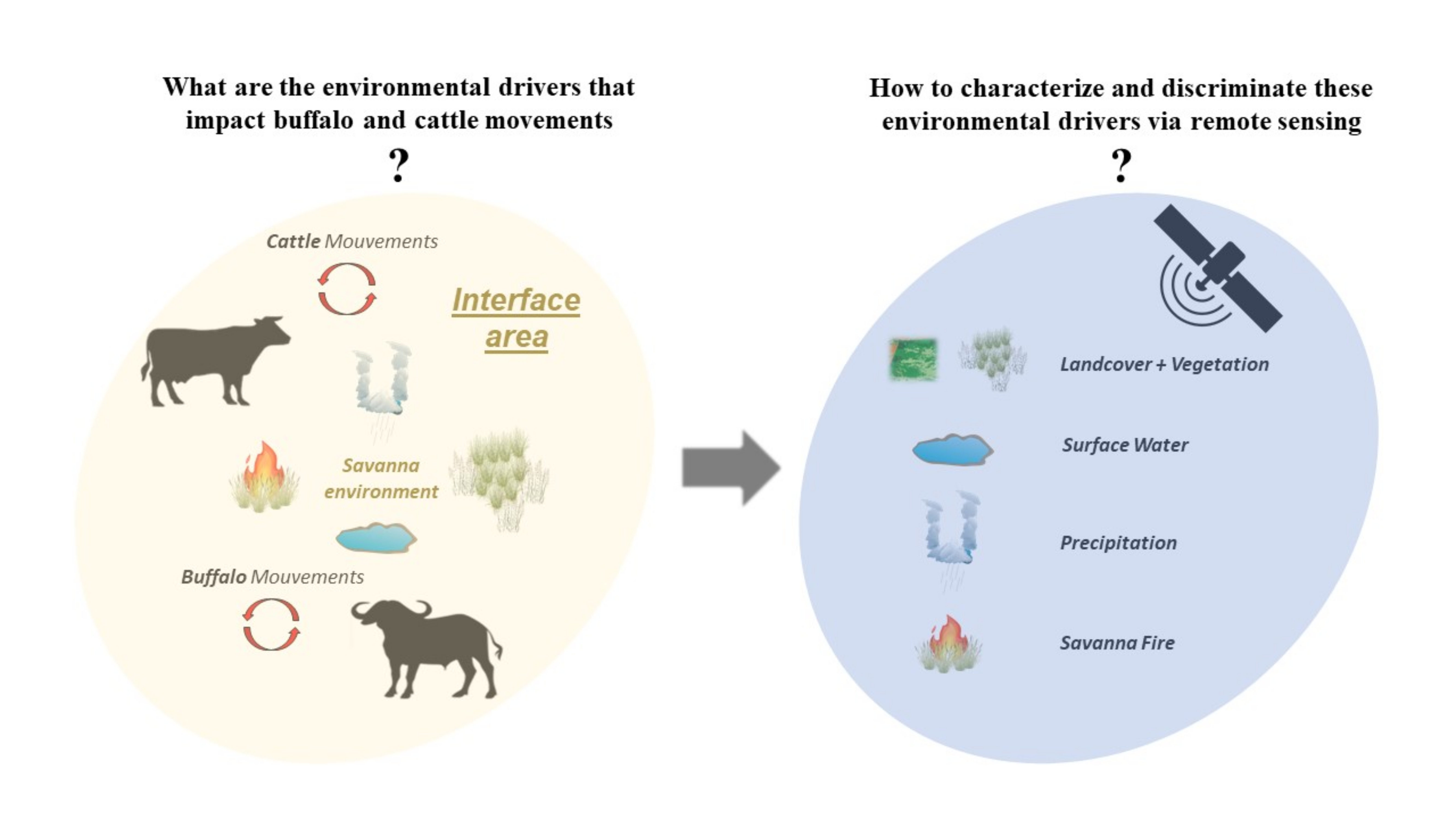
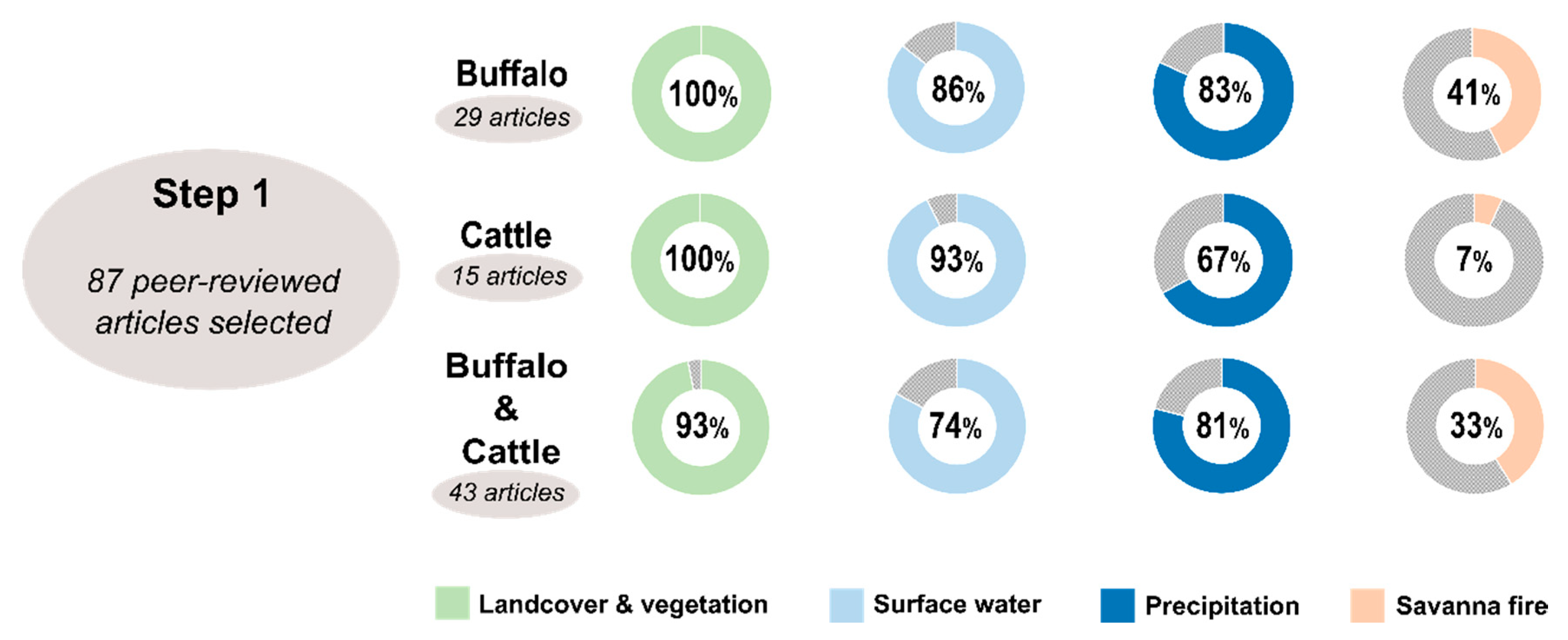
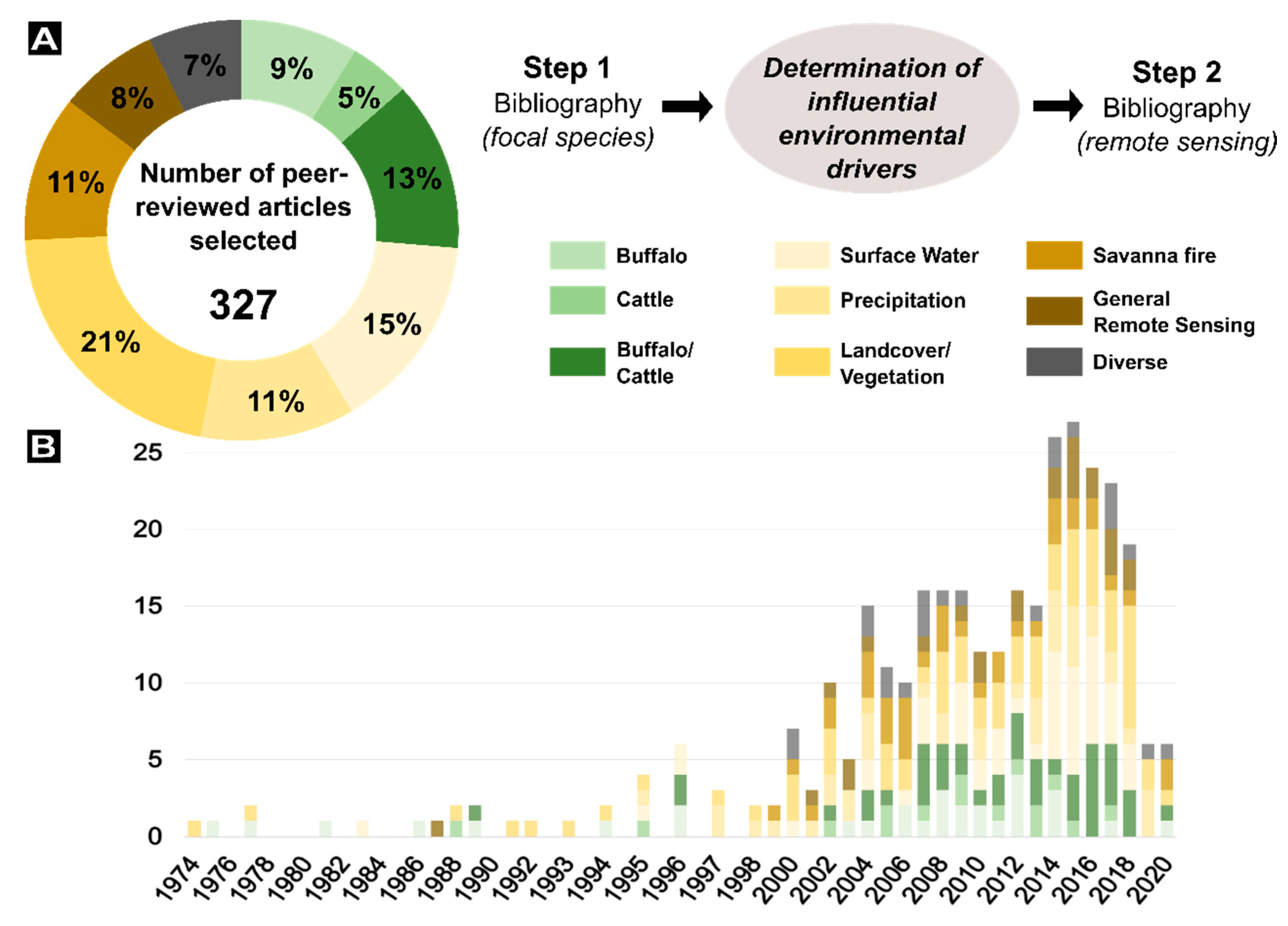
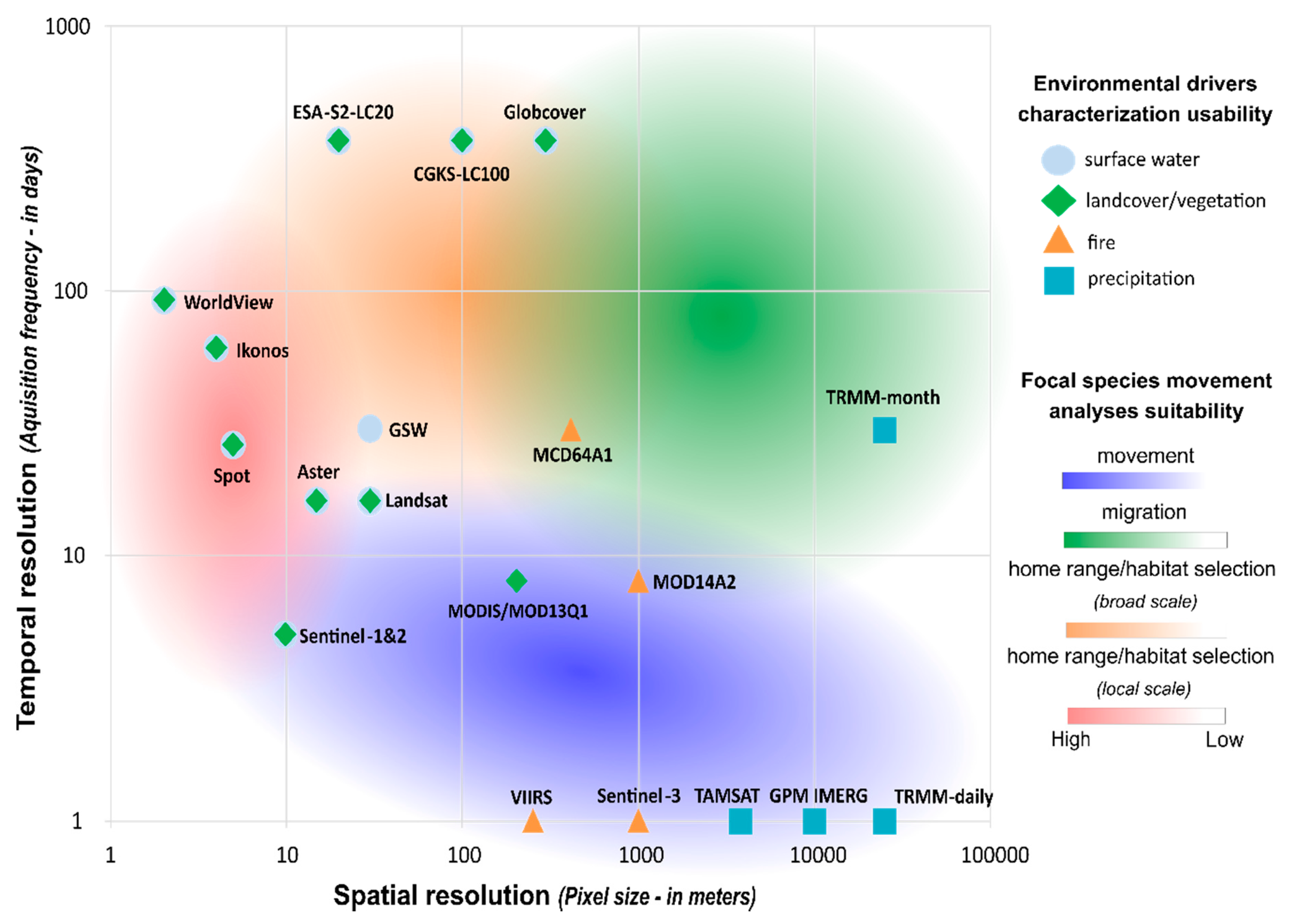
| Optical Remote Sensing Satellites | |||||||
| Sensor Resolution | Satellite | Spatial Resolution | Revisit Time Period | Nb of Spectral Bands | Access | Data Availability | Used in Buffalo/Cattle Ecological Studies |
| Low Resolution | NOAA | 1.1 Km | 2 times a day | 5 | Open-source | 1978–present | [86,87] |
| MODIS | Bands 1–2 250 m/bands 3–7 500 m/bands 8–36 1 km | 2 times a day | 36 | Open-source | 1999–present | [29,54,67,79,87,88,89] | |
| Suomi NPP | Bands I1-5 375 m/bands M1-16 750 m | 2 times a day | 22 | Open-source | 2012–present | - | |
| Envisat MERIS | 300 m | 3 days | 15 | Open-source | 2002–2012 | - | |
| Sentinel-3 | 300 m | 2 days | 21 | Open-source | 2016–present | - | |
| Medium Resolution | Landsat | Pan* 15 m/MS* 30 m/TIR* 60 to 100 m | 16 days | 4–11 | Open-source | 1972–present | [11,37,88,90] |
| Sentinel-2 | VNIR* 10 m/SWIR* 20 m/ACB* 60 m | 5 days | 13 | Open-source | 2015–present | [91] | |
| Aster | VNIR 15 m/SWIR 30 m/TIR 90 m | 16 days | 14 | Open-source | 1999–present | - | |
| High Resolution | Spot | Pan 1.5 to 2.5 m/MS 6 to 10 m | 26 days | 4–5 | Licensed | 1986–present | [26] |
| Ikonos | Pan 1 m/MS 4 m | 1.5–3 days | 5 | Licensed | 1995–2015 | [54,92] | |
| Rapideye | MS 5 m | 1–5.5 days | 5 | Licensed | 2008–present | [26] | |
| ZY-3 | Pan 2.1 m/MS 5.8 m | 5 days | 4 | Licensed | 2012–present | - | |
| GF-1/GF-2 | MS 5 m | 4–5 days | 5 | Licensed | 2013–present | - | |
| Planetscope-DOVEs | MS 3 m | Daily | 4 | Licensed | 2017–present | - | |
| Very-high Resolution | Quickbird | Pan 0.61 m/MS 2.24 m | 2.7 days | 5 | Licensed | 2001–2015 | - |
| WorldView | Pan 0.31 m/MS 1.24 m | 1–4 days | 4–17 | Licensed | 2007–present | [79] | |
| Geoeye | Pan 0.41/MS 1.64 m | 3 days | 5 | Licensed | 2008–present | - | |
| Pleaides | Pan 0.7 m/MS 2.8 m | Sub-daily | 5 | Licensed | 2011–present | - | |
| Skysat | Pan 0.9 m/MS 2 m | Sub-daily | 5 | Licensed | 2013–present | - | |
| Radar Remote Sensing Satellites | |||||||
| Satellite | Frequency | Spatial Resolution | Revisit Time Period | Polari-zation | Access | Data Availability | Used in Buffalo/Cattle Ecological Studies |
| ERS-1/ERS-2 | C-band (5.3 GHz) | 30 m | 35 days | VV | Open-source | 1991–2001 | - |
| Radarsat 1 Radarsat 2 | C-band (5.3 GHz) C-band (5.405 GHz) | 50 m 25 m | 24 days 24 days | HH VV-VH | Open-source Licensed | 1995–present 2007–present | - - |
| Envisat ASAR | C-band (5.3 GHz) | 12.5 m | 35 days | VV | Open-source | 2002–2012 | - |
| TerraSAR-X/TanDEM-X | X-band (9.6 GHz) | 5 m | 11 days | HH-VV | Licensed | 2007–present | - |
| Sentinel-1 | C-band (5.405 GHz) | FR* 3.5 m/HR* 10 m and 25 m/MR* 25 m and 40 m | 6 days | VV-VH | Open-source | 2014–present | - |
| Alos PALSAR 1-2 Alos PALSAR 2 | L-band (1.27 GHz) | SP* 9 × 10 m/DP* 19 × 10 m | 46–14 days | VV VH HH HV | Licensed | 2006–present | - |
| Product Name | Spatial Resolution | Data Availability | Sensor Used | Reference |
|---|---|---|---|---|
| Climate Change Initiative (CCI) LandCover V2 | 300 m | 1992 to 2015–2016–2017–2018 | MERIS Full and Reduced resolution/Spot VGT | [114] |
| MCD12Q1 0.5 km MODIS-based Global LandCover | 500 m | 2001–today | MODIS | [115] |
| Globeland30 | 30 m | 2000/2010 | Landsat TM, ETM7, HJ-1A/b | [116] |
| GLC 2000 | 1 km | 2000 | SPOT 4 VEGETATION | [117] |
| GlobCover 2005 V2.2 2009 | 300 m | 2005/2009 | MERIS FR | [118] |
| GLCNMO V.1-V.2-V3 | 1 km/500 m | 2003/2008/2013 | MODIS | [119] |
| GLC Share | 1 km | 2014 | MERIS-MODIS | [120] |
| GLC250 m CN (2001/2010) | 250 m | 2001/2010 | MODIS | [121] |
| FROM-GLC (GLC, GLC-seg, GLC-agg, GC, GLC-hierarchy) | 30 m | 2010 | Landsat TM, ETM+ | [122] |
| Global 30m Landsat Tree Canopy (TCC) V.4 | 30 m | 2000, 2005, 2010, and 2015 | MODIS, Landsat TM, ETM+ | [123] |
| Global Forest Change (GFC) - GLAD (Global Land Analysis & Discovery) lab at the University of Maryland (UMD) | 30 m | 2000 to 2019 | Landsat TM, ETM+, OLI | [80] |
| Copernicus Global 100 m Landcover (CGLS-LC100) | 100 m | 2015 | PROBA-V EO and GSD | [124] |
| ESA-S2-LC20, 20 m (over Africa) | 20 m | 2016 | Sentinel-2A | [125] |
| Spectral Index | Calculation * | Reference | Used in Buffalo/Cattle Ecological Studies |
|---|---|---|---|
| Normalized Difference Vegetation Index (NDVI) | [148,149] | [26,68,79,86,88,145,146,147] | |
| Enhanced Vegetation Index (EVI) | [150] | [29,54,89,146] | |
| Global Environmental Monitoring Index (GEMI) | [142] | - | |
| Soil Adjusted Vegetation Index (SAVI) | [143] | - | |
| Modified Soil Adjusted Vegetation Index (MSAVI) | [151] | - | |
| Modified Secondary Soil-Adjusted Vegetation Index (MSAVI2) | [152] | - | |
| Difference Vegetation Index (DVI) | [153] | - | |
| Optimized Soil-Adjusted Vegetation Index (OSAVI) | [154] | - | |
| Soil Brightness Index (SBI) | [155] | - | |
| Two-band Enhanced Vegetation Index (EVI2) | [156] | - | |
| Modified Chlorophyll Absorption Ratio Index (MCARI) | [157] | - |
| Spectral Index | Calculation* | Reference | |
|---|---|---|---|
| Normalized Difference Infrared Index | NDII | [185] | |
| Normalized Difference Vegetation Index | NDVI | [148,149] | |
| Enhanced Vegetation Index | EVI | [150] | |
| Normalized Difference Water Index | NDWI | [186] | |
| Normalized Difference Water Index (Gao) | NDWI (Gao) | [187] | |
| Modified Normalized Difference Water Index | MNDWI | [188,189] | |
| Normalized Difference Turbidity Index | NDTI | [188] | |
| Normalized Difference Phytoplankton Index | NDPI | [188] | |
| Automated Water Extraction Index | AWEInsh AWEIsh | AWEInsh = AWEIsh = | [190] |
| Water Index | WI | [191] | |
| Product Name | Developer | Spatial Resolution | Frequency | Data Availability | Reference |
|---|---|---|---|---|---|
| Global surface water (GSW) | EC JRC (European Commission Joint Research Center)/Google | 30 m | Monthly Yearly | 1984–2015 1984–2019 | [217] |
| CCI global map of open water bodies (WBP V4.0) | ESA (European Space Agency) - climate change initiative(CCI) | 300 m to 1 km | 7 days–1 year | 2000–2015 | [218] |
| Global lakes and wetlands database (GLWD) | University of Kassel/World Wildlife Fund (WWF) | 1 km | 1 year | 2004 | [219] |
| SRTM water body data product specific guidance (SWBD) | National Aeronautics and Space Administration (NASA) | 90 m | 1 year | 2000 | [220] |
| SAR-Based water body indicator (SAR-WBI) | ESA | 150 m to 1 km | 6 to 12 days | 2005–2012 | [221] |
| MOD44W | NASA | 250 m | yearly | 2000–2015 | [222] |
| Copernicus WB | Copernicus program-ESA | 300 m to 1 km | 10 days | 2014–present | [223] |
| Global 3-s/1-s water body map (G3WBM/G1WBM) | Department of Integrated Climate Change Projection Research, 4 Japan Agency for Marine-Earth Science and Technology | 30 m to 90 m | 1 year | 2018 | [224] |
| Product Name | Spatial Resolution | Orbital Frequency | Data Availability | Reference | Use in Ungulates Ecological Studies |
|---|---|---|---|---|---|
| MOD14A2/MYD14A2 | 1 km | Every 8 days | 2000–present | [252] | [29] |
| MCD45A1 | 500 m | Monthly | 2000–present | [253] | - |
| MCD64A1 | 500 m | Monthly | 2000–present | [248] | - |
| VIIRS 750 m active fire (VNP14) | 750 m | twice/day (IR and day/night VIS/NIR channel) once/day (VIS) | 2011–present | [254] | - |
| VIIRS 375 m Active Fire (VNP14IMG) | 375 m | twice/day (IR and day/night VIS/NIR channel) once/day (VIS) | 2016–present | [238] | - |
| Sentinel-3 SLSTR (level-2 FRP product) | 1 km | Daily | 2018–present | [255] | - |
| AVHRR Fire Detects from the Fire Identification, Mapping and Monitoring Algorithm (FIMMA) | 1 km | Daily | 1978–present | [256] | - |
| ESA FIRE_CCI | 300 m | Monthly | 2016–present | [257] | - |
| FireCCI51 | 250 m | Monthly | 2001–2019 | [258] | - |
| Spectral Index | Calculation * | Reference |
|---|---|---|
| Normalized Burned Ratio (NBR) | [258] | |
| Burned Area Index (BAI) | [259] | |
| Mid Infrared Burned Index (MIRBI) | [260] | |
| Char Soil Index (CSI) | [261] | |
| Normalized Burn Ratio Thermal (NBRT) | [262] | |
| Normalized difference Vegetation Index Thermal (NDVIT) | [262,263] |
| Product Name | Temporal Resolution | Spatial Resolution | Data Availability | Coverage | In-Situ Calibration | Reference | Use in Ungulates Ecological Studies |
|---|---|---|---|---|---|---|---|
| TRMM (TMPA 3B42 V7) | 3 h | 0.25° | 1998–Mid 2019 | 50°S–50°N | yes | [288] | [29,146] |
| TRMM (TMPA 3B43 V7) | Monthly | 0.25° | 1998–Mid 2019 | 50°S–50°N | yes | [288] | [29,146] |
| PERSIANN-CDR | Hourly/Daily/ Monthly/yearly | 0.25° | 1983–present | 60°S–60°N | no | [289] | - |
| GPCP (1dd) | Daily | 1° | 1996–present | 90°S–90°N | no | [290] | - |
| GPCP V2.3 | Monthly | 2.5° | 1979–present | 90°S–90°N | no | [291] | - |
| CPC Global | Daily | 0.5° | 1979–present | 90°S–90°N | yes | [292] | - |
| CMAP | Monthly | 2.5° | 1979–present | 90°S–90°N | yes | [293] | - |
| Cmorph | 30 min | 0.25° | 2002–2017 | 60°S–60°N | no | [294] | - |
| GPM (IMERG V06) | 30 min/3 h/Daily | 0.1° | 2000–present | 60°S–60°N | no | [295] | - |
| MSWEP V2 | 3 h/Daily | 0.1°/0.5° | 1979–2017 | 90°S–90°N | yes | [296] | - |
| SM2RAIN-ASCAT | Daily | 0.5° | 2007–2018 | 60°S–60°N | no | [297] | - |
| TAMSAT V3.1 | Daily | 0.0375° | 1983–present | 38°025N–35°9625S 19°0125W–51°975E | yes | [62,63] | - |
| CHIRPS v2p0 | Daily | 0.05° | 1981–present | 50°S–50°N | yes | [298] | - |
| ARC V.2 | Daily | 0.1° | 1983–present | 40°S–40°N | yes | [299] | - |
| RFE 2.0 | Daily | 0.1° | 2001–present | 40°S–40°N 20°W–55°E | yes | [300] | - |
| EPSAT-SG | 15 min | 0.0375° | 2004–present | African continent | yes | [301] | - |
| MPE | 15 min | 0.0375° | 2007–present | African & European continents | no | [302] | - |
© 2020 by the authors. Licensee MDPI, Basel, Switzerland. This article is an open access article distributed under the terms and conditions of the Creative Commons Attribution (CC BY) license (http://creativecommons.org/licenses/by/4.0/).
Share and Cite
Rumiano, F.; Wielgus, E.; Miguel, E.; Chamaillé-Jammes, S.; Valls-Fox, H.; Cornélis, D.; Garine-Wichatitsky, M.D.; Fritz, H.; Caron, A.; Tran, A. Remote Sensing of Environmental Drivers Influencing the Movement Ecology of Sympatric Wild and Domestic Ungulates in Semi-Arid Savannas, a Review. Remote Sens. 2020, 12, 3218. https://doi.org/10.3390/rs12193218
Rumiano F, Wielgus E, Miguel E, Chamaillé-Jammes S, Valls-Fox H, Cornélis D, Garine-Wichatitsky MD, Fritz H, Caron A, Tran A. Remote Sensing of Environmental Drivers Influencing the Movement Ecology of Sympatric Wild and Domestic Ungulates in Semi-Arid Savannas, a Review. Remote Sensing. 2020; 12(19):3218. https://doi.org/10.3390/rs12193218
Chicago/Turabian StyleRumiano, Florent, Elodie Wielgus, Eve Miguel, Simon Chamaillé-Jammes, Hugo Valls-Fox, Daniel Cornélis, Michel De Garine-Wichatitsky, Hervé Fritz, Alexandre Caron, and Annelise Tran. 2020. "Remote Sensing of Environmental Drivers Influencing the Movement Ecology of Sympatric Wild and Domestic Ungulates in Semi-Arid Savannas, a Review" Remote Sensing 12, no. 19: 3218. https://doi.org/10.3390/rs12193218
APA StyleRumiano, F., Wielgus, E., Miguel, E., Chamaillé-Jammes, S., Valls-Fox, H., Cornélis, D., Garine-Wichatitsky, M. D., Fritz, H., Caron, A., & Tran, A. (2020). Remote Sensing of Environmental Drivers Influencing the Movement Ecology of Sympatric Wild and Domestic Ungulates in Semi-Arid Savannas, a Review. Remote Sensing, 12(19), 3218. https://doi.org/10.3390/rs12193218