Article

Stereo Dense Image Matching by Adaptive Fusion of Multiple-Window Matching Results

1
School of Remote Sensing and Information Engineering, Wuhan University, Wuhan 430079, China
2
Department of Civil, Environmental and Geodetic Engineering, The Ohio State University, Columbus, OH 43221, USA
3
Department of Electrical and Computer Engineering, The Ohio State University, Columbus, OH 43221, USA
4
Translational Data Analytics, The Ohio State University, Columbus, OH 43221, USA
*
Author to whom correspondence should be addressed.
Remote Sens. 2020, 12(19), 3138; https://doi.org/10.3390/rs12193138
Submission received: 24 August 2020 / Revised: 16 September 2020 / Accepted: 22 September 2020 / Published: 24 September 2020

Abstract

:
Traditional stereo dense image matching (DIM) methods normally predefine a fixed window to compute matching cost, while their performances are limited by the matching window sizes. A large matching window usually achieves robust matching results in weak-textured regions, while it may cause over-smoothness problems in disparity jumps and fine structures. A small window can recover sharp boundaries and fine structures, while it contains high matching uncertainties in weak-textured regions. To address the issue above, we respectively compute matching results with different matching window sizes and then proposes an adaptive fusion method of these matching results so that a better matching result can be generated. The core algorithm designs a Convolutional Neural Network (CNN) to predict the probabilities of large and small windows for each pixel and then refines these probabilities by imposing a global energy function. A compromised solution of the global energy function is utilized by breaking the optimization into sub-optimizations of each pixel in one-dimensional (1D) paths. Finally, the matching results of large and small windows are fused by taking the refined probabilities as weights for more accurate matching. We test our method on aerial image datasets, satellite image datasets, and Middlebury benchmark with different matching cost metrics. Experiments show that our proposed adaptive fusion of multiple-window matching results method has a good transferability across different datasets and outperforms the small windows, the median windows, the large windows, and some state-of-the-art matching window selection methods.

Graphical Abstract

1. Introduction

The goal of stereo dense image matching (DIM) is to find pixel-wise correspondences between stereo image pairs, which has been attracting increased attention in photogrammetry and computer vision communities for decades [1,2]. The image pairs are generally rectified in the epipolar image space such that correspondences are in the same row between the pairs with only differences in the column coordinates, termed disparity or parallax. Therefore, DIM often refers to computing disparities for each pixel in one of the epipolar image pairs (typically the left image), thus forming a disparity image. DIM is a popular technique to obtain three dimensional (3D) information at low cost, and it has fueled many geoscience applications, including autonomous driving, robotic navigation, Digital Surface Model (DSM) generation, 3D reconstruction, and automated mapping [3,4,5,6,7,8,9].
Traditional DIM methods search correspondences by comparing the similarities of their appearances (e.g., intensities, textures). Most DIM methods [10] predefine a fixed window to describe the appearance features of correspondences, and compare the appearance similarities by measuring distances of these features, also termed as matching cost. Various window-based matching metrics have been proposed in the last decades, and the difference among them mainly focused on the various appearance feature descriptors, e.g., image intensities, image gradients, and intensity rankings. Image intensity-based matching cost metrics [1,11,12] assume brightness constancy for correspondences and compute matching cost by comparing intensities in matching windows of correspondences. Such methods are always efficient and straightforward, but sensitive to noises and image radiometric distortions. Image gradient-based matching cost metrics compute gradients for each pixel, and either use these gradients themselves or use the distributions of these gradients as feature descriptors [13,14,15,16]. Such methods can compensate for linear radiometric distortions between correspondences and achieve robust matching results in textured regions. Intensity ranking based matching cost [17,18,19,20] ranks intensities within a matching window by comparing these intensities with the central pixel and considers the ranking results as the feature descriptors. Among such methods, Census [17,21] may be the most commonly used matching cost and has been proven to be one of the most robust when compared with other traditional methods [1].
Most DIM methods use a fixed window to compute matching cost, while their performances are limited by matching window sizes. A large window (e.g., 15 × 15 pixels) provides more information for feature descriptors such that its matching results contain few uncertainties, especially in weak-textured regions (white rectangles in Figure 1c). However, it may cause over-smoothness issues in fine structures (black rectangles in Figure 1c). A small window (e.g., 5 × 5 pixels) can compute more accurate matching results in disparity jumps as well as fine structures (black rectangles in Figure 1b), while it also contains high matching uncertainties in weak-textured/untextured regions (white rectangles in Figure 1b). Therefore, the matching results with large windows and small windows can complement each other, thus raising a problem: is it possible to fuse the matching results of large windows and small windows for a higher-accuracy result?
This paper particularly addresses the above issues by training a Convolutional Neural Network (CNN) with the underlying assumption that matching window size is dependent on disparity changes and textures within the window. We develop a method that estimates appropriate weights of different matching windows in the fusion of the matching results, termed as adaptive matching results fusion based on a Convolutional Neural Network (AMF-CNN). The core algorithm predicts the probabilities of large and small windows from the network. It then refines these probabilities by formulating the matching window selection problem as the optimization of a global energy function, thus being able to reduce some misestimation/noises in the probability estimation results of the network. A compromised solution of the global energy function is utilized by breaking the optimization into a collection of sub-optimizations of pixels in one-dimensional (1D) paths. Considering the uncertainties in window size estimation, we fused large and small windows by formulating the refined probabilities as weights for more accurate matching results. The main contributions of our method include:
(1)
Our proposed method utilizes intensity and disparity information to predict the appropriate weights of large and small windows in the fusion.
(2)
Our proposed method leverages the advantages of small and large matching windows and achieves the most accurate matching results when compared with small, large, and median matching window sizes as well as some state-of-the-art window selection methods.
(3)
Our proposed method provides good transferability across different datasets. The network is trained by a street view dataset, while the testing datasets are indoor images, aerial images, and satellite images.
The remainder of the paper is organized as follows: Section 2 introduces an overview of related works. Section 3 describes the methodology of the proposed method in detail. In Section 4, we validate our proposed method by assessing it with fixed window size and other state-of-the-art window selection methods on all platform images, including indoor/aerial/satellite datasets. We discuss the performance and transferability of our method. Section 5 concludes our work by highlighting our contribution of the proposed method in this paper.

2. Related Work

In recent years, there have been several attempts to improve the matching results by adaptively selecting matching windows or fusing the matching results of multiple windows. The basic idea is that the matching window sizes or the fusion weights of different windows are dependent on the textures and disparities. In weak textures or small disparity changes (<1 pixel), a large window is preferred to contain sufficient image information, while in edges or fine structures, a small window is preferred for fitting the local disparity changes. Either image or disparity can be used to select appropriate matching windows; therefore, the matching results fusion methods of multiple windows can be categorized into (1) disparity-based method, (2) image-based method, and (3) the comprehensive method.
Disparity-based methods [20,24,25] typically select large windows in disparity-consistency regions and small windows in disparity discontinuities. Erway and Ransford proposed an iterative strategy that firstly selected matching windows based on the initial disparity image, computed a more accurate disparity image using the adaptive window, then selected new matching windows based on the more accurate disparity image and iterated on [24]. Lin et al. [25] computed disparities with different window sizes and adaptively selected windows that meet the disparity consistency constraints. However, such methods are limited by matching accuracies of the initial disparity images. Mismatches in disparity images may lead to inappropriate window sizes.
Image-based methods utilize some image clues (including edges and textures) for window selection. In such methods, image edges are firstly detected, then the corresponding edge pixels are assigned small matching windows to guarantee high matching accuracies in edges, and the remaining non-edge pixels are assigned larger windows for robust matching [26,27]. Image texture is an alternative way to decide windows. Several works [25,28,29] describe image textures by gradients, texture entropy, signal to noise ratio (SNR), and assign smaller windows to pixels in textured regions and larger windows to pixels in weak-textured regions. Such methods are independent of initial disparity images, while images sometimes may give wrong clues. For example, the detected edges may not be disparity discontinuities, or disparity discontinuities occur in weak textures, in which cases the wrong clues may lead to inappropriate window sizes.
Considering the limitations of both disparity-based methods and image-based methods, researchers proposed comprehensive methods leveraging both disparity and image information for window selection. Kanade and Okutomi made a pioneering work by statistically formulating local variations of image intensities and disparities as the uncertainty in disparity estimations within different windows and selecting the window with the least uncertainties [30]. Adhyapak et al. used matching cost, a function of image intensities and disparities, to evaluate the uncertainties of each matching window [31]. They used several metrics (e.g., the number of local minimums of matching cost and the local variation around the minimum matching cost) to evaluate the matching uncertainties of windows with different sizes, and then selected window with the least uncertainties. The window selection of such methods depends on the uncertainties evaluation results. However, the metrics in [30,31] only extracted low-level features of textures and disparities, which are too simple to describe the complicated relationship between the texture/disparity and the window size. In early 2020, we [32] proposed a matching window size selection network, which extracts in-depth features of images and disparities, thus computing more accurate matching window selection results. Compared with the previous work, the main differences and improvements include: (1) in the previous work, only one window is selected in the matching of each pixel. The single-window matching results are sometimes unreliable, though the matching windows are already optimal. Instead, our new work fuses the matching results of multiple windows, thus generating more robust matching results. (2) The window size prediction results from CNN in the previous work may still have some noises. We, therefore, optimized the window size prediction results in the new work with the underlying assumption that the fusion weights of adjacent pixels with similar intensities should be similar.

3. Methodology

3.1. Overall Scheme

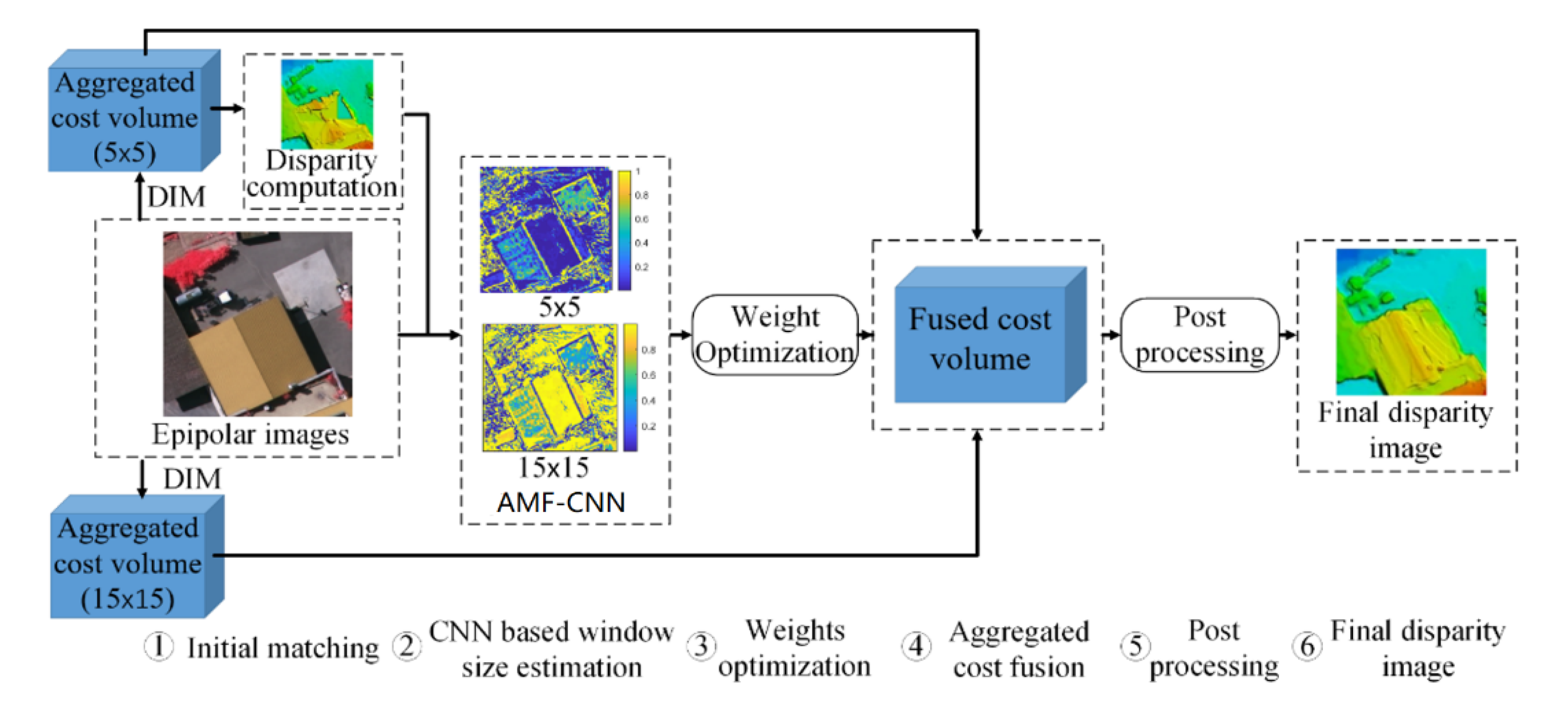
For accurate matching, we consider both texture and disparity information and develop a method to adaptively fuse matching results of different matching windows by training a convolutional neural network. However, it is expected that some inappropriate fusion weights estimation results may exist due to the mismatches in initial disparities or some radiometric distortions in textures. To get more robust weights estimation results, we propose a workflow that formulates the window weights estimation problem as the optimization of a global energy function with a compromised solution that breaks the optimization into a collection of sub-optimization in 1D paths. We can also acquire more robust weights of large and small windows after the optimization and then use these weights to fuse the matching results of large windows and small windows for more accurate disparities, as shown in Figure 2.
Our proposed method adopted the famous semi-global matching (SGM) [23,33] to compute pixel-wise disparities, which formulates stereo dense image matching as the optimization of a global energy function in two-dimensional (2D) image space. However, the optimal solution of the energy function is a typical NP-hard (Non-deterministic Polynomial-time hard) problem, which is difficult to obtain in polynomial time. Therefore, SGM breaks the global optimization into sub-optimizations in 1D paths. The solutions of these sub-optimizations are computed by aggregating matching costs along the 1D paths with dynamic programming functions. After the 1D cost aggregations, each pixel has aggregated matching cost at all disparities, thus forming a cost volume. These cost volumes of the 1D path aggregations are then accumulated to generate the final aggregated cost volume in 2D image space, and the approximate global solution of the global energy function is finally computed by deriving disparities with respect to the minimum aggregated cost in the aggregated cost volume. Based on SGM, our proposed method consists of five main components:
Initial matching: we presume the availability of epipolar stereo images and use semi-global matching (SGM) [23] with different matching window sizes (15 × 15 pixels and 5 × 5 pixels) to compute aggregated matching cost volumes of left or right images. The initial disparity images can be derived from any one of the aggregated cost volumes (e.g., 5 × 5 pixels cost volumes in this paper).
Window weights estimation from the convolutional network: we respectively estimate probabilities of large or small windows by training a convolutional neural network. Since we will use the probabilities as weights in the fusion of the finial matching results, we also term the window probabilities as windows weights in the remaining paper.
Weights optimization: we formulate the window weight estimation problem as a global energy function and develop a comprised solution to compute more robust window weights.
Aggregated cost fusion: considering uncertainties in matching, aggregated cost volumes of large and small windows are weighted fused for more accurate matching.
Disparity computation and post-processing: after computing fused matching cost volumes for left and right images, disparities of left and right images can be derived by winner-takes-all (WTA) strategy, then mismatches are detected and eliminated by left-right consistency check (LRC), leaving holes in disparity images, which are finally interpolated by discontinuity preserving interpolation [23].

3.2. Proposed Method

Given a pair of epipolar images I = { I L , I R }   ( I L : left image,   I R : right image), we formulate the window size estimation as a labeling problem and assign binary labels for each pixel: small windows (e.g., 5 × 5 pixels) and large windows (e.g., 15 × 15 pixels). To solve such a problem, a global energy function E , which considers the window size consistency between adjacent pixels, is then built, as shown in Equation (1). The optimal solution is typically acquired by minimizing the global energy function:
min E ( L ) = E d a t a ( L ) + E s m o o t h ( L ) ,
where L is a set of estimated window sizes for each pixel; E d a t a   measures the large and small window weights for each pixel termed as data term; E s m o o t h is a regularization term that imposes the window size consistency constraints over the entire label set L .
The data term E d a t a ( L ) is a function of matching window sizes based on variations of image intensities and disparities. In general, it calculates, for every pixel, the cost of selecting small or large windows, which is an actually negative correlation to the window weights, and then sums these window selection costs across the entire image as the data term to this energy function, as shown in Equation (2). In our method, we design a CNN-based network for estimating the windows weights, which will be described in Section 3.2.1.
E d a t a ( L ) = p I b ( 1 C N N ( p , W l p ( d ) ,   W l p ( I ) ) ) = p I b c o s t ( p , l p ) ,
where I b is the set of all pixels in a base image (e.g., the left); p is a pixel in the base image; l p is the estimated window size of pixel p; W l p is the window centered at p with size l p ; W l p ( d ) is a set of initial disparities within the window W l p ; W l p ( I ) is a set of image intensities within the window W l p ; c o s t ( p , l p ) means the cost of selecting W l p as the matching window.
Since we only consider disparities and intensities in local windows, E d a t a may contain some uncertainties. Therefore, a regularization term E s m o o t h is built to impose the smoothness over the entire set L with the underlying assumption that adjacent pixels with similar color/intensities should share the same window sizes, defined as the first-order derivatives of L :
E s m o o t h ( L ) = p , q N P · w ( p , q ) · | l p l q | ,
where p , q are neighboring pixels in the image; N is the set of adjacent pixels; w ( p , q ) is the weight controlling the smoothness constraints based on the intensity differences of neighboring pixels. The weight is inversely proportional to their intensity differences. P is a penalty factor controlling the extent of smoothness between adjacent pixels. In this paper, we utilize a comprised solution that breaks the optimization of the energy function into the collections of sub-optimizations in 1D paths. We can also acquire more robust window weights from the solution. These more robust window weights can be used in the fusion of aggregated matching cost volumes. The comprised solution will be introduced in Section 3.2.2.

3.2.1. Adaptive Matching Fusion based on Convolutional Neural Network (AMF-CNN)

Training Data Generation: Our training data are generated from the KITTI stereo 2012 dataset [34], where 185 image pairs are selected except for the other nine pairs, which are too dark or bright. Three different matching cost metrics (Census [17], Zero mean Normalized Cross-Correlation (ZNCC) [35] and MC-CNN-fst [22]) with two different window sizes (5 × 5 and 15 × 15 pixels) are used to compute the disparity images of the 185 pairs with SGM optimization. Since the original version of MC-CNN-fst was trained from a 9 × 9 pixels window, we implement MC-CNN-fst with a 5 × 5 pixels window and 15 × 15 pixels window by resizing the original images. To ensure the dependence of the training data labels on window sizes except for some particular matching cost metrics, we select pixels with consistent matching accuracies among all matching cost metrics of large or small windows as training samples. In general, positive samples are the pixels whose estimated disparities of the three matching cost metrics in large windows are closer to truth disparities than those in small windows. Conversely, negative samples are defined from the pixels whose estimated disparities of the three matching cost metrics in small windows are closer.
Considering the class balance of the training samples, we take the same number of positive and negative samples. Under this strategy, about 500,000 pixels are extracted from the KITTI 2012 dataset for training. Considering the consistent matching accuracies among all matching cost metrics, only a small percentage of pixels can fit our sample selection strategy. To make sure the number of training data is large enough for training, we use the disparity results after SGM optimization (with LRC) with two matching window sizes to generate the training data. The 185 image pairs of KITTI 2012 are standardized for data augmentation. Since matching window sizes are dependent on both image textures and disparity variations, we extract textures and disparities information of these training sample pixels by intercepting regular patches around these pixels in intensity images and disparity images. To accurately extract texture features in different windows, we intercept the 5 × 5 and the 15 × 15 pixel patches from the left image centered at these training sample pixels. The extraction of disparity patches is similar to image patches. However, due to the sparsity of the original true disparity images in KITTI 2012, it is possible that only a few valid disparities exist in small windows so that disparity variations cannot be accurately evaluated. Therefore, the sparse true disparity images are firstly interpolated into dense disparity images by triangulation. Then, the 5 × 5 and the 15 × 15 pixel patches from the interpolated true disparity images are extracted for measuring disparity variation of training sample pixels in different windows. Considering that the disparity interpolation is not able to recover details in disparities, we only use the disparity differences by comparing the maximum disparities and minimum disparities in a patch as the input feature, as shown in Figure 3. Considering disparity jumps, we need to define a truncated value α to cut off the disparity differences larger than α. Traditional DIM methods [23] define α as 1 pixel. However, in slanted regions, the disparity differences of matching windows, especially the larger windows, may often be larger than 1 pixel. Thus, we empirically define α as 5 pixels, because the disparity differences larger than 5 pixels are more likely to be disparity jumps. Finally, we normalize all the disparity differences in a range of [0, 1].
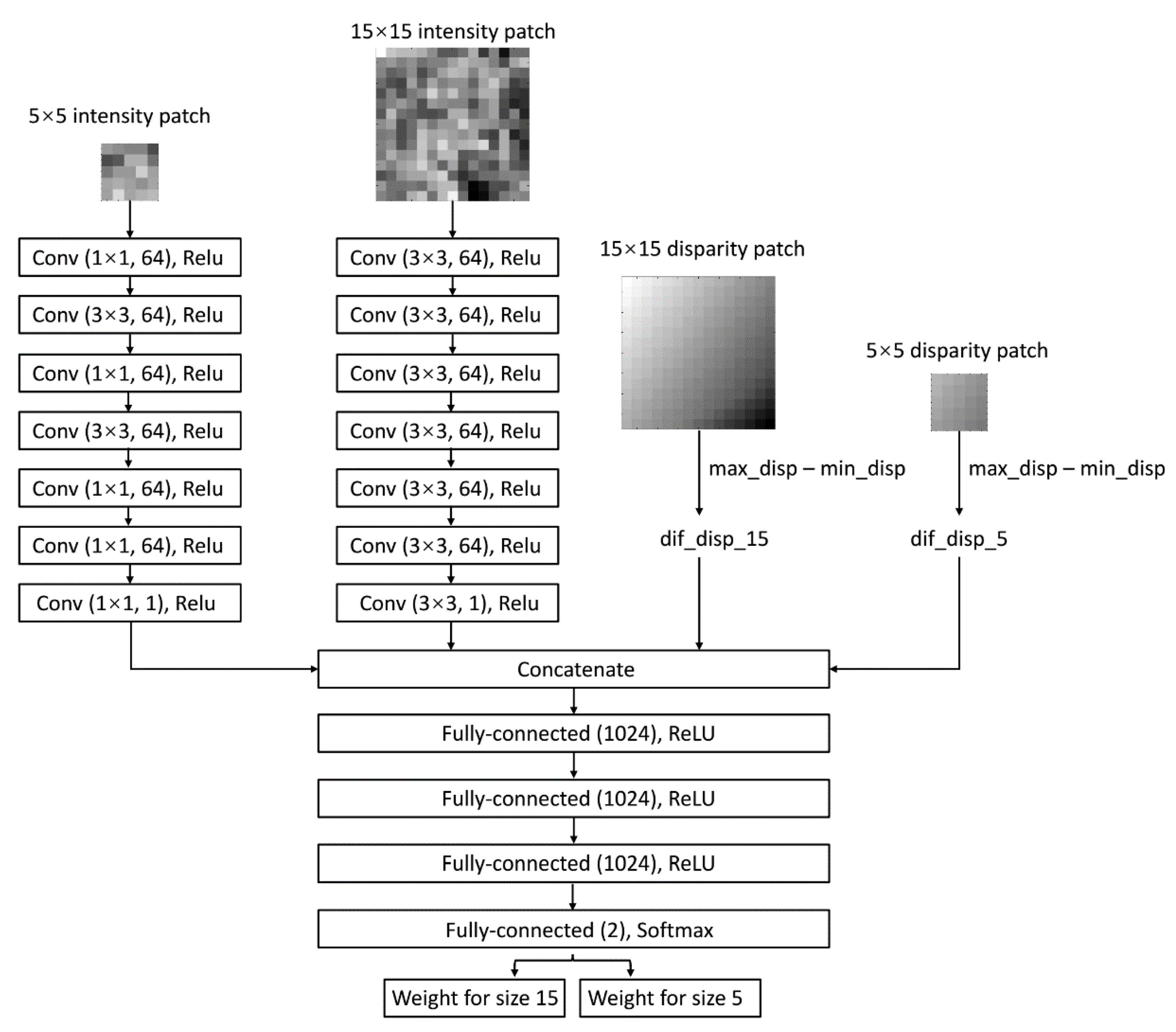
Details of Network Structure: The structure of our network is shown in Figure 3. For the branch of 15 × 15 image patch, seven convolutional layers with following rectified linear units (ReLU) are used to extract texture features. For the branch of the 5 × 5 image patch, we use some 1 × 1 convolutional layers to make sure the number of layers for the 5 × 5 image patch is as same as the 15 × 15 image patch. Since the disparity difference feature is one dimension, we also compress the patch texture feature as a one-dimension feature in the last convolutional layer. The resulting features extracted from a 5 × 5 image patch and a 15 × 15 image patch are concatenated with the disparity difference features in 15 × 15 and 5 × 5 disparity patches. Then, these features are forward-propagated through four fully connected layers, followed by ReLU. After being transformed with the softmax function, the last fully connected layer produces two probability numbers, which are interpreted as weights for the 15 × 15 window and 5 × 5 window, which are then used as data terms in the global energy function.
We use the cross-entropy loss and a momentum optimizer (momentum = 0.9) with an initial learning rate of 0.003 for training. The learning rate decay factor is set as 0.9 after 10 epochs, and the final model parameters are acquired after 50 epochs.

3.2.2. Solution for the Regularization Term

Since these window weights are estimated locally by image patches and disparity patches, some misestimates exist. Therefore, we need to impose the smoothness constraints over the entire window size set L and obtain the optimal solution of the global energy function in Equation (1). For the cost volumes fusion, we must acquire more robust window weights in addition to the optimal solution of the global energy function. Thus, we use a fast bilateral filtering strategy [36] instead of a typical graph cuts method [37] to compute robust weights of both window sizes. Fast bilateral filtering is usually used in the optimization of stereo dense image matching, which assumes that neighboring pixels with similar intensity should have the same disparities. Different from the traditional fast bilateral filtering methods, we introduced a stricter spatial constraint in the filtering and applied the filtering in the optimization of the matching window selection, where the window selection cost in Equation (2) of each pixel is refined by the surrounding pixels with similar intensities, thus being able to provide more robust window weights after the optimization. In general, fast bilateral filtering breaks the optimization of the global energy function into a collection of sub-optimizations in 1D paths and computes the sub-optimization in a propagation manner. However, in weak-textured regions, the inner pixels may give wrong clues to the edge pixels. Therefore, we add a spatial control factor in the propagation function to avoid the problem mentioned above:
L r ( p , l p ) = c o s t ( p , l p ) + T · w ( p , p r ) · L r ( p r , l p ) ,
where r is the direction of propagation path (e.g., the horizontal direction); L r is the propagated cost in direction r ; p is a pixel in the base image; p r is the previous pixel of p in direction r ; w ( p , p r ) is the intensity weight, which is inversely proportional to the intensity difference between p and p r . w ( p , p r ) is generally defined as Gaussian function. T is a controlling factor that is used to reduce the wrong cost propagation in edges of weak-textured regions.
In fast bilateral filtering, the cost of each pixel is propagated through non-local, orthogonal scanning lines. In general, the cost propagation firstly proceeds in both horizontal ( r = 0 ° ) and the corresponding inverse direction (termed as −   r ) in Equation (4), and then the propagated cost in these directions are aggregated to get the sub-optimization in horizontal directions, as shown in Equation (5):
S r ( p , l ( p ) ) = L r ( p , l p ) + L r ( p , l p ) c o s t ( p , l p ) ,
where L r and L r are propagated cost in r and -   r directions; S r is the aggregated cost, which is the sum of the propagated cost in both directions. Since both L r ( p , l p ) and L r ( p , l p ) contain the cost of p , c o s t ( p , l p ) is subtracted in Equation (5) for eliminating the redundancy.
Similar to the cost propagation in r and −   r directions, the aggregated cost S r is then regarded as the new cost for propagation in the perpendicular direction r and r . The propagated costs in r and r are finally summed to yield the aggregated cost S r ( p , l p ) in a similar manner of Equation (5). S r ( p , l p ) is the final aggregation result in the first r and then r directions.
To keep normalized cost, we need to compute the corresponding aggregated intensity weights S r by setting the cost of each pixel as one and aggregated these costs in first r and then r directions. Finally, the normalized cost is computed by dividing S r using S r , and the robust window weights of each pixel can be computed by:
w r ( p , l p ) = 1 S r ( p , l p ) / S r ( p , l p ) ,
where w r ( p , l p ) is the robust window weights of pixel p with size l p .
Then, we fused the aggregated cost volumes of large and small windows according to these robust window weights after the optimization:
S ( p , d ) = ( w r ( p , l L ) · S L ( p , d ) + w r ( p , l S ) · S S ( p , d ) ) / ( w r ( p , l L ) + w r ( p , l S ) ) ,
where l L is large window size; l S is small window size; w r ( p , l L ) is large window weight of pixel p ; w r ( p , l S ) is small window weights of pixel p ; S L ( p , d ) is aggregated matching cost volume of large window; S S ( p , d ) is aggregated matching cost volume of small window; S ( p , d ) is the weighted fused matching cost volume.
Disparity images can be derived from the fused matching cost volume by Winner-Takes-All (WTA), and then the Left-Right Consistency (LRC) strategy is used to eliminate the mismatches; finally, discontinuity preserving interpolation is utilized for the final dense disparity image [23].

4. Experimental Results

4.1. Experimental Setup

In this paper, our training data are from the street-view dataset in the KITTI benchmark. To evaluate the transferability of AMF-CNN, we evaluated our proposed method on three different datasets: an indoor dataset from Middlebury Stereo [38], an aerial remote sensing image dataset from the ISPRS benchmark [39], and a satellite image dataset on Jacksonville [40,41]. All the image pairs in these datasets have been rectified to epipolar images before applying our proposed method. In general, we tested our proposed method on the above three datasets with three different matching cost metrics, Census [17], ZNCC [35], and MC-CNN-fst [22], and compared it with the matching results of a 5 × 5 pixels matching window, 15 × 15 pixels matching window, 9 × 9 pixels matching window (a trade-off matching window) as well as a recent texture-based window selection method [25], which adaptively selected appropriate window sizes according to local intensity variations, a matching confidence-based method which selects matching windows with the least matching uncertainties [31], and our previous window size selection network (WSSN) [32], which extracts both image texture features and disparity features by convolutional neural network and then utilizes the fully connected layers to conduct optimal window size selection. In this paper, we choose 5 × 5, 15 × 15, and 9 × 9 pixels matching windows to represent the small, large, and medium windows, respectively. In general, a small window cannot contain enough image information, especially in some weak-textured areas, to achieve a robust matching result. In contrast, a larger window size leads to over-smooth results on inconsistent disparity area and needs more matching cost computation complexity. Moreover, the matching result of adopting a medium window will be a balance between the small and large matching window. The matching results of all methods have been optimized by Semi-Global Matching (SGM) and several post-processing steps (e.g., Winner-Takes-All (WTA), Left-Right Consistency (LRC), disparity interpolation) with the same matching parameters (e.g., penalty parameters in SGM). We evaluated the performances of our proposed method, 5 × 5 pixels matching window, 15 × 15 pixels matching window, 9 × 9 pixels matching window, the texture-based window selection method, the confidence-based window selection method, and our previous window size selection network (WSSN) method by firstly finding bad pixels whose estimated disparities differ more than three pixels from its true disparities and then computing the percentage of bad pixels averaged over all ground truth pixels (termed as mismatch-3). A lower percentage means higher matching accuracies and vice versa. Since the original version of MC-CNN-fst was trained using a 9 × 9 window, the input images and the disparity range should be resized to generate the equivalent of different window sizes (i.e., 5 × 5 and 15 × 15) in both our present and previous workflow. However, the processing of the resized images and disparity range in our previous work exponentially increase the memory usage, which is beyond our current computational capacity. We, therefore, did not compare it with MC-CNN-fst in all experiments.

4.2. Experiment with the Middlebury Benchmark Dataset

For the indoor scenario, we evaluated our proposed methods on the Middlebury 2014 training dataset, which consists of 15 image pairs, among which two pairs suffer from radiometric distortions. We compared our proposed method with 5 × 5 pixels matching window, 15 × 15 pixels matching window, 9 × 9 pixels matching window, the texture-based window selection method, the confidence-based window selection method, and our previous window size selection network (WSSN) by assessing their bad pixel percentages, as shown in Table 1.
In general, a 5 × 5 matching window and the texture-based window selection method performed the worst matching accuracies in indoor image datasets. Though a 5 × 5 matching window was able to achieve accurate matching results in edges, as shown in the second row of Figure 4, the high uncertainties in weak-textured/untextured regions (e.g., the first row of Figure 4) seriously reduce its final matching accuracies. The texture-based window selection method suffered from wrong window size selection, since it only considered texture information without disparity information. The confidence-based window selection method considered both the disparity information and the texture information in window selection, thus achieving higher matching accuracies than the texture-based method. However, its matching accuracies were still not satisfied (similar to 9 × 9 pixels), since the confidence metric in such a method is too simple to describe the complicated relationship between the disparity/texture and the matching window size. The bad pixel percentages of the Window size selection network (WSSN) method was a slightly higher than our proposed method in both Census and ZNCC metrics, since our proposed method in this paper considers more matching results through the fusion strategy and reduces noises in the weight estimation results by solving an energy function. However, the superiority of previous work is its low matching time cost, since only one matching window is selected for each pixel. Compared with all other methods, our proposed method achieved the best matching accuracies among all matching cost metrics, which shows that our proposed method is able to predict appropriate matching windows weights for the fusion of the matching results of each pixel. Considering our training data are street-view image dataset KITTI 2012, the comparison result shows that our proposed method has a good transferability among different datasets.
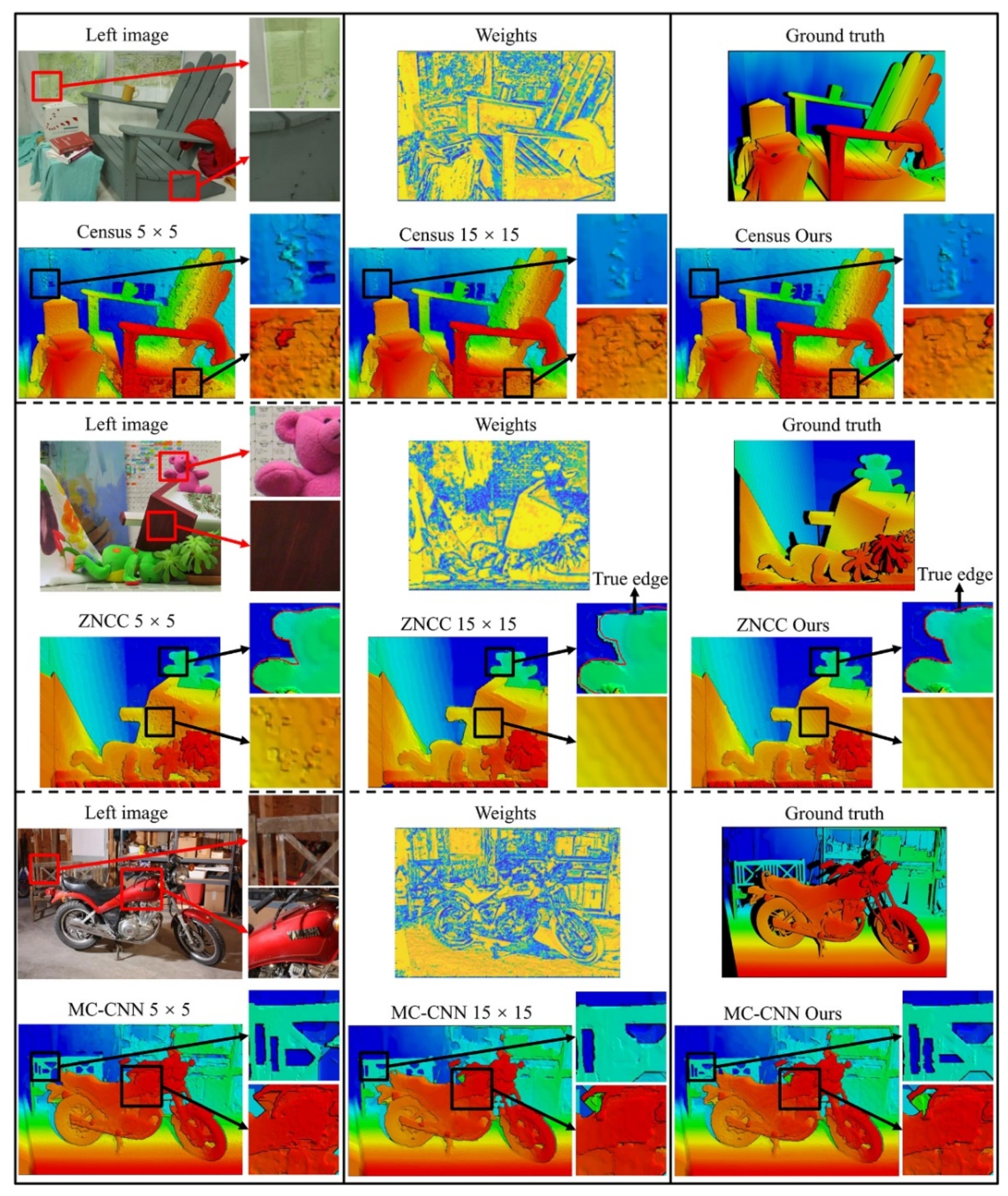
To visually illustrate the comparisons of our proposed method, 5 × 5 pixels matching window, and 15 × 15 pixels matching window, we select three representative stereo images in the Middlebury dataset, as shown in Figure 4.
The first image pair contained large weak-textured/untextured regions (e.g., the chair) and some repetitive textured regions (e.g., the left side of the map) where a 5 × 5 matching window produced serious mismatches, due to the high matching uncertainties in such regions, as shown in the left of the first row. A 15 × 15 matching window contained more image information such that they were able to compute more robust marching results in such regions, as shown in the middle of the first row. Our proposed method was able to achieve similar matching results to 15 × 15 pixels matching window, since most pixels in such regions tended to have higher weights of large windows.
In the second image pair, the disparity edges of 5 × 5 pixels were close to the image edges (the red lines in the second row of Figure 4), which shows that a 5 × 5 matching window is able to achieve high matching accuracies in edges (e.g., the edges of Teddy). However, it contained obvious mismatches in weak textured regions (e.g., the toy roof). Oppositely, a 15 × 15 matching window could be able to compute smooth surfaces in weak-textured regions (e.g., the toy roof). However, since the disparity consistency assumption cannot be satisfied in disparity jumps, it produces obvious mismatches in edges (e.g., the edges of Teddy). Our proposed method was capable of estimating higher weights of small windows in edges and higher weights of large windows in weak-textured regions, thus inheriting the advantages of both windows and computing the most accurate matching results. The matching results of both the 15 × 15 matching window and the proposed method in the lower sub-images have stair-like disparities. These stair-like disparities were caused by the penalization constraint of SGM, which penalized disparity jumps between adjacent pixels with similar intensity/color. Since the disparities in slanted or curved regions are not consistent, the penalization constraint of SGM will result in stair-like disparities, also termed as fronto-parallel biases [42].
The third image pair focus on testing the performance of the three methods on fine structures. The 5 × 5 pixels matching window, with our proposed method, was able to recover more precise details than the 15 × 15 pixels matching window. In general, our proposed method is able to leverage the advantages of both large and small windows and compute smooth, sharp disparity images in indoor datasets.

4.3. Experiment with the Aerial Dataset

To further evaluate the transferability of our proposed method, we tested our proposed method on two aerial stereo image pairs from Toronto, Canada, and Vaihingen, German. The Vaihingen data were provided by the German Society for Photogrammetry, Remote Sensing and Geoinformation (DGPF), and the Toronto data were provided by the city of Toronto, First Base Solutions, and York University’s GeoICT Lab. These two stereo image pairs are randomly selected from each of the Toronto and Vaihingen data because the scenarios in separate datasets are similar. Other tiles share similar characteristics. Random sampling can prove the reliability of our proposed method. True disparities of corresponding stereo pairs were generated by filtering inconsistent parts of LiDAR (Light Detection and Ranging) points (e.g., occlusions, temporal changes) in a dense matching framework (Huang et al. 2018) and then projecting the consistent LiDAR points onto epipolar space, thus generating true disparity images for the stereo pairs. Finally, we applied our proposed method, the 5 × 5 pixels matching window, the 15 × 15 pixels matching window, the 9 × 9 pixels matching window, the texture-based window selection method, the confidence-based window selection method, and our previous window size selection network (WSSN) method on the aerial dataset. We evaluated their average matching accuracies under bad pixel percentage strategies. To give a more comprehensive comparison between this work and our previous work [32], we also used the network in the previous work to compute the matching results with the appropriate matching windows. We evaluated its matching accuracy under the mismatch-3 metric, as shown in Table 2. The 5 × 5 pixels matching window still achieved the worst matching accuracies in the aerial image data. The texture-based window selection method also met the instability problem in different matching cost metrics, since it only considers the texture information. The matching accuracy of our work in this paper is slightly higher than our previous work in both the Census and ZNCC metrics since the new work considers more matching results through the fusion strategy and reduces the noises in the weight estimation results by imposing an energy function.
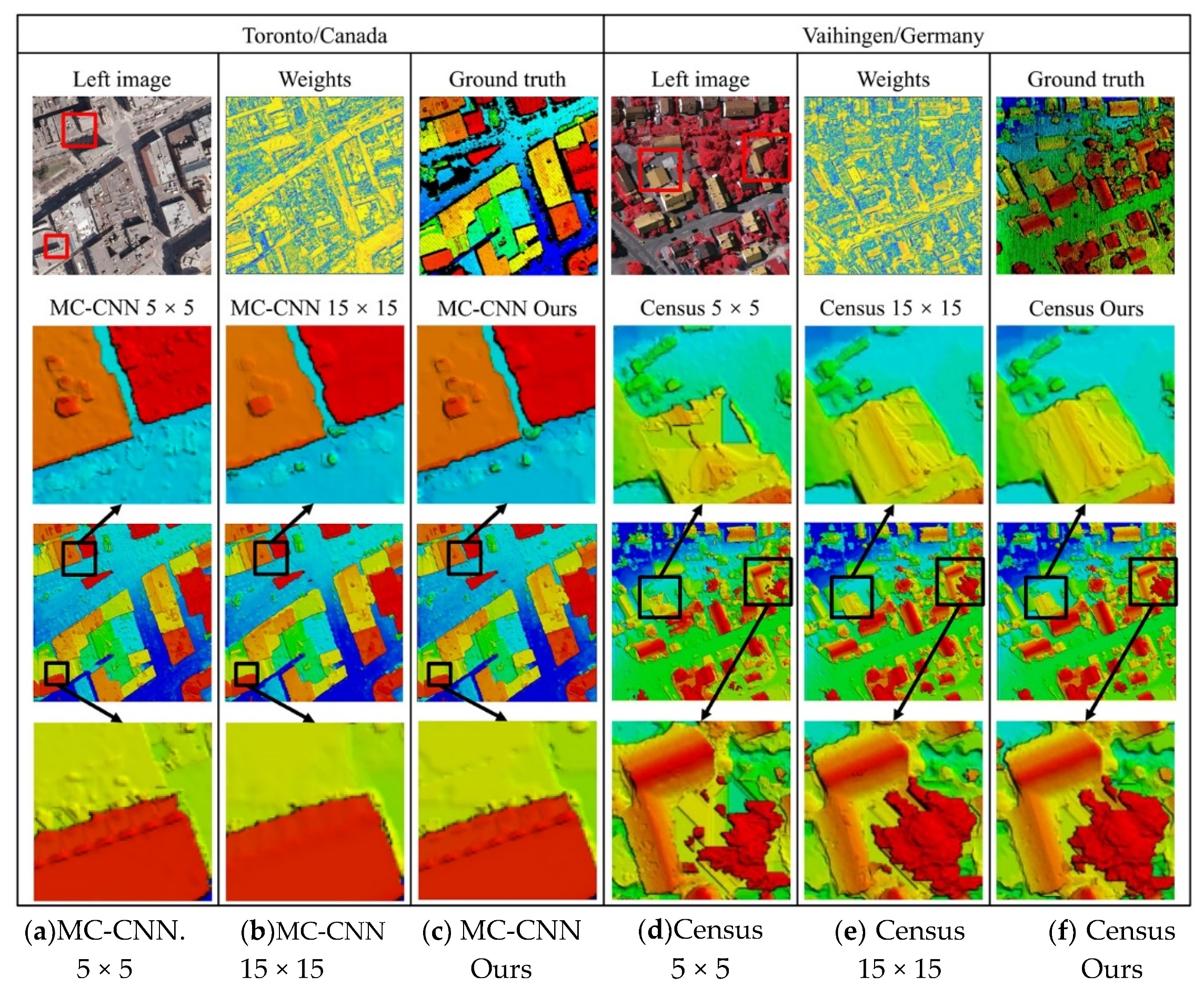
Since the scenarios in separate datasets are similar, we did our best to select regions of interest containing more corners, edges, fine structures, and sharp ridgelines of buildings with texture-less flat roofs, grounds, and gable roofs for better visual comparisons, as shown in Figure 5.
The Toronto image pair contained large weak-textured and repetitive textured regions (e.g., the flat roofs and ground) and untextured regions (e.g., the occlusion areas on the northwest of buildings), in which the 5 × 5 pixels matching window contained obvious mismatches, due to the high matching uncertainties in such regions, as shown in Figure 5a. The 15 × 15 pixels matching window took into account more image information such that it was able to achieve more robust marching results in such regions, of Figure 5b. Our proposed method in this paper was able to achieve similar smooth surfaces to the 15 × 15 pixels matching window on weak-textured and repetitive textured regions and details to the 5 × 5 pixels matching window on the fine-structure regions of the roofs.
The Vaihingen image pair mainly charactered with gable roofs and trees. The 5 × 5 pixels matching window is able to recover most edges of the buildings. However, it contained some mismatches in weak-textured regions, e.g., the roof and the tree area in Figure 5b. In contrast, the 15 × 15 pixels matching window can recover smooth surfaces in weak-textured regions. However, since the disparity consistency assumption cannot be satisfied in disparity jumps, it produces over-smooth edges (e.g., building boundary and the ridgelines of gable roofs). Our proposed method was capable of estimating higher weights of small windows in edges and higher weights of large windows in weak-textured regions, thus leveraging the advantages of both windows and computing the most accurate matching results.
It shows that the 5 × 5 pixels matching window was capable of recovering fine structures and sharp ridgelines of gable roofs (shown in Figure 5a), while it produced several mismatches on grounds and roof surfaces (e.g., Figure 5d). The 15 × 15 pixels matching window can compute smooth surfaces on grounds and roof surfaces (e.g., Figure 5e), while it would over smooth some details on the roofs (e.g., Figure 5b) since window-based methods have the underlying assumption that there are no disparities inconsistencies in a local window; thus, a large matching window will make the disparity inconsistency details over smooth. Our proposed method was able to compute smooth surfaces as well as keep details of fine structures, thus achieving the best matching accuracies.

4.4. Experiment with the Satellite Dataset

We assessed our proposed method on the satellite dataset on Jacksonville, FL, which was provided by Johns Hopkins University Applied Physics Laboratory (JHUAPL). The Jacksonville dataset included WorldView-3 images with the Ground Sampling Distance (GSD) as 0.3 m. We selected five stereo pairs in the Jacksonville dataset, and the corresponding true disparities were generated from LiDAR points. We compared our proposed method, the 5 × 5 pixels matching window, the 15 × 15 pixels matching window, the 9 × 9 pixels matching window, the texture-based window selection method, the confidence-based window selection method, and our previous window size selection network (WSSN) method on the satellite dataset. We evaluated their average matching accuracies as well as standard deviation ( σ ), range, and confidence interval under bad pixel percentage strategies, as shown in Table 3.
Table 3 lists the statistics of the bad pixel percentage for the five image pairs where, for each result, the statistical metrics are computed for (1) the 5 × 5 pixels window; (2) the 9 × 9 pixels window; (3) the 15 × 15 pixels window; (4) texture-based window selection [25]; (5) confidence-based window selection [31]; (6) window size selection network (WSSN) [32]; and (7) our proposed method. It can be seen from Table 3 for most of the seven matching window selection/fusion methods with the three matching cost metrics, 5 × 5 pixels matching window achieved the worst matching accuracies. Since satellite images had relatively low GSD, when compared with the indoor and the aerial dataset, the 5 × 5 pixels matching window is too small to contain enough image information, especially in some weak-textured regions (e.g., roads, roofs), thus resulting in high matching uncertainties (see the higher σ , ranges, and confidence intervals in Table 3). The 15 × 15 pixels matching window contained more image information in weak-textured regions, thus resulting in higher matching accuracies than the 5 × 5 pixels matching window (smaller means, σ , ranges, and confidence interval values in Table 3). The 9 × 9 pixels matching window is a trade-off between the 5 × 5 and 15 × 15 pixels matching windows. It is able to achieve similar matching accuracies to 15 × 15 pixels matching window in satellite dataset but less matching cost computation complexities. The texture-based window selection method achieved high matching accuracies on Census and MC-CNN-fst matching cost metrics, while low matching accuracies in ZNCC matching cost metrics, which shows the instability of such a method among different matching cost metrics. The confidence-based window selection method is only better than the 5 × 5 pixels matching window but worse than all other window selection strategies, which shows that the confidence-based method is unable to predict appropriate windows in satellite images, even though it considered both the texture and the disparity information. The Window size selection network (WSSN) method performs slightly better than other window selection methods in ZNCC matching cost metric. Finally, our proposed method achieved the best or comparable matching accuracies among all matching cost metrics. It shows that our proposed method can estimate appropriate window weights for the fusion of the matching results of each pixel in satellite images and achieve stable matching accuracies on different matching cost metrics. For a better understanding and comparison across different matching cost metrics of the distribution of mismatch-3 metric from each pair on the satellite dataset, we drew an improved boxplot based on eight numbers (minimum, standard deviation ( σ ), first quartile (Q1), median (second quartile, Q2), mean, third quartile (Q3), and maximum, as shown in the legend) in Figure 6. It can be seen from Figure 6 that our method also achieved the optimal interquartile range (IQR) for Census and the MC-CNN-fst matching cost metric, similar to the range and confidence interval shown in Table 3. The box bounds of the IQR is divided by the median. Comparing all the results on the three matching cost metrics, we proposed method achieved the smallest median, as shown in Figure 6.
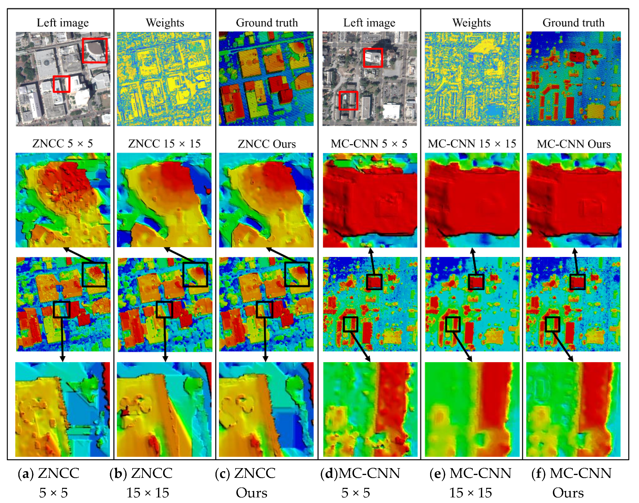
Figure 7 gives entire illustrations of matching results of the 5 × 5 pixels matching window, the 15 × 15 pixels matching window, and our proposed method on the first two stereo pairs. The weight map in Figure 7 shows the large and small window weights from our proposed method, where yellow shades mean higher large window weights, while blue shades mean higher small window weights. The 5 × 5 pixels matching window was able to recover details in most edges and strong textured regions (e.g., the last image in Figure 7a and the second image in Figure 7d), but such a small matching window is more likely to cause mismatches in weak textured regions (e.g., roofs of the second image in Figure 7a). The 15 × 15 pixels matching window was able to compute robust matching results in weak textured regions such as the roofs in the fifth image of the second row and the fifth image of the last row. However, such large windows always assume disparity consistency within the window, thus resulting in over smoothness in boundaries, as shown in the second image of the last row.
In the two-weight maps of the satellite dataset, the color of most pixels in roads and roofs were similar to yellow, which means that our proposed method tends to have higher large window weights in such weak-textured regions. In object boundaries (e.g., building boundaries), the color of most pixels is similar to blue, which means that our proposed method tends to have higher small window weights in disparity jumps. In general, our proposed method can estimate appropriate window weights of matching results fusion of each pixel, thus being able to combine the advantages of different size windows and overcome the disadvantages of the two windows to a certain extent to achieve the highest matching accuracy.

5. Conclusions

In this paper, we have proposed a novel adaptive window matching results fusion method to compute accurate disparity images with smooth surfaces and fine structures. We formulate the window selection/fusion problem as the minimization of a global energy function and propose a network structure to predict weights of large and small windows. We have further applied the proposed adaptive fusion method to compare with six other state-of-the-art matching window selection methods, including the 5 × 5 pixels matching window (small window), the 15 × 15 pixels matching window (large window), the 9 × 9 pixels matching window (middle window), the texture-based window selection method, the confidence-based window selection method, and our previous window size selection network method on the Middlebury dataset, the Toronto and Vaihingen aerial remote sensing dataset, and the Jacksonville satellite remote sensing dataset, aiming to achieve robust matching results in weak-textured regions and sharp boundaries and fine structures. The main contributions of our method include:
(1)
We have designed a neural network to predict window weights of matching results fusion of each pixel;
(2)
We have formulated the window selection problem as a global energy function so that some misestimation from the neural network could be refined;
(3)
A comprehensive quantitative assessment on the Middlebury dataset, the Toronto and Vaihingen aerial remote sensing dataset, and the Jacksonville satellite remote sensing dataset has been performed, with the comparative investigation with six other state-of-the-art matching window selection methods. The experimental results have shown that our proposed method achieved good transferability among different datasets.
In the experiments, we tested our proposed method on the above three datasets with three different matching cost metrics: Census, ZNCC, and MC-CNN-fst. The matching results of all methods have been optimized by Semi-Global Matching (SGM) and several post-processing steps (e.g., Winner-Takes-All (WTA), Left-Right Consistency (LRC), disparity interpolation) with the same matching parameters (e.g., penalty parameters in SGM). We evaluated the performances of our proposed method, the 5 × 5 pixels matching window, the 15 × 15 pixels matching window, the 9 × 9 pixels matching window, the texture-based window selection method, the confidence-based window selection method, and our previous window size selection network (WSSN) method by firstly finding bad pixels whose estimated disparities differ more than three pixels from its true disparities and then computing the percentage of bad pixels averaged over all ground truth pixels (termed as mismatch-3). A lower percentage means higher matching accuracies and vice versa. The experimental results of the Middlebury dataset, the Toronto and Vaihingen aerial remote sensing dataset, and the Jacksonville satellite remote sensing dataset demonstrated that our proposed method is able to compute robust disparities in weak-textured regions and accurate disparities in fine structures. As compared to the other six state-of-the-art matching window selection methods, our proposed method in this paper achieved the best matching accuracies with different matching cost metrics in all datasets.
Since the original version of MC-CNN-fst was trained using a 9 × 9 pixels window, the input images and the disparity range should be resized to generate the equivalent of different window sizes (i.e., 5 × 5 and 15 × 15) in our previous workflow. However, the processing of the resized images and disparity range exponentially increase the memory usage, which is beyond our current computational capacity. Therefore, we did not present the comparison with MC-CNN-fst for the WSSN method in this paper.
To further test our proposed adaptive window matching results fusion method to compute accurate disparity images in the future, we will consider adding more matching cost criteria, including classic low-level feature consistency measures and learning-based deep consistency measures for analysis and testing and improving our proposed method. The trained model and the AFC-CNN codes are made available to anyone interested in testing and improving our proposed method in the academic community upon request.

Author Contributions

All authors contributed to this paper. Y.H., W.L., and X.H. proposed the idea and processed the data, performed the experiment, and prepared the figures and tables. Y.H., W.L., and X.H. wrote the paper. S.W. oversaw the paper and the results and provided fruitful discussions. R.Q. oversaw the work, provided valuable comments and proofread the paper. Part of the work was performed while Y.H. was visiting The Ohio State University. All authors have read and agreed to the published version of the manuscript.

Funding

This research was supported by the Chinese Scholarship Council (grant number 201706270113) and the National Natural Science Foundation of China (grant number 41701540).

Acknowledgments

The authors would like to thank the German Society for Photogrammetry, Remote Sensing and Geoinformation (DGPF) for providing the Vaihingen dataset, and the Optech Inc., First Base Solutions Inc., York University, and ISPRS WG III/4 for providing the Downtown Toronto dataset. The authors also would like to thank the Johns Hopkins University Applied Physics Laboratory and IARPA for providing the data used in this study, and the IEEE GRSS Image Analysis and Data Fusion Technical Committee for organizing the Data Fusion Contest.

Conflicts of Interest

The authors declare no conflict of interest.

References

  1. Hirschmüller, H.; Scharstein, D. Evaluation of stereo matching costs on images with radiometric differences. IEEE Trans. Pattern Anal. Mach. Intell. 2009, 31, 1582–1599. [Google Scholar] [CrossRef]
  2. Yuan, W.; Yuan, X.; Xu, S.; Gong, J.; Shibasaki, R. Dense image-matching via optical flow field estimation and fast-guided filter refinement. Remote Sens. 2019, 11, 2410. [Google Scholar] [CrossRef] [Green Version]
  3. Ye, Z.; Xu, Y.; Chen, H.; Zhu, J.; Tong, X.; Stilla, U. Area-Based dense image matching with subpixel accuracy for remote sensing applications: Practical analysis and comparative study. Remote Sens. 2020, 12, 696. [Google Scholar] [CrossRef] [Green Version]
  4. Nebiker, S.; Lack, N.; Deuber, M. Building change detection from historical aerial photographs using dense image matching and object-based image analysis. Remote Sens. 2014, 6, 8310–8336. [Google Scholar] [CrossRef] [Green Version]
  5. Bergamasco, F.; Torsello, A.; Sclavo, M.; Barbariol, F.; Benetazzo, A. WASS: An open-source pipeline for 3D stereo reconstruction of ocean waves. Comput. Geosci. 2017, 107, 28–36. [Google Scholar] [CrossRef]
  6. Han, Y.; Qin, R.; Huang, X. Assessment of dense image matchers for digital surface model generation using airborne and spaceborne images–an update. Photogramm. Rec. 2020, 35, 58–80. [Google Scholar] [CrossRef]
  7. Remondino, F.; Spera, M.G.; Nocerino, E.; Menna, F.; Nex, F. State of the art in high density image matching. Photogramm. Rec. 2014, 29, 144–166. [Google Scholar] [CrossRef] [Green Version]
  8. Zhang, W.; Zhang, X.; Chen, Y.; Yan, K.; Yan, G.; Liu, Q.; Zhou, G. Generation of pixel-level resolution lunar DEM based on Chang’E-1 three-line imagery and laser altimeter data. Comput. Geosci. 2013, 59, 53–59. [Google Scholar] [CrossRef]
  9. Han, Y.; Wang, S.; Gong, D.; Wang, Y.; Wang, Y.; Ma, X. State of the art in digital surface modelling from multi-view high-resolution satellite images. ISPRS Ann. Photogramm. Remote Sens. Spat. Inf. Sci. 2020, 2, 351–356. [Google Scholar] [CrossRef]
  10. Scharstein, D.; Szeliski, R. A taxonomy and evaluation of dense two-frame stereo correspondence algorithms. Int. J. Comput. Vis. 2002, 47, 7–42. [Google Scholar] [CrossRef]
  11. Birchfield, S.; Tomasi, C. A pixel dissimilarity measure that is insensitive to image sampling. IEEE Trans. Pattern Anal. Mach. Intell. 1998, 20, 401–406. [Google Scholar] [CrossRef] [Green Version]
  12. Mei, X.; Sun, X.; Zhou, M.; Jiao, S.; Wang, H.; Zhang, X. On building an accurate stereo matching system on graphics hardware. In Proceedings of the 2011 IEEE International Conference on Computer Vision Workshops (ICCV Workshops), Barcelona, Spain, 6–13 November 2011; pp. 467–474. [Google Scholar] [CrossRef]
  13. Hermann, S.; Vaudrey, T. The gradient-a powerful and robust cost function for stereo matching. In Proceedings of the 2010 25th International Conference of Image and Vision Computing New Zealand, Queenstown, New Zealand, 8–9 November 2010; pp. 1–8. [Google Scholar] [CrossRef]
  14. Huang, X.; Zhang, Y.; Yue, Z. Image-guided non-local dense matching with three-steps optimization. ISPRS Ann. Photogramm. Remote Sens. Spat. Inf. Sci. 2016, III-3, 67–74. [Google Scholar] [CrossRef]
  15. Zhou, X.; Boulanger, P. Radiometric invariant stereo matching based on relative gradients. In Proceedings of the 2012 19th IEEE International Conference on Image Processing, Orlando, FL, USA, 30 September–3 October 2012; pp. 2989–2992. [Google Scholar] [CrossRef]
  16. Mozerov, M.G.; van de Weijer, J. Accurate stereo matching by two-step energy minimization. IEEE Trans. Image Process. 2015, 24, 1153–1163. [Google Scholar] [CrossRef] [PubMed]
  17. Zabih, R.; Woodfill, J. Non-parametric local transforms for computing visual correspondence. In Proceedings of the European Conference on Computer Vision, Stockholm, Sweden, 2–6 May 1994; pp. 151–158. [Google Scholar] [CrossRef] [Green Version]
  18. Jung, I.-L.; Chung, T.-Y.; Sim, J.-Y.; Kim, C.-S. Consistent stereo matching under varying radiometric conditions. IEEE Trans. MultiMedia 2012, 15, 56–69. [Google Scholar] [CrossRef]
  19. Jiao, J.; Wang, R.; Wang, W.; Dong, S.; Wang, Z.; Gao, W. Local stereo matching with improved matching cost and disparity refinement. IEEE MultiMedia 2014, 21, 16–27. [Google Scholar] [CrossRef]
  20. Kordelas, G.A.; Alexiadis, D.S.; Daras, P.; Izquierdo, E. Enhanced disparity estimation in stereo images. Image Vis. Comput. 2015, 35, 31–49. [Google Scholar] [CrossRef]
  21. Li, Y.; Zheng, S.; Wang, X.; Ma, H. An efficient photogrammetric stereo matching method for high-resolution images. Comput. Geosci. 2016, 97, 58–66. [Google Scholar] [CrossRef]
  22. Zbontar, J.; LeCun, Y. Stereo Matching by Training a Convolutional Neural Network to Compare Image Patches. J. Mach. Learn. Res. 2016, 17, 2. [Google Scholar]
  23. Hirschmüller, H. Stereo Processing by Semiglobal Matching and Mutual Information. IEEE Trans. Pattern Anal. Mach. Intell. 2008, 30, 328–341. [Google Scholar] [CrossRef]
  24. Erway, C.C.; Ransford, B. Variable Window Methods for Stereo Disparity Determination. Machine Vision 2017. [Google Scholar] [CrossRef]
  25. Lin, P.-H.; Yeh, J.-S.; Wu, F.-C.; Chuang, Y.-Y. Depth estimation for lytro images by adaptive window matching on EPI. J. Imaging 2017, 3, 17. [Google Scholar] [CrossRef] [Green Version]
  26. Emlek, A.; Peker, M.; Dilaver, K.F. Variable window size for stereo image matching based on edge information. In Proceedings of the 2017 International Artificial Intelligence and Data Processing Symposium (IDAP), Malatya, Turkey, 16–17 September 2017; pp. 1–4. [Google Scholar] [CrossRef]
  27. Koo, H.-S.; Jeong, C.-S. An area-based stereo matching using adaptive search range and window size. In Proceedings of the International Conference on Computational Science, San Francisco, USA, 28–30 May 2001; pp. 44–53. [Google Scholar] [CrossRef] [Green Version]
  28. Debella-Gilo, M.; Kääb, A. Locally adaptive template sizes for matching repeat images of Earth surface mass movements. ISPRS J. Photogramm. Remote Sens. 2012, 69, 10–28. [Google Scholar] [CrossRef]
  29. He, Y.; Wang, P.; Fu, J. An Adaptive Window Stereo Matching Based on Gradient. In Proceedings of the 3rd International Conference on Electric and Electronics, Hong Kong, China, 24–25 December 2013. [Google Scholar] [CrossRef] [Green Version]
  30. Kanade, T.; Okutomi, M. A stereo matching algorithm with an adaptive window: Theory and experiment. IEEE Trans. Pattern Anal. Mach. Intell. 1994, 16, 920–932. [Google Scholar] [CrossRef] [Green Version]
  31. Adhyapak, S.; Kehtarnavaz, N.; Nadin, M. Stereo matching via selective multiple windows. J. Electron. Imaging 2007, 16, 013012. [Google Scholar] [CrossRef] [Green Version]
  32. Huang, X.; Liu, W.; Qin, R. A window size selection network for stereo dense image matching. Int. J. Remote Sens. 2020, 41, 4838–4848. [Google Scholar] [CrossRef]
  33. Hirschmüller, H. Accurate and efficient stereo processing by semi-global matching and mutual information. In Proceedings of the 2005 IEEE Computer Society Conference on Computer Vision and Pattern Recognition (CVPR’05), San Diego, CA, USA, 20–25 June 2005; pp. 807–814. [Google Scholar] [CrossRef]
  34. Geiger, A.; Lenz, P.; Stiller, C.; Urtasun, R. Vision meets robotics: The KITTI dataset. Int. J. Robot. Res. 2013, 32, 1231–1237. [Google Scholar] [CrossRef] [Green Version]
  35. Di Stefano, L.; Mattoccia, S.; Tombari, F. ZNCC-based template matching using bounded partial correlation. Pattern Recognit. Lett. 2005, 26, 2129–2134. [Google Scholar] [CrossRef]
  36. Cheng, F.; Zhang, H.; Sun, M.; Yuan, D. Cross-trees, edge and superpixel priors-based cost aggregation for stereo matching. Pattern Recognit. 2015, 48, 2269–2278. [Google Scholar] [CrossRef] [Green Version]
  37. Taniai, T.; Matsushita, Y.; Naemura, T. Graph cut based continuous stereo matching using locally shared labels. In Proceedings of the IEEE Conference on Computer Vision and Pattern Recognition, Columbus, OH, USA, 23–28 June 2014; pp. 1613–1620. [Google Scholar] [CrossRef]
  38. Scharstein, D.; Hirschmüller, H.; Kitajima, Y.; Krathwohl, G.; Nešić, N.; Wang, X.; Westling, P. High-resolution stereo datasets with subpixel-accurate ground truth. In Proceedings of the German conference on pattern recognition, Münster, Germany, 2–5 September 2014; pp. 31–42. [Google Scholar] [CrossRef] [Green Version]
  39. Rottensteiner, F.; Sohn, G.; Jung, J.; Gerke, M.; Baillard, C.; Benitez, S.; Breitkopf, U. The ISPRS benchmark on urban object classification and 3D building reconstruction. ISPRS Ann. Photogramm. Remote Sens. Spat. Inf. Sci 2012, 1, 293–298. [Google Scholar] [CrossRef] [Green Version]
  40. Bosch, M.; Foster, K.; Christie, G.; Wang, S.; Hager, G.D.; Brown, M. Semantic stereo for incidental satellite images. In Proceedings of the 2019 IEEE Winter Conference on Applications of Computer Vision (WACV), Waikoloa, HI, USA, 7–11 January 2019; pp. 1524–1532. [Google Scholar] [CrossRef] [Green Version]
  41. Saux, B.L.; Yokoya, N.; Hänsch, R.; Brown, M. Data Fusion Contest 2019 (DFC2019). Available online: https://ieee-dataport.org/open-access/data-fusion-contest-2019-dfc2019 (accessed on 7 June 2020).
  42. Olsson, C.; Ulén, J.; Boykov, Y. In defense of 3d-label stereo. In Proceedings of the IEEE Conference on Computer Vision and Pattern Recognition, Portland, OR, USA, 23–28 June 2013; pp. 1730–1737. [Google Scholar] [CrossRef]
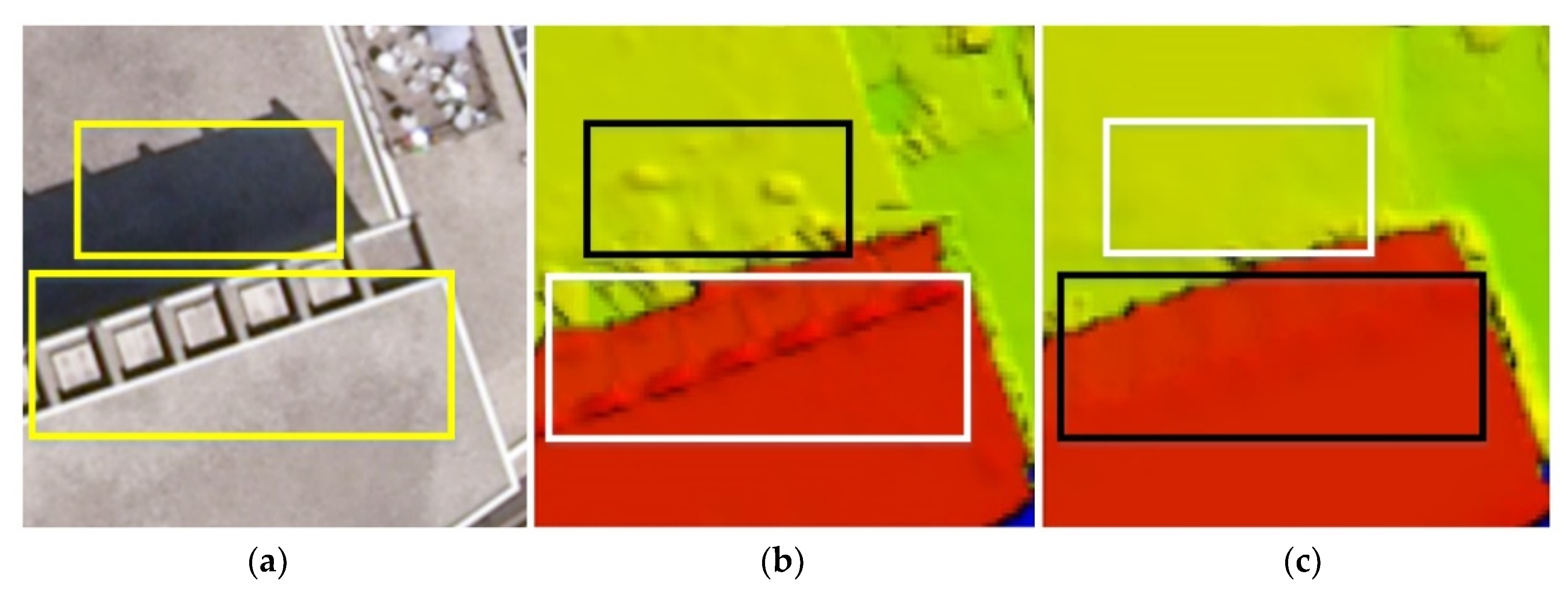
Figure 1. Comparison between the matching results using small and large windows: (a) the original image; (b) the matching result in 5 × 5 pixels window; (c) the matching result in 15 × 15 pixels window. Both (b) and (c) are estimated disparity images using Census-based Hamming distance as the matching cost [17,22] with semi-global matching optimization [23].
Remotesensing 12 03138 g001
Figure 2. Overview of our work: ① shows the input of our workflow; the aggregated matching cost volumes are computed from Semi-Global Matching (SGM), and then an initial disparity image is derived from the aggregated matching cost volumes of small matching windows. ② shows the estimated weight maps of small windows and large windows. ③ is a process to refine weight maps. ④ shows the fused matching cost volume by weighted averaging the aggregated cost volumes of small and large windows. ⑤ is post-processing that includes Winner-Takes-All (WTA), Left-Right Consistency (LRC), and disparity interpolation. ⑥ shows the final disparity image using the proposed method.
Remotesensing 12 03138 g002
Figure 3. Proposed Adaptive Matching Fusion based on Convolutional Neural Network (AMF-CNN) structure.
Remotesensing 12 03138 g003
Figure 4. Examples of disparity images on the Middlebury dataset.
Remotesensing 12 03138 g004
Figure 5. Examples of disparity images on the aerial dataset.
Remotesensing 12 03138 g005
Figure 6. Boxplot of statistics from the mismatch-3 on the satellite dataset.
Remotesensing 12 03138 g006
Figure 7. Examples of disparity images on the satellite dataset.
Remotesensing 12 03138 g007
Table 1. Mismatch-3 comparison of seven different methods on the Middlebury dataset (bold records indicate the top-three optimal results among each of the considered matching cost metrics).
MethodCensusZNCCMC-CNN-fst
5 × 5 pixels0.15200.16720.1183
9 × 9 pixels0.13720.15250.1092
15 × 15 pixels0.13310.16110.1136
Texture-based window selection [25]0.12470.17290.1403
Confidence-based window selection [31]0.12860.15620.1146
Window size selection network (WSSN) [32]0.12430.1497\
Ours0.12300.14910.1038
Table 2. Mismatch-3 comparison of seven different methods on the aerial dataset (bold records indicate the top-three optimal results among each of the considered matching cost metrics).
MethodCensusZNCCMC-CNN-fst
5 × 5 pixels0.14930.15230.1127
9 × 9 pixels0.12810.13280.1103
15 × 15 pixels0.12150.14080.1134
Texture-based window selection [25]0.12180.13340.1147
Confidence-based window selection [31]0.12000.13920.1137
Window size selection network (WSSN) [32]0.11440.1345\
Ours0.11190.12320.0969
Table 3. Mismatch-3 comparison of seven different methods on the satellite dataset (bold records indicate the top-three optimal results among each of the considered statistical/matching cost metrics).
Method CensusZNCCMC-CNN-fst
5 × 5 pixelsmean0.15200.15940.1415
σ 0.06710.07160.0658
range0.16740.17620.1607
Confidence interval(0.0932,0.2108)(0.0966,0.2222)(0.0838,0.1992)
9 × 9 pixelsmean0.13730.14230.1287
σ 0.06270.06950.0624
range0.16380.17290.1527
Confidence interval(0.0824,0.1923)(0.0813,0.2032)(0.0740,0.1834)
15 × 15 pixelsmean0.13020.14520.1258
σ 0.06100.07100.0629
range0.15660.17970.1535
Confidence interval(0.0767,0.1837)(0.0830,0.2075)(0.0707,0.1809)
Texture-based window selection [25]mean0.13020.14640.1253
σ 0.06150.07410.0619
range0.15700.18600.1504
Confidence interval(0.0764,0.1841)(0.0815,0.2115)(0.0711,0.1796)
Confidence-based window selection [31]mean0.14290.14520.1344
σ 0.06370.06990.0640
range0.16330.17130.1599
Confidence interval(0.0871,0.1987)(0.0840,0.2065)(0.0783,0.1905)
Window size selection network (WSSN) [32]mean0.13120.1420\
σ 0.06190.0717
range0.15650.1833
Confidence interval(0.0769,0.1855)(0.0795,0.2052)
Oursmean0.12980.14380.1208
σ 0.06120.07310.0599
range0.15700.18670.1492
Confidence interval(0.0762,0.1835)(0.0797,0.2078)(0.0684,0.1733)