Article

Joint Inversion of Geodetic Observations and Relative Weighting—The 1999 Mw 7.6 Chi-Chi Earthquake Revisited

1
Newcastle University, School of Engineering, Newcastle Upon Tyne NE1 7RU, UK
2
COMET, School of Engineering, Newcastle University, Newcastle upon Tyne NE1 7RU, UK
3
Department of Geosciences, National Taiwan University, Taipei 10617, Taiwan
4
Guangdong Provincial Key Laboratory of Geodynamics and Geohazards, School of Earth Sciences and Engineering, Sun Yat-Sen University, Guangzhou 510275, China
5
Southern Marine Science and Engineering Guangdong Laboratory (Zhuhai), Zhuhai 519082, China
6
Key Laboratory of Comprehensive and Highly Efficient Utilization of Salt Lake Resources, Qinghai Institution of Salt Lakes, Chinese Academy of Sciences, Xining 810008, China
*
Author to whom correspondence should be addressed.
Remote Sens. 2020, 12(19), 3125; https://doi.org/10.3390/rs12193125
Submission received: 10 August 2020 / Revised: 3 September 2020 / Accepted: 19 September 2020 / Published: 23 September 2020

Abstract

:
The M w 7.6 Chi-Chi earthquake struck central western Taiwan in 1999. The rupture was complex with several dislocations along the 100-km long Chelungpu thrust fault. Revisiting this earthquake is a challenge, as the precision and coverage of the data sets available are quite poor. Furthermore, the topographic and vegetation coverage complexity of the area prevents coherent radar images. In this paper, radar and optical images, and terrestrial geodetic measurements, were utilised to study the fault. The Particle Swarm Optimization and Okada Inversion (PSOKINV) geodetic inversion package was used with the generalized Akaike’s Bayesian Information Criterion (gABIC) to precisely determine the slip distribution and relative weighting of datasets. Differences in results using the data sets jointly or separately (e.g., under-estimation due to InSAR, inconsistencies in SPOT offsets, smoother slip distribution with gABIC weighting) are observable. Most of the energy was released in the northern part of the fault, where the strike veers toward the east, and mainly at depths less than 4 km. The PSOKINV-gABIC approach is viable for the study of complicated cases such as the Chi-Chi earthquake and can significantly benefit the weight determination and physical realism of the fault geometry.

Graphical Abstract

1. Introduction

Taiwan is the emerged part of an orogen formed by the collision between the Eurasian and Philippine Sea plates [1] entering in convergence at a rate of 82 mm/year with an orientation of 310 ° . Two subductions are consuming the island—at the south, the Eurasian plate goes beneath the Philippine sea plate in the east direction at the Manila trench, and the Philippine sea plate subducts towards the north near the Ryukyu trench. It is a high-risk seismic area (Figure 1) with the major and most destructive inland earthquake of the 20th century being the Chi-Chi event in central western Taiwan, occurring on 21st September 1999 with a magnitude of M w 7.6 and at a depth of 33 km (according to United States Geological Survey (USGS)). The seismic moment is estimated at 3.046 × 10 20 N · m by the USGS with a mean slip of 2–3 m . Thousands of people were injured or killed, and many infrastructures were destroyed. During the three months following the event [2], thousands of aftershocks occurred including six with a magnitude greater than 6.5, starting at the north and migrating downward and southward of the main event [3]. As presented in Reference [4], it is interesting to look at the seismicity (Figure 1) and its implications for the tectonics—two NW-SE patterns, one starting at the north of the fault and one at the south end between the Luliao and Tachienshan faults are clearly visible and point out the impact of this event on nearby faults such as the Luliao fault that most probably was activated during the Chi-Chi event. This earthquake was due to the reactivation of the Chelungpu fault: thrust faulting on a north-south striking fault plane dipping to the east [5]. The rupture was complex with several dislocations; it reached the surface and created a 100 km-long scarp between the hanging-wall to the east and the footwall to the west [6]. From GPS data (Figure 1), a clear change of surface motion is visible at the north end of the fault turning toward east. According to the focal mechanism, this event is in agreement with the SE-NW plate convergence motion [7], with an overlap toward west linked to the orogen deformation and a double plate convergence boundary, on each side of the central range [8].
Over the past 20 years, several models of the Chi-Chi earthquake were computed, each of them focusing on specific aspects, using different data sets, techniques and/or methods. For instance, Reference [2] showed by using seismological data that the total rupture duration is 28 s starting at the south of the fault and a northward propagation with static offset up to 8 s , mainly at shallow depths of less than 10 km . The GPS measurements acquired from three years before the event to a few months after [9] showed major horizontal displacements of 1.1 m to 9.1 m from NW to NNW on the hanging-wall with an uplift of 1.2 m to 4.4 m near the rupture. The deformation is less significant towards the east and increases near the end north of the fault. Regarding the footwall, 0.1 m to 1.5 m were detected toward SE to ESE for horizontal displacements and 0.02 m to 0.26 m of subsidence.
Regarding studies using InSAR, only the ERS (European Remote-Sensing Satellite) constellation was previously used. Reference [6] used ERS-2 products combined with GPS to study the footwall and reported some issues—the existence of a linear trend in phase difference caused by orbital error and atmospheric effects, also the presence of non-coseismic displacements. Linear trend correction using GPS was applied to the interferograms to remove large scale perturbations but GPS are too sparse to constrain the error; 1.7 cm of uncertainty is estimated on the centimeter accuracy coseismic displacement map [6].
Due to limited contributions from ERS-2 interferometry to the surface coseismic deformation mapping of the hanging-wall, area presenting the major deformation but covered by a dense vegetation, a few researchers turned to optical images. Reference [10] used SPOT (Satellite Pour l’Observation de la Terre) images and interpreted the coseismic slip as shallow and detected more displacement on the hanging-wall than the footwall. Also, they estimated that the deeper part of the fault was not activated during the event and the western front of the area should produce a M w 7 to 7.5 event every 150–250 years. Reference [11] used aerial photos which gave understanding of the hanging-wall to build a high-resolution map of the horizontal coseismic deformation. However, Reference [6] pointed out that non-negligible residuals were presented in Reference [10] and Reference [12] GPS based models. The residuals between each model and InSAR observations are estimated at 17 cm for Reference [10] and 7 cm for Reference [12]. One explanation for this difference is the geometry used: Reference [12] uses a point source method while Reference [10] uses a plane dislocation [13].
Mainly based on GPS but also combining data sets (InSAR, SPOT or Aerial photos), a few models were designed. Reference [14] built a four segment model based on GPS including a ramp decollement system at depth with a lateral ramp at the northern end. The main part is of about 70 km from the south to the north from Chushan to Fengyun, then an 8 km long segment bending to the east and finally a 25 km segment trending up to Shuangchi. Using GPS and InSAR, Reference [15] constructed a model with triangular elements, a more realistic dislocation method to represent the curved three-dimensional fault surface without introducing overlaps and gaps. It shows similar slip pattern to GPS based models, but the magnitude of the fault slip is smaller and the slip pattern smoother.
The results of Reference [10] based on SPOT imagery pointed out a shallow 20–35 ° east dipping ramp with a low dipping decollement at a depth of 6 to 8 km . However, a more recent paper, Reference [16], concluded a decollement at a depth of about 12 km , more consistent with the hypocentral depth of the mainshock and the distribution of aftershocks. According to them, the maximum slip is between 10 and 15 km on the shallow northern part of the fault with a moment of 3.6 × 10 20 N · m but most of the moment was released at shallow depths (between 0 and 5 km). In addition, the area ruptured by the main shock was fully locked before the earthquake. The slip is mainly aseismic for depths above 10 km [16]. No earthquake similar in magnitude to Chi-Chi’s is known to have occurred in recent centuries in central western Taiwan.
In this study, we use five types (Figure 1) of geodetic observations (GPS, levelling, benchmarks of urban planning, InSAR and SPOT offsets) in a joint inversion in order to estimate the slip distribution with and without precise estimation of the relative weights. In previous models, non-negligible residuals are present due to lack of information (density of the GPS network and no coherence on the hanging-wall for InSAR). This study focuses on showing the importance of combining and using complementary data sets rather than improving the model geometry. The fault geometry was determined by previous studies and slightly modified as a result of our data. The method presented in this paper shows the impact of the different data sets on the slip distribution as well as the necessity to properly determine the relative weights.

2. Geodetic Data Sets and Processing

The use of geodetic observation data is efficient for the study of earthquakes because of their high precision and their complementarity. In this study, several types have been selected—GPS, ERS-SAR and SPOT-optical images, levelling and benchmarks. GPS data have a high temporal resolution and a precision less than 1 mm/year useful to study slow deformation such as the post-seismic phase but it can also be used to study fast deformation such as the co-seismic phase; however their spatial distribution is sparse. Levelling and benchmarks have also an high spatial precision (few cm or higher) but rely on field measurement campaigns. InSAR data have a high spatial density and sub-cm precision but a low temporal sampling rate depending on the satellite (for instance, 6 days for Sentinel satellites but 35 days for ERS). Finally, SPOT images have a similar spatial density to SAR images, but can often provide useful measurements despite vegetation where SAR images lose coherence and at higher density than a pixel offset map estimated from the SAR amplitude would give. Even though the study area is partially covered by dense vegetation making InSAR output non-coherent, the joint study of InSAR with correlation of optical images and terrestrial measurements is an efficient and precise way to understand earthquakes. In central western Taiwan, from InSAR outputs, information about the footwall of the fault is obtained and SPOT offsets cover the full study area more densely than GPS. Levelling and benchmarks give precision about vertical movements and about the curved part at the north of the fault as benchmarks were measured only in this area (Figure 1B,C).

2.1. GPS Measurements
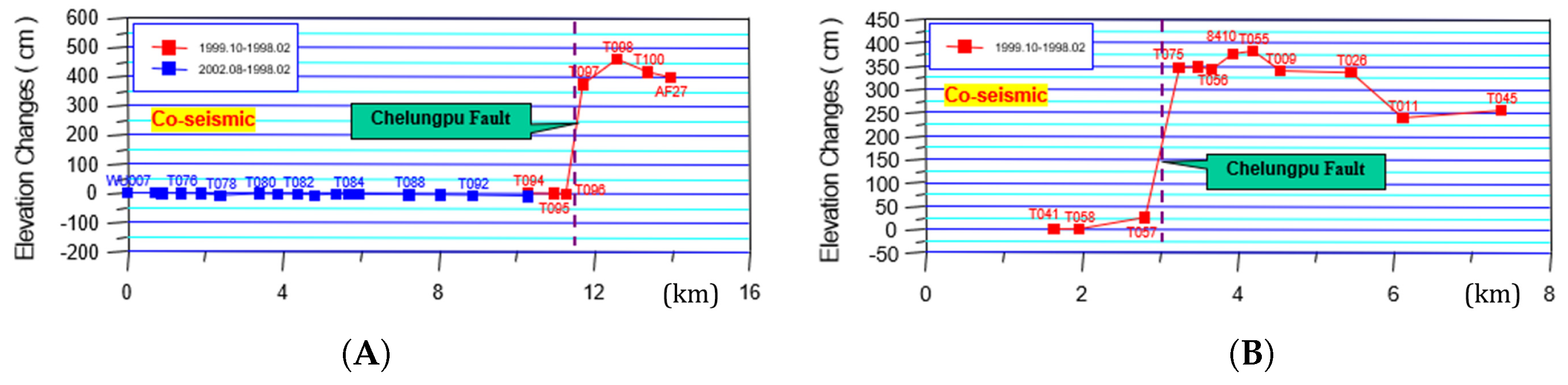
The GPS network in Taiwan was installed in 1989 and has been surveyed since 1990 covering the whole island. Figure 2 is showing benchmarks and an antenna of the Taiwan network. Specifically for the coseismic study (Figure 1A), the displacements were extracted from Reference [9]. 41 permanent stations are available (operated by the Central Weather Bureau (CWB); the Satellite Survey Division and Land Survey Bureau, Ministry of Interior (MOI) and the Institute of Earth Sciences, Academia Sinica (IESAS)) and 101 campaign-surveyed stations (conducted by three institutions (the Central Geological Survey, Ministry of Economic Affairs (MOEA, CGS); MOI and IESAS)) covering 1992 to 1999. They separated pre- and post-seismic deformation to estimate the coseismic displacement due to the Chi-Chi earthquake. They were processed using Bernese software v. 4.0 and corrected with precise ephemerides, and residual tropospheric zenith delays were estimated by least squares. The reference station selected is Kinmen, located on the east coast of mainland China (∼257 km from the epicenter) which did not show any coseismic movement. Furthermore, the pre-seismic secular motions were corrected by interpolating the velocity of 24 stations observed from 1992 to 1999. Finally, post-seismic displacements were corrected at the stations surveyed during the three months following the earthquake by interpolation from the nearby stations [17]. GPS, benchmarks and levelling are well correlated with each other.
In addition to GPS data, benchmarks of urban planning [18] situated at the north part of the fault, in Fengyuan city, were used (locations shown by the purple dashed box in Figure 1A and the displacements on the footwall and hanging wall in Figure 1B,C respectively). The pre-earthquake benchmarks were measured by total-station and the survey after the earthquake is a mixture of total station trilateration/triangulation and GPS campaigns. The horizontal positions were estimated by total station trilateration/triangulation. The data were provided with respect to the origin of TWD67 System (Transverse Mercator Two-degree Grid system) that we converted to WGS84 (World Geodetic System 1984) to be consistent with the rest of the data sets. The densely spaced distribution of the city-planning benchmarks provides an accurate location of constructions. Before the earthquake, a city map was created giving accurate position of human constructions. As many constructions were damaged during the earthquake, a second survey was run to remap the city after the event, the new map contains all the old city-planning benchmarks as well as Chi-Chi earthquake surface ruptures. The coseismic horizontal displacement data set was extracted from the comparison of these two maps. The horizontal displacements present an uncertainty of 1–2 cm against a mean displacement of 5 m in this area for the coseismic displacements.

2.2. Levelling Data

In addition to GPS data, levelling measurements (locations shown by the dark-blue dashed box in Figure 1A and the displacements in Figure 1D) were procured by CGS (MOEA) from 1998 to 2002 and converted from TWD67 to WGS84. They give more information about the vertical displacement, and are consistent with the GPS. Two of the six levelling lines are presented in Figure 3.

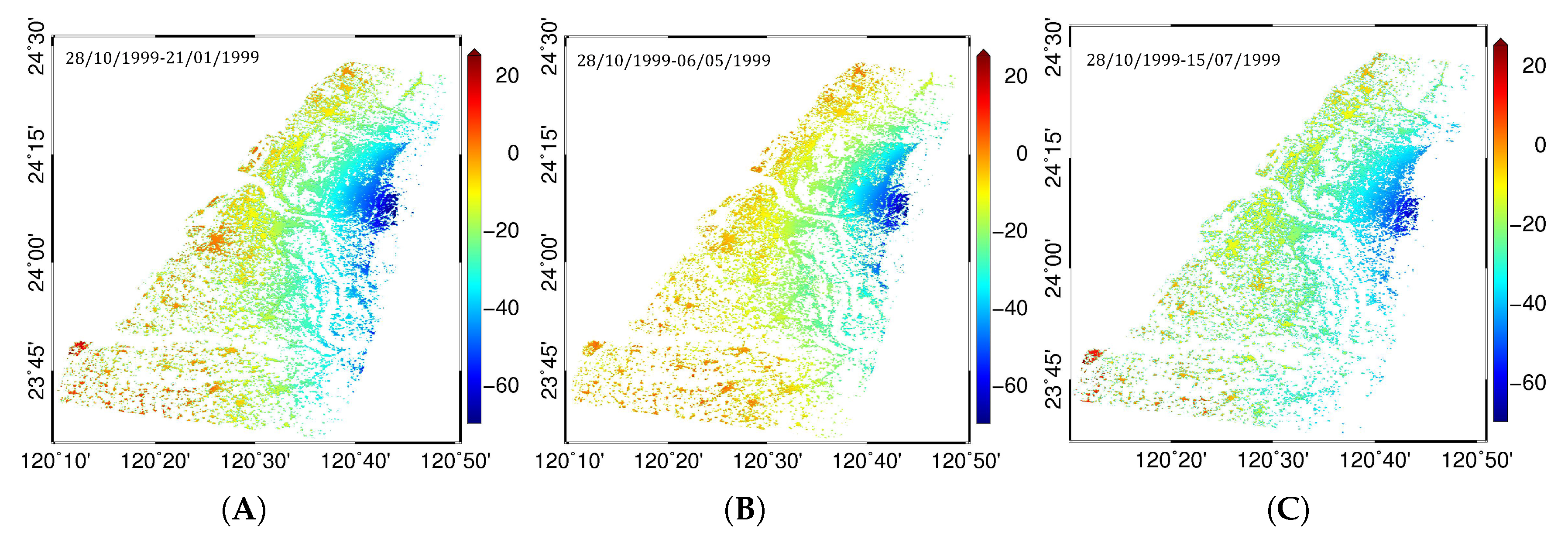
2.3. InSAR: ERS-2 Interferometric Processing Chain

ERS images were interferometrically processed using the ESA (European Space Agency) open-software SNAP (Sentinel Application Platform). Their parameters are presented in Table 1 and their coverage shown in Figure 1A. Only the footwall of the fault could be analyzed on the interferograms. The hanging-wall, which experienced the main deformation during this event, is densely vegetated resulting in low coherence. Coseismic interferograms show about 10–11 fringes in the footwall which is equivalent to a surface displacement of up to 30 cm (Figure 4).
Three interferograms were processed using SNAP and SNAPHU (Statistical-cost, Network-flow Algorithm for Phase Unwrapping [19,20,21]) for unwrapping the phase (the interferograms are consistent to each other with a regression coefficient of 0.7–0.8). After the coregistration of the primary and secondary images using Delft orbits and a 30 m SRTM (Shuttle Radar Topography Mission) DEM (Digital Elevation Model), the interferograms were formed and multilooked by 4 × 20 pixels to reduce the speckle effect, which gives a ground resolution of about 80 m. Finally, the interferograms were corrected for the effects of topography using the 1 arc-second (30 m) resolution SRTM DEM and filtered using Goldstein filtering (an adaptative power spectrum filter [22]) before unwrapping the phase and geocoding. Only pixels with a coherence higher than 0.2 were kept to be used in the joint inversion. The low coherence was the main challenge of the InSAR processing especially for the unwrapping of the phase. Furthermore, the hanging-wall of the fault, which is covered by dense vegetation, presents the main deformation as shown by GPS data. Thus, the main area of the deformation is not visible on the interferograms. Due to this reason, we decided to use optical images in addition to the radar interferometry. They have a better spatial resolution (10 m) than pixel offsets from InSAR (about 20 m) and will give us information about the deformation on both sides of the fault.

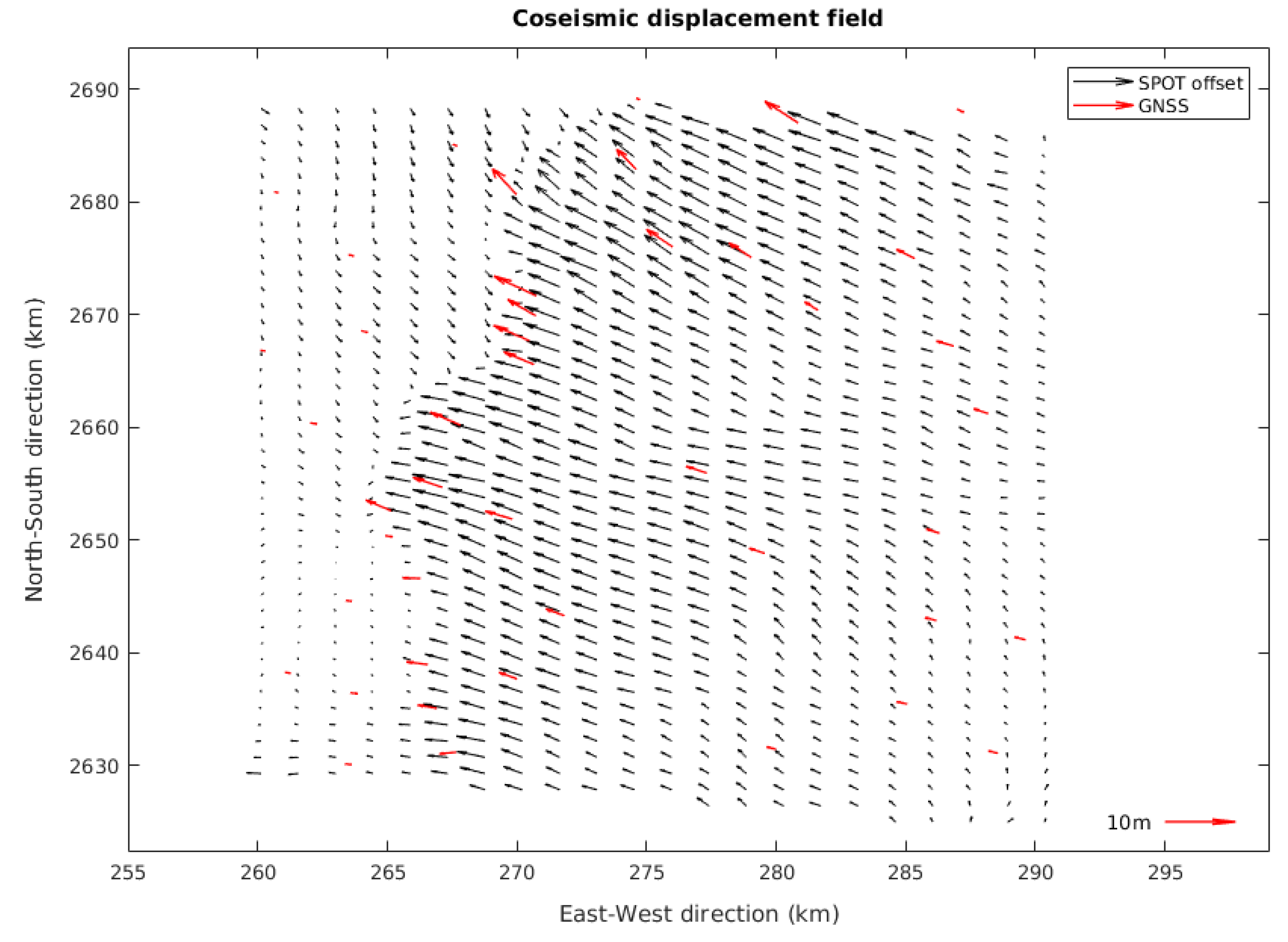
2.4. Sub-Pixel Correlation of SPOT Images

In order to obtain observations of the hanging-wall, the COSI-Corr (Co-registration of Optically Sensed Images and Correlation) software was used to correlate pre- and post-earthquake optical images. SPOT satellite panchromatic images were processed to determine the horizontal coseismic displacement using the subpixel correlation technique ([23,24]). In this study, we used SPOT 1-2 images with a 10 m resolution and with lower cloud coverage (see Table 2). The locations of the SPOT images are showed by the orange dashed box in Figure 1A. The pre-earthquake image is from 29 January 1999 and 2 months following the event for the second image (23 November 1999). In order to minimize uncertainties in the correction of topographic effects, we selected images covering the area with near-vertical incidence angle ( 2 . 9 ° for the pre-earthquake image and 2 . 5 ° for the post one). We used a Tandem-X DEM with a spatial resolution of 12.5 m for the processing as the resolution of the images is 10 m (InSAR resolution is 80 m). Even though the images selected are covering 8 months before the event and two months after, no significant pre-seismic deformation was present on the GPS observations and only a few cm of horizontal post-seismic deformation, so we considered that the offsets are essentially representing the co-seismic displacements [10].
In order to obtain the ground deformation, SPOT pairs were processed using COSI-Corr. It is a module developed in IDL (Interactive Data Language) and integrated in ENVI (Environment for Visualizing Images) by the Caltech Tectonics Observatory (USA). The methodology allows an automatic and precise orthorectification and coregistration of satellite images [25]. The main steps of the procedure are an ortho-rectification of the primary image with Tandem-X DEM due to precise selection of ground control points (GCPs), then ortho-rectification of the secondary image using GPS data values in the far field to correct for long wavelength bias. An optimization is applied to improve the ortho-rectification—reduction of the mis-registration unavoidable from the manual tie points selection by optimizing the GCPs of the secondary image (iteration until ground offset between the primary and secondary images is negligible). Finally, the subpixel correlation of the pre and post-event ortho images leads to three bands (East-West (Figure 5A) and North-South offset fields (Figure 5B)), and the Signal-to-Noise ratio from which the horizontal ground displacement is retrieved. For the joint inversion, we only kept pixels with a Signal-To-Noise ratio (SNR) above 0.1 and removed the area covered by clouds. An RMS (Root Mean Square) of about 2 m is present between GPS and SPOT offsets (Figure 6) mainly due to the different number of points and the issues in the far field. Long-wavelength artifacts are observed on the offsets (see Figure 5), mainly for the North-South image, due to satellite attitude changes.

3. Earthquake Modelling

Okada’s dislocation theory [26] has been generally used to study and invert seismic fault displacements. However, it only works under the assumption that the Earth crust is a homogeneous elastic half-space and for near-field observations, as the Earth’s curvature and radial heterogeneity are not taken into account in Okada’s equations. This standard dislocation model calculates an analytical solution for ground deformation due to shear and tensile faults. The fault is modelled by a rectangular geometry (defined by length, width, depth, strike, dip and 3-component dislocation amplitude (rake, slip and opening)) which is decomposed into small dislocation patches. This theory will be used to determine the slip distribution in this study.
From previous models available for the Chi-Chi event in the literature as presented in the introduction of this paper, inconsistencies are observed between rupture processes of the earthquake using one or multiple types of observations. For instance, inconsistencies due to the quality of the data sets: low density of GPS points and low coherence of InSAR, non-negligible residuals between observations and model or the type of dislocation model used introducing overlaps and gaps.
The proposed method in this paper combines five data types in a joint inverse model and thus requires a precise estimation of relative weighting of each data set. In that objective, the generalized Akaike’s Bayesian Information Criterion (gABIC) is used.
Furthermore, before estimating the relative weights and inverting the data, in order to make the computation feasible and efficient, InSAR observations are often down-sampled to limited numbers of points (from several thousand points to a few hundred). The Quadtree method [27] was used and displacement gradients are used to determine the sub-sampling window size. Before this, a linear trend is removed from the interferograms (to remove the orbital ramp).

3.1. Generalized Akaike’s Bayesian Information Criterion (gABIC)

A precise weighting of each data set is fundamental to realize the joint inversion. These weightings strongly affect the result of the inversion (as explained in Reference [28]). For instance, an over-weighting of one data set could induce an under-weighting of the other data sets and disturb the estimation of each parameter of the fault geometry. In that goal, the weight determination method developed by Yi ([29,30]) is used: gABIC based on the entropy maximization principle [31] to determine the regularization parameter (a spatial constraint used to regulate the rupture process), and the Bayesian theorem to estimate the probability distribution of the slip for given observations (GPS, benchmarks, levelling, InSAR, SPOT offsets) and prior constraints (Laplacian constraint in our case). In this generalized version, the type of observations and prior constraints do not need to be specified; only diagonal covariance matrices have to be estimated before running gABIC script.
As we have 8 sets of (pseudo-) observations (3 interferograms, GPS, benchmarks, levelling and SPOT offsets in addition to the Laplacian constraint), 7 hyperparameters need to be determined using the search-based gABIC method. To obtain optimal weight ratios that minimize the ABIC value, large enough ranges of these hyperparameters have to be considered. In practice, searching the seven data sets with a small enough interval is highly time consuming. In order to reduce the processing time, a first estimation of each relative weight was done by calculating it for each data set in respect with the GPS one, which covers the whole area with a low uncertainty. For this first step, the weighting range was determined using a power law method ( 10 x ) and then refined using a linear method (x) for the interval of inputs (x representing the values to test). Once the interval of hyperparameter was reduced, gABIC could be used using several data sets at once.
The inversion equations [30] are the following (to make the equations more manageable, only one interferogram is mentioned):
d = H a + e
0 = S a + ϵ ,
with:
  • d = [ d G P S d B e n c h d l e v d I n S A R d S P O T ] N x 1 T : Nx1 vector containing 5 data types (total N observations);
  • H = [ H G P S H B e n c h H l e v H I n S A R H S P O T ] N x M T : NxM coefficient matrix;
  • S = [ S S ] P x M T : P x M coefficient matrix containing Prior constraints
  • a is a M dimensional model parameter vector that varies with the time windows;
  • e = [ e G P S e B e n c h e l e v e I n S A R e S P O T ] N x 1 T & ϵ = [ ϵ S ] P x 1 T : are vectors of the Gaussian-distributed uncertainties of observations and constraints, respectively.
Furthermore, e Q ˜ ( σ i 2 ) where Q ˜ ( σ i 2 ) = σ G P S 2 with Q (i refers to the five data sets) covariance matrices of observations and a similar equation for the constraint). The covariance matrix Q is expressed as follows (blkdiag means block diagonal matrix):
Q = b l k d i a g Q ˜ G P S σ B e n c h 2 σ G P S 2 . Q ˜ B e n c h σ l e v 2 σ G P S 2 . Q ˜ l e v σ I n S A R 2 σ G P S 2 . Q ˜ I n S A R σ S P O T 2 σ G P S 2 . Q ˜ S P O T N x N
The ABIC function was first introduced by Reference [32], using only static GPS observations and Laplacian spatial constraint, as:
A B I C = N · l o g s ( a * ) M · l o g α 2 + l o g | | H T E 1 H + α 2 G | | + l o g | | E | | l o g | | S T S | | + N ( l o g ( 2 π ) l o g N + 1 ) .
gABIC is the generalized version, it searches for the hyperparameters ( σ i 2 ) that minimize the ABIC value as presented in Reference [29]:
A B I C = N · l o g s ( a * ) M · l o g α 2 + l o g | | H T E ( σ i 2 ) 1 H + α 2 ( S T S ) Δ ( ϵ i 2 ) 1 | | + l o g | | E ( σ i 2 ) | | l o g | | ( S T S ) Δ ( ϵ i 2 ) 1 | | + N ( l o g ( 2 π ) l o g N + 1 ) ,
where:
  • α 2 = σ G P S 2 ϵ S 2 is the smoothness parameter;
  • ϵ i is a hyperparameter representing the weight of the constraint;
  • s ( a ) = ( d H a ) T Q 1 ( d H a ) + α 2 a T ( S T S ) Δ 1 a .

3.2. Modelling Strategy: Fault Geometry and Slip Distribution

Regarding the fault geometry (Table 3), this study was based on the previous model designed by References [14,17] and adjusted in accordance with the more recent literature as described in the introduction. Reference [14] is in agreement with the geologically constrained fault model of Reference [33]. Mainly the decollement subfault was adjusted: especially the depth and dip and the rakes of each sub-fault according to the inversion of our data sets. The decollement was fixed arbitrarily to be wide enough so that insignificant slip occurred at one edge of it. Furthermore, for segments 2 and 3, we tried to avoid as many gaps and overlaps as possible. The purpose of the study was to test gABIC on a complicated but known case including several data sets, not to determine the most precise fault geometry. However, for more precision and physical reality a triangular dislocation model would be necessary. Poly3d will be used in a future work [34].
Under the assumption of an elastic homogeneous half-space, the fault geometry and the slip distribution are determined following a 2-step approach using the Particle Swarm Optimization and OKada INVersion package (PSOKINV). It is a geodetic inversion package [35] developed in Matlab which can solve linear and nonlinear problems. Multiple geodetic data sets can be handled by the program.
First, a nonlinear inversion is performed to determine the fault parameters (location, strike, dip, rake, length, width, depth and slip) minimizing the square misfit under the hypothesis of a uniform slip on a rectangular fault using the multi-peak particle swarm optimization (M-PSO) [36], a non linear algorithm approach based on the elastic Okada dislocation models [26]. The slip distribution is then determined as a linear problem, and optimally-smoothed parameters are obtained. This is an iterative technique for estimating optimal dip angle and smoothing factors based on a conjugate gradient least square method. When all the parameters are optimally determined, the fault plane was discretized into rectangular sub-patches of 2 km × 2 km (see Figure 7).

4. Data Set Weighting

4.1. Benefit of Multiple Data Sets

The Chi-Chi earthquake is a particularly interesting event to work on a joint inversion methodology as it has been well studied already, its fault geometry is quite stabilised and the island is well monitored so a large variety of data sets is available from satellite images (ERS and SPOT) to field measurements (levelling, benchmarks, GPS in our case).
As explained previously, geodetic observations were selected with their advantages and disadvantages but presenting a good temporal and spatial complementarity. Figure 8 presents the slip distribution obtained for each data set alone to see its impact to the overall slip distribution. For the GPS based slip distribution (Figure 8A) and adding benchmark and levelling data (Figure 8B), similar patterns as the one presented in Reference [14] are observed. The maximum of the slip occurs near the surface at the northwestern edge of the fault and negligible slip is present below 10 km depth. The contribution of benchmark and levelling data sets in addition to GPS is useful to get more information in the curved part (where the slip has the highest magnitude and where the geometry of the fault may not be optimal). A shallower slip distribution is visible in comparison to GPS alone (especially subfaults 2 and 3) and we obtain more precision about the vertical movement. From InSAR observations (the result from the interferogram 28 October 1999–15 July 1999 is presented in Figure 8C), the slip is under-estimated in comparison with GPS data due to its asymmetrical distribution, only covering the footwall. This is also why we do not observe any signal on the decollement at depth. Finally, Figure 8D, from only SPOT offsets, is not over- or under-estimating the slip but showing more deformation at depth mainly due to the large uncertainties in the far-field.

4.2. gABIC Impact

It is essential in the joint inversion to determine the relative weights between the different data sets and the constraint to properly balance the contributions of each of them. The difference with previous studies is the use of the generalized formula of the ABIC method ([31]) from Reference [29] (gABIC) to be able to take into account any type of data sets without need of specification and different type of constraints. The point of using gABIC is to obtain a precise value for the weight of each data set that is used for the estimation of the slip distribution. The main issue with this method is that it is computationally intensive. In order to reduce the processing time, the following strategy was followed. First each data set was run separately with the GPS as reference to estimate the relative weight of this data set in relation to the GPS. Then, when a first estimation was made, we could run all data sets together by restricting the search intervals.
The first row of Figure 9 presents the slip distribution obtained from GPS and the three interferograms where first all the weights were set to 1 and secondly the weights were estimated by gABIC. The second row is presenting the slip distribution obtained from all the data sets used jointly following the same steps: first the weights were set to 1, then weights were estimated by gABIC.
After the estimation of the relative weights by gABIC, we can see that the slip distributions are smoother, with a maximum of slip at the curve of the fault of about 12 m. No unexpected slip is present on the edge of the fault. The weights for the benchmarks and levelling is low because the spatial extent of the data sets is small in comparison with the other data sets even though their precision is better.

5. Seismic Hazard

The seismic moment was estimated based on the inverted slip distribution, with a maximum at 3.9 × 10 20 N · m:
M 0 = μ · S · δ u
μ : Shear modulus taken as 33 GPa,
S: Area of the fault,
δ u: Mean slip from strike slip and dip slip.
The seismic moment release was summed for each 2 × 2 km patch in horizontal rows to obtain the variation in moment release with depth, and summed in vertical columns to get the moment release along strike. The slip distribution and the study of the integrated moment by depth and strike show that the main deformation happened in the north part of the fault, where the fault is curving towards the east with a slip reaching 12.6 m (Figure 9D) and most of the moment was released at depths shallower than 4 km.
To evaluate the effect of the rupture on the surrounding area, the Coulomb Stress Change (CSC) was calculated using Coulomb 3.3 (Graphic-Rich Deformation and Stress-Change Software) USGS software [37,38]. CSC represents the transfer of stress. It is possible to estimate, from the CSC, the triggering effect of large earthquakes such as the Chi-Chi event. CSC was estimated on a specified fault (strike, dip, and rake specified) at a depth of 11 km with a friction coefficient of 0.4. Figure 10 shows that the increase of Coulomb stress is concentrated at the north of the Chelungpu fault and towards the north-east which indicates that most of the stress was transfered to faults at the north of the Chelungpu fault. As presented by Reference [16], aftershocks (see Figure 11) mainly occured downdip from the rupture area which is consistent with the increase of Coulomb stress that we observe in Figure 10A. We observe in Figure 10B an increase of stress for depth above 10 km which is consistent with the aftershock distribution.

6. Conclusions

The Chi-Chi earthquake is a complicated event that was caused by the reactivation of the Chelungpu fault whose geometry is quite complex and which occurs in a region of steep topography and dense vegetation.
Five types of geodetic observations (GPS, levelling, benchmarks, InSAR and SPOT offsets) were combined to determine the fault slip distribution of the 1999 Chi-Chi earthquake. A methodology was established in order to precisely estimate the relative weights between the data sets, which is a critical step for the modelling. A wrong estimation will create an under or over-estimation of the slip distribution. For this purpose, the generalized ABIC formula was applied to estimate the relative weights between the observations and the constraint. The slip distribution is mainly determined by the GPS as presented in previous papers, however the incorporation of other geodetic observations constrains the model especially on the curved part of the fault.
The preferred slip distribution including all the data sets and using the relative weights estimated by gABIC shows that the maximum slip was 12.6 m on the north curved part of the fault with a seismic moment of 3.9 × 10 20 N · m, corresponding to a magnitude of M w 7.6. The study of the moment and Coulomb Stress Changes show that most of the slip happened on the north part of the fault at shallow depths and that most the energy released by the event was transferred to the faults at the north of the area, which is now the most probable location of a future event.
In the last decade, satellite images have dramatically improved especially with the Sentinel constellation and the evolution of atmospheric methods, as well as the densification of GPS networks. It is essential to take advantage of all these data, to take into account their quality and coverage by estimating precise relative weights and thus to establish methodology to precisely monitor the earth deformation.

Author Contributions

M.R. did the processing, performed the result analysis and wrote the manuscript. Z.L. and P.C. provided suggestions on the processing and analysis and reviewed the manuscript. C.S., W.F. and L.Y. provided information for gABIC and PSOKINV. J.-C.H. provided data resources. All authors have read and agreed to the published version of the manuscript.

Funding

This research was funded by ESA-MOST DRAGON-4 project, grant number 32244. Part of the work was also supported by the UK NERC through the Centre for the Observation and Modelling of Earthquakes, Volcanoes and Tectonics (COMET, Ref.: come30001) and the LICS project (Ref. NE/K010794/1).

Acknowledgments

Some figures were made using the Generic Mapping Tools by Reference [39]. ERS data were provided by ESA and SPOT images by Airbus Defence and Space.

Conflicts of Interest

The authors declare no conflict of interest.

Abbreviations

The following abbreviations are used in this manuscript:
CGSCentral Geological Survey
COSI-CorrCo-registration of Optically Sensed Images and Correlation
CSCCoulomb Stress Change
CWBCentral Weather Bureau
DEMDigital Elevation Model
ENVIEnvironment for Visualizing Images
ERSEuropean Remote-Sensing Satellite
ESAEuropean Space Agency
gABICGeneralized Akaike’s Bayesian Information Criterion
GCPGround Control Point
GPSGlobal Positioning System
IDLInteractive Data Language
IESASInstitute of Earth Sciences, Academia Sinica
InSARInterferometric Synthetic Aperture Radar
MOEAMinistry of Economic Affairs
MOIMinistry of Interior
M-PSOMulti-peak Particle Swarm Optimization
PSOKINVParticle Swarm Optimization and Okada Inversion package
RMSRoot Mean Square
SNAPSentinel Application Platform
SNAPHUStatistical-cost, Network-flow Algorithm for Phase Unwrapping
SNRSignal-To-Noise Ratio
SPOTSatellite Pour l’Observation de la Terre
SRTMShuttle Radar Topography Mission
TWD67Transverse Mercator Two-degree Grid 1967
USGSUnited States Geological Survey
WGS84World Geodetic System 1984

References

  1. Ching, K.E.; Hsieh, M.L.; Johnson, K.; Chen, K.; Rau, R.J.; Yang, M. Modern vertical deformation rates and mountain building in Taiwan from precise leveling and continuous GPS observations, 2000–2008. J. Geophys. Res. 2011, 116. [Google Scholar] [CrossRef]
  2. Ma, K.F.; Mori, J.; Lee, S.J.; Yu, S.B. Spatial and Temporal Distribution of Slip for the 1999 Chi-Chi, Taiwan, Earthquake. Bull. Seismol. Soc. Am. 2001, 91, 1069–1087. [Google Scholar]
  3. Wang, J.H. Studies of Earthquake Energies in Taiwan: A Review. Terr. Atmos. Ocean. Sci. 2016, 27, 1–19. [Google Scholar] [CrossRef]
  4. Lee, Y.H.; Shih, Y.X. Coseismic displacement, bilateral rupture, and structural characteristics at the southern end of the 1999 Chi-Chi earthquake rupture, central Taiwan. J. Geophys. Res. 2011, 116. [Google Scholar] [CrossRef]
  5. Lee, J.C.; Chen, Y.G.; Sieh, K.; Mueller, K.; Chen, W.S.; Chu, H.T.; Chan, Y.C.; Rubin, C.; Yeats, R. A Vertical Exposure of the 1999 Surface Rupture of the Chelungpu Fault at Wufeng, Western Taiwan: Structural and Paleoseismic Implications for an Active Thrust Fault. Bull. Seismol. Soc. Am. 2001, 91, 914–929. [Google Scholar] [CrossRef]
  6. Pathier, E.; Fruneau, B.; Deffontaines, B.; Angelier, J.; Chang, C.; Yu, S.; Lee, C. Coseismic displacements of the footwall of the Chelungpu fault caused by the 1999, Taiwan, Chi-Chi earthquake from InSAR and GPS data. Earth Planet. Sci. Lett. 2003, 212, 73–88. [Google Scholar] [CrossRef]
  7. Lee, J.C.; Chan, Y.C. Structure of the 1999 Chi-Chi earthquake rupture and interaction of thrust faults in the active fold belt of western Taiwan. J. Asian Earth Sci. 2007, 31, 226–239. [Google Scholar] [CrossRef]
  8. Angelier, J.; Lee, J.C.; Chu, H.T.; Hu, J.C.; Lu, C.Y.; Chan, Y.C.; Tin-Jai, L.; Font, Y.; Deffontaines, B.; Yi-Ben, T. Le séisme de Chi-Chi (1999) et sa place dans l’orogène de Taiwan. Comptes Rendus de l’Academie de Sciences Serie IIa: Sciences de la Terre et des Planetes 2001, 333, 5–21. [Google Scholar] [CrossRef]
  9. Yu, S.B.; Kuo, L.C.; Hsu, Y.J.; Su, H.H.; Liu, C.C.; Hou, C.S.; Lee, J.F.; Lai, T.C.; Liu, C.C.; Liu, C.L.; et al. Preseismic Deformation and Coseismic Displacements Associated with the 1999 Chi-Chi, Taiwan, Earthquake. Bull. Seismol. Soc. Am. 2001, 91, 995–1012. [Google Scholar] [CrossRef]
  10. Dominguez, S.; Avouac, J.P.; Michel, R. Horizontal coseismic deformation of the 1999 Chi-Chi earthquake measured from SPOT satellite images: Implications for the seismic cycle along the western foothills of central Taiwan. J. Geophys. Res. 2003, 108. [Google Scholar] [CrossRef] [Green Version]
  11. Kuo, Y.; Ayoub, F.; Leprince, S.; Chen, Y.; Avouac, J.; Shyu, J.; Lai, K.; Kuo, Y. Coseismic thrusting and folding in the 1999 Mw 7.6 Chi-Chi earthquake: A high-resolution approach by aerial photos taken from Tsaotun, central Taiwan. J. Geophys. Res. Solid Earth 2014, 119, 645–660. [Google Scholar] [CrossRef] [Green Version]
  12. Loevenbruck, A.; Cattin, R.; Le Pichon, X.; Courty, M.; Yu, S. Seismic cycle in Taiwan derived from GPS measurements. Comptes rendus de l’Académie des Sciences serie II Fascicule A-Sciences de la terre et des planètes 2001, 333, 57–64. [Google Scholar] [CrossRef]
  13. Okada, Y. Internal deformation due to shear and tensile faults in a half-space. Bull. Seismol. Soc. Am. 1992, 82, 1018–1040. [Google Scholar]
  14. Johnson, K.; Segall, P. Imaging the ramp–decollement geometry of the Chelungpu fault using coseismic GPS displacements from the 1999 Chi-Chi, Taiwan earthquake. Tectonophysics 2004, 378, 123–139. [Google Scholar]
  15. Zhang, L.; Wu, J.C.; Ge, L.L.; Ding, X.L.; Chen, Y.L. Determining fault slip distribution of the Chi-Chi Taiwan earthquake with GPS and InSAR data using triangular dislocation elements. J. Geodyn. 2008, 45, 163–168. [Google Scholar] [CrossRef]
  16. Hsu, Y.J.; Avouac, J.P.; Yu, S.B.; Chang, C.H.; Wu, Y.M.; Woessner, J. Spatio-temporal Slip, and Stress Level on the Faults within the Western Foothills of Taiwan: Implications for Fault Frictional Properties. Pure Appl. Geophys. 2009, 166, 1853–1884. [Google Scholar] [CrossRef] [Green Version]
  17. Johnson, K.M.; Hsu, Y.J.; Segall, P.; Yu, S.B. Fault geometry and slip distribution of the 1999 Chi-Chi Taiwan earthquake imaged from inversion of GPS data. Geophys. Res. Lett. 2001, 28, 2285–2288. [Google Scholar] [CrossRef] [Green Version]
  18. Huang, C.; Chan, Y.C.; Hu, J.C.; Angelier, J.; Lee, J.C. Detailed surface co-seismic displacement of the 1999 Chi-Chi earthquake in western Taiwan and implication of fault geometry in the shallow subsurface. J. Struct. Geol. 2008, 30, 1167–1176. [Google Scholar] [CrossRef]
  19. Chen, C.W.; Zebker, H.A. Network approaches to two-dimensional phase unwrapping: Intractability and two new algorithms. J. Opt. Soc. Am. 2000, 17, 401–414. [Google Scholar] [CrossRef]
  20. Chen, C.W.; Zebker, H.A. Two-dimensional phase unwrapping with use of statistical models for cost functions in nonlinear optimization. J. Opt. Soc. Am. 2001, 18, 338–351. [Google Scholar] [CrossRef] [PubMed] [Green Version]
  21. Chen, C.W.; Zebker, H.A. Phase unwrapping for large SAR interferograms: Statistical segmentation and generalized network models. IEEE Trans. Geosci. Remote. Sens. 2002, 40, 1709–1719. [Google Scholar] [CrossRef] [Green Version]
  22. Goldstein, R.; Werner, C. Radar interferogram filtering for geophysical applications. Geophys. Res. Lett. 1998, 25, 4035–4038. [Google Scholar] [CrossRef] [Green Version]
  23. Van Puymbroeck, N.; Michel, R.; Binet, R.; Avouac, J.; Taboury, J. Measuring earthquakes from optical satellite images. Appl. Opt. 2000, 39, 3486–3494. [Google Scholar] [CrossRef] [PubMed]
  24. Michel, R.; Avouac, J.; Taboury, J. Measuring near field coseismic displacements from SAR images: Application to the Landers earthquake. Geophys. Res. Lett. 1999, 26, 3017–3020. [Google Scholar] [CrossRef] [Green Version]
  25. Leprince, S.; Barbot, S.; Ayoub, F.; Avouac, J. Automatic and Precise Ortho-rectification, Coregistration, and Subpixel Correlation of Satellite Images, Application to Ground Deformation Measurements. IEEE Trans. Goesci. Rmote Sens. 2007, 45, 1529–1558. [Google Scholar] [CrossRef] [Green Version]
  26. Okada, Y. Surface deformation due to shear and tensile faults in a half-space. Bull. Seismol. Soc. Am. 1985, 75, 1135–1154. [Google Scholar]
  27. Jonsson, S.; Zebker, H.; Segall, P.; Amelung, F. Fault Slip Distribution of the 1999 Mw 7.1 Hector Mine, California, Earthquake, Estimated from Satellite Radar and GPS Measurements. Bull. Seismol. Soc. Am. 2002, 92, 1377–1389. [Google Scholar] [CrossRef]
  28. Funning, G.; Fukahata, Y.; Yagi, Y.; Parsons, B. A method for the joint inversion of geodetic and seismic waveform data using ABIC: Application to the 1997 Manyi, Tibet, earthquake. Geophys. J. Int. 2014, 196, 1564–1579. [Google Scholar] [CrossRef] [Green Version]
  29. Yi, L.; Xu, C.; Zhang, X.; Wen, Y.; Jiang, G.; Li, M.; Wang, Y. Joint inversion of GPS, InSAR and teleseismic data sets for the rupture process of the 2015 Gorkha, Nepal, earthquake using a generalized ABIC method. J. Asian Earth Sci. 2017, 148, 121–130. [Google Scholar] [CrossRef]
  30. Yi, L.; Xu, C.; Wen, Y.; Zhang, X.; Jiang, G. Rupture process of the 2016 Mw 7.8 Ecuador earthquake from joint inversion of InSAR data and teleseismic P waveforms. Tectonophysics 2018, 722, 163–174. [Google Scholar] [CrossRef]
  31. Akaike, H. Information theory and an extension of the maximum likelihood principle. In Selected Papers of Hirotugu Akaike; Springer: New York, NY, USA, 1973; pp. 267–281. [Google Scholar]
  32. Yabuki, T.; Matu’ura, M. Geodetic data inversion using a Bayesian information criterion for spatial distribution of fault slip. Geophys. J. Int. 1992, 109, 363–375. [Google Scholar] [CrossRef]
  33. Yue, L.F.; Suppe, J.; Hung, J.H. Structural geology of a classic thrust belt earthquake: The 1999 Chi-Chi earthquake Taiwan (Mw = 7.6). J. Struct. Geol. 2005, 27, 2058–2083. [Google Scholar] [CrossRef]
  34. Maerten, F.; Maerten, L.; Pollard, D. iBem3D, a three-dimensional iterative boundary element method using angular dislocations for modeling geologic structures. Comput. Geosci. 2014, 72, 1–17. [Google Scholar] [CrossRef]
  35. Feng, W.; Li, Z.; Elliott, J.; Fukushima, Y.; Hoey, T.; Singleton, A.; Cook, R.; Xu, Z. The 2011 Mw 6.8 Burma earthquake: Fault constraints provided by multiple SAR techniques. Geophys. J. Int. 2013, 195, 650–660. [Google Scholar] [CrossRef] [Green Version]
  36. Feng, W.; Li, Z. A novel hybrid PSO/simplex algorithm for determining earthquake source parameters using InSAR observations. Diqiu Wulixue Jinzhan Progress Geophys. 2010, 25, 1550–1559. [Google Scholar] [CrossRef]
  37. Toda, S.; Stein, R.S.; Richards-Dinger, K.; Bozkurt, S. Forecasting the evolution of seismicity in southern California: Animations built on earthquake stress transfer. J. Geophys. Res. 2005, 110. [Google Scholar] [CrossRef]
  38. Lin, J.; Stein, R. Stress triggering in thrust and subduction earthquakes, and stress interaction between the southern San Andreas and nearby thrust and strike-slip faults. J. Geophys. Res. 2004, 109. [Google Scholar] [CrossRef] [Green Version]
  39. Wessel, P.; Smith, W. New, improved version of Generic Mapping Tools released. EOS Trans. Am. Geophys. Union 1998, 79, 579. [Google Scholar] [CrossRef]
Figure 1. (A) Geodynamic map of Taiwan. The Chelungpu thrust fault is shown in red (National Taiwan University) and the other faults in yellow (National Taiwan University). Focal mechanism of the Chi-Chi earthquake on the inset map (USGS: 23.772 ° N 120.982 ° E). Seismicity (from 1998 to 2000, source National Taiwan University) over Taiwan. GPS displacement vectors ([9]) shown by black arrows. Green dashed box shows the location of the ERS-2 scenes from descending track 232, orange dashed box shows the location of the SPOT satellite images used in this study. The purple dashed box is the location of the benchmark data, results are presented in (B) for the footwall displacements and in (C) for the hanging-wall displacements (notice the different scale). Finally, the blue dashed box is the location of the levelling data, results are presented in (D).
Remotesensing 12 03125 g001
Figure 2. (A) Levelling and (B) geodetic benchmark in Taichung city, Taiwan and (C) a GPS antenna in Puli City, Taiwan. [Photo credit: Marine Roger].
Remotesensing 12 03125 g002
Figure 3. Levelling deformation profiles of 2 lines: (A) WU007-AF27, (B) T001-T045. See Figure 1D for profile locations.
Remotesensing 12 03125 g003
Figure 4. Interferograms of the Chi-Chi earthquake (color bar in cm) as presented in Table 1, the primary image is on 28 October 1999. (A) 28/10/1999-21/01/1999. (B) 28/10/1999-06/05/1999. (C) 28/10/1999-15/07/1999.
Remotesensing 12 03125 g004
Figure 5. (A,B) East-West and North-South horizontal offsets obtained from the sub-pixel correlation of the two SPOT images (see Table 2) acquired before and after the earthquake (scale in m). Grey areas are where the correlation was too low. (Mean and standard deviation for EW band: −1.5 m, 1.7 m and for NS band: 1.2 m, 1.9 m).
Remotesensing 12 03125 g005
Figure 6. Coseismic displacement vectors, black arrows represent SPOT offsets and red arrows GPS data.
Remotesensing 12 03125 g006
Figure 7. Fault geometry used in this study (Table 3).
Remotesensing 12 03125 g007
Figure 8. Slip distribution model for 4 sub-faults geometry for the Chelungpu fault (scale bars in m). Inversion (Correlation coefficient, RMS (m)) based on (A) GPS only (0.96, 0.39); (B) GPS, benchmarks and levelling (0.57, 3); (C) One interferogram (15 July 1999) (0.90, 0.03); (D) SPOT offset only (0.91, 0.90). The colour scale saturates at 12 m. M 0 is the total seismic moment for each model.
Remotesensing 12 03125 g008
Figure 9. Slip distribution model. Inversion based on (A) GPS data and three interferograms (Table 1) with all the weights set to 1; (B) same data sets but with the relative weights estimated by gABIC (GPS 1, 0.09, 0.10, 0.10 for the three interferograms). All the data sets were included in (C,D). (C) The relative weights are set to 1; (D) the relative weights ([GPS, levelling, Benchmarks, Interferogram 1, 2, 3, SPOT] = [1, 10 4 , 10 4 , 0.09, 0.10, 0.10, 0.01]) were estimated by gABIC. The colour scale saturates at 12 m. M 0 is the total seismic moment for each model.
Remotesensing 12 03125 g009
Figure 10. (A) Coulomb Stress Changes (CSCs) due to the Chi-Chi earthquake. The green lines are the location of the 4 sub-faults. (B) Cross section with location presented on (A) by the dashed line.
Remotesensing 12 03125 g010
Figure 11. (A) Position of the chelungpu fault (in red) and the fault geometry in black. Dots are representing the aftershocks during the 6 months following the event. Larger dots: M w 5 , small ones 3 M w < 5 . (B) A-B profile showing the aftershocks in depth (m).
Remotesensing 12 03125 g011
Table 1. ERS-2 data used in this study.
Acquisition DateTrackFrameOrbitTemporal Baseline [Days]Perp. Baseline [m]Height Ambiguity [m]
28 October 1999232312323633---
21 January 1999232312319625280.00−92.89102.07
06 May 1999232312321128175.0020.08−469.46
15 July 1999232312322130105.00−247.7138.28
Table 2. SPOT data used in this study, resolution 10 m.
Acquisition DateSatellite/Orient.Cloud CoverIncidence AngleOrient. AngleSun ElevationSun Azimuth
29 January 1999SPOT2/Right 10 % 2.9° 9.4° 42.9° 151.0°
23 November 1999SPOT1/Right 0 % 2.5° 9.4° 43.4° 159.7°
Table 3. Fault geometry parameters used in this study and the ones from Reference [14]. [SRCMOD: Earthquake Source Model Database (http://equake-rc.info/srcmod/)].
This StudyLengthWidthDepthDipStrikeRake
Segment 171.45 km30 km0 km 23 ° 3.3° 62°
Segment 210 km10 km0 km22° 50° 90°
Segment 315 km20 km0 km24° 88° 90°
Segment 470 km34 km11.7 km5.7° 3.3° 54°
[14,17]
(SRCMOD)
Segment 170 km30 km0 km23° [22–31]3.3° ?
Segment 28.6 km30 km0 km23° [13–30]35° ?
Segment 327 km [22–35]30 km0 km21° [14–41]88° [49–94]?
Segment 470 km?[5.8–8.6] km[0–7]° 88° ?

