Abstract
Automatic ship detection in optical remote sensing images is of great significance due to its broad applications in maritime security and fishery control. Most ship detection algorithms utilize a single-band image to design low-level and hand-crafted features, which are easily influenced by interference like clouds and strong waves and not robust for large-scale variation of ships. In this paper, we propose a novel coarse-to-fine ship detection method based on discrete wavelet transform (DWT) and a deep residual dense network (DRDN) to address these problems. First, multi-spectral images are adopted for sea-land segmentation, and an enhanced DWT is employed to quickly extract ship candidate regions with missing alarms as low as possible. Second, panchromatic images with clear spatial details are used for ship classification. Specifically, we propose the local residual dense block (LRDB) to fully extract semantic feature via local residual connection and densely connected convolutional layers. DRDN mainly consists of four LRDBs and is designed to further remove false alarms. Furthermore, we exploit the multiclass classification strategy, which can overcome the large intra-class difference of targets and identify ships of different sizes. Extensive experiments demonstrate that the proposed method has high robustness in complex image backgrounds and achieves higher detection accuracy than other state-of-the-art methods.
1. Introduction
Automatic ship detection has attracted great research interest due to its broad applications in both the military and civil domain, such as national defense construction, maritime security, port surveillance, and sea traffic control [1]. Many previous studies on ship detection were mainly based on synthetic aperture radar (SAR) images [2,3,4,5,6,7,8,9,10,11,12], because they are less impacted by adverse weather conditions. Recently, it became a wide trend for satellites to be equipped with multiple sensors collecting multi-resolution optical remote sensing images from multispectral and panchromatic bands [13], such as QuickBird, SPOT-5, GaoFen-1, GaoFen-2, Venezuelan Remote Sensing Satellites (VRSSs), and so on. Some researchers [14,15,16,17] have paid more attention to detecting ships with optical remote sensing images since they generally have higher resolutions and share clearer spatial details than SAR images.
Nevertheless, ship detection performance in optical remote sensing images usually suffers from three main problems: (1) a large data volume of optical remote sensing imagery [15,18,19], (2) the interference of complex factors such as clouds and strong waves [15,16,19,20], and (3) the large-scale variation of ships (from dozens of pixels to thousands) [16,20]. In the past few years, many ship detection algorithms [21,22,23,24,25] have been proposed. Most of them take a hierarchical method whose algorithm flow can be roughly divided into three stages: sea-land segmentation, ship candidate region extraction, and ship classification. The first stage, sea-land segmentation, aims to remove the land regions and preserve the sea area by utilizing some simple and fast methods, like a priori geographic information [14,15] or Otsu threshold segmentation [19]. The complex land surface usually leads to many false alarms during the detection process. Therefore, it is necessary to mitigate the effects of land regions by sea-land segmentation. The second stage, ship candidate region extraction, aims to extract potential candidate regions of ship targets from remote sensing images. Some typical methods in this stage include sliding window [22,26], saliency-based methods [16,27,28,29], and wavelet-transformation-based methods [17,19]. At the last ship classification stage, each candidate region will be usually identified as a ship target or a non-ship target by feature representation and binary classification. Earlier related works on this stage mainly used specially designed hand-crafted features to detect ships, including shape [21], texture [14,26], ship histogram of oriented gradient (S-HOG) [16,22], gist [27], structure local binary pattern (structure-LBP) [30], and different combinations of these features [14,17,29]. With these features, a classifier will be used to distinguish ships from false alarms, such as AdaBoost [31], support vector machine (SVM) [14,15], and extreme learning machine (ELM) [19].
Previous research has established some basic ship detection frameworks. Gan et al. [22] proposed the continuous interval rotating detection sliding window of the HOG (histogram of oriented gradients) feature to detect potential ship targets. To quickly extract ship candidate regions, Qi et al. [16] presented an unsupervised ship detection method by the visual saliency mechanism to extract candidate regions and extract S-HOG features to discriminate real ships. Nie et al. [17] proposed an effective algorithm in which morphological, geometric, and texture features of candidate regions are extracted for target confirmation. These hand-crafted features have achieved promising results, but they may lack generalization in complex weather conditions [24]. Generally speaking, the detection results of the aforementioned works are unsatisfactory with respect to complex backgrounds [20], which mainly include sea under clouds coverage, sea with strong waves, dynamic ships, and the interference of land.
With the rise of convolutional neural networks (CNNs) [32,33,34], more and more efficient object detection algorithms [35,36,37,38] have been proposed. They can be grouped into two genres on the basis of whether they generate region proposals or not, namely two stage detection methods and one stage detection methods. Region-based CNN (R-CNN) [39] is a representative example of two stage methods to adopt CNN to generate rich features for object detection, which extracts region proposals by using a selective search method. Then, a set of SVMs is used to classify each region proposal, and a linear regressor is used to refine the bounding boxes [40]. Although R-CNN outperforms previous object detection methods, the repeated computation of abundant region proposals leads to its low efficiency. SPPNet [41] and Fast R-CNN [42] are proposed to remedy this problem and obtain better detection efficiency. Faster R-CNN [37] is a further improvement of Fast R-CNN. It is the first end-to-end deep learning detector, which introduces the region proposal network (RPN) to generate nearly cost-free region proposals. In addition, the feature pyramid network (FPN) [38] extends the work of Faster R-CNN for better performance. One stage detection methods originated from you only look once (YOLO) [43], then successively from the single shot multi-box detector (SSD) [35], YOLOv2 [36], RetinaNet [44], and so on. These methods simplify detection as a regression problem. YOLO [43] adopts a single CNN backbone to directly predict class probabilities and bounding boxes from the entire image. SSD [35] introduces default boxes and multi-scale feature maps for detection, which achieves significant improvement. RetinaNet [44] proposes a new focal loss, so that the detector will put more focus on hard, misclassified examples during training.
Some remote sensing researchers have also exploited high-level semantic features to alleviate the influence of complex interferences in satellite images [45]. Tang et al. [19] extracted fast ship candidate regions in the JPEG2000 compression domain using wavelet coefficients and exploited a deep neural network (DNN) to better distinguish ship from surrounding pseudo targets. Zou et al. [15] adopted three convolutional layers and three mapping layers called SVD networks (SVDNet) to extract the features, which were fed into the SVM to verify all ship candidates and filter the false alarms. Zhang et al. [28] introduced a ship detection method based on convolutional neural networks, called S-CNN, fed with specifically designed proposals extracted from the ship model. Yang et al. [24] proposed an end-to-end framework called the rotation dense feature pyramid network (R-DFPN) that attempted to combine the dense feature pyramid network, rotation anchors, and the multiscale region of interest (ROI) alignment for ship detection. Wu et al. [20] also used the feature pyramid network (FPN) to achieve small ship detection. They proposed a coarse-to-fine detection strategy to improve the classification ability of the network. These deep learning-based methods have shown desirable performance in response to the interference of clouds and waves; however, they might produce more false alarms on land and miss small ships [18,20], thus resulting in restrictions on further improvement of ship detection performance.
Upon comprehensive consideration of the above factors, we propose a novel coarse-to-fine detection framework based on discrete wavelet transform (DWT) and a deep residual dense network (DRDN) to address these three aforementioned problems. As for the first problem about the large data volume, multispectral images of low resolution are utilized to quickly extract ship candidate regions and improve time efficiency. As for the second (the interference of clouds and waves) and third ones (large-scale variation of ships), we adopt a multiclass classification strategy to overcome the large intra-class difference of targets and identify ships of different sizes. Furthermore, DRDN is proposed to fully exploit the hierarchically semantic features from all convolutional layers and improve the classification performance on small ships.
The main contributions of this paper are as follows:
(1) A novel coarse-to-fine framework is developed for fast and accurate ship detection, which can be considered as a cascade elimination process of false alarms. Our multi-stage design aims to alleviate the above three problems. With respect to the false alarms on land, we utilize an efficient sea-land segmentation algorithm, which takes full advantage of multispectral images to achieve fast separation of land and sea.
(2) Regarding the influence of some complex interferences, we propose an enhanced DWT to highlight salient signals of ship targets and suppress interferences like waves and clouds.
(3) To improve the detection accuracy of small objects, we design the local residual dense block (LRDB) to fully extract semantic features via local residual connection and densely connected convolutional layers. Our DRDN is composed of four LRDBs to enhance dense feature fusion and boost the classification ability of the network.
(4) To further alleviate the problem of the variable sizes of ship targets and the interference of many kinds of non-ship targets, we adopt the multiclass classification strategy rather than general binary classification. The ship targets are divided into five subclasses according to their sizes and moving states. The same strategy is applied to the non-ship targets, which are also divided into five subclasses. This classification strategy aims to overcome large intra-class differences both in ship and non-ship targets; thus, a higher recall rate and a lower false alarm rate are achieved.
The remainder of this paper is organized as follows. Section 2 describes the whole framework and the details of the proposed method, including sea-land segmentation with multispectral images, ship candidate region extraction, and ship classification with DRDN. Section 3 shows the dataset setup and implementation details. The parameter setting and some comparative experiments are shown in Section 4. In Section 5, we compare our method with the state-of-the-art detectors on a remote sensing dataset, and the corresponding discussions are displayed. Finally, Section 6 concludes this paper.
2. Proposed Method
2.1. The Overall Framework
In this section, we give a detailed description of our coarse-to-fine detection framework. Figure 1 shows the workflow of the proposed method. Different from some hierarchical detection methods that merely utilize a single-band image, we use multi-band images as the input. Figure 2 shows the different waveband images we utilize in this paper: green, NIR, and panchromatic images. Each waveband has its own characteristics for fast and accurate ship detection. Specifically, green and NIR images have lower resolution compared to panchromatic images. When resized to the same size as the panchromatic image, they have blurred ship targets with a smooth background, while panchromatic images share clear ship textures and more detailed spatial contents, which are essential to ship classification.
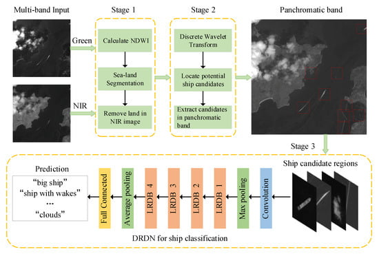
Figure 1.
Workflow of the proposed method based on discrete wavelet transform and the deep residual dense network (DRDN). LRDB, local residual dense block.
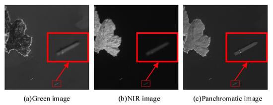
Figure 2.
Three images of different wavebands and resolutions. (a,b) are pixels and have a spatial resolution of 8 m. (c) is pixels and has a spatial resolution of 2 m. All images are scaled to the same size for visualization.
At the sea-land segmentation stage, we utilize the special reflection properties of green and NIR band to separate the sea from the land, i.e., the normalized difference water index (NDWI) [46]. Then, in the ship candidate region extraction stage, DWT is operated on NIR images to highlight all potential ship targets and suppress the undesired backgrounds. Next, we extract all the ship candidate regions in panchromatic images according to the candidate region, locating the results in NIR image and the spatial resolution ratio between the NIR and panchromatic image. Finally, DRDN is designed to verify each ship candidate region as a subclass of ship targets or non-ship targets. More details are described hereinafter.
2.2. Sea-Land Segmentation with Multispectral Images
Sea-land segmentation is an important preprocessing step since there are many ship-like objects on land, as shown in Figure 3. The green circles denote ship-like objects on land, and red circles denote ships at sea. These ship-like objects usually share similar shapes to ships. Instead of using a priori geographic information [14,15] or Otsu segmentation [19] with panchromatic images, we separate the sea from the land with multispectral images due to their different reflection characteristics. As shown in Figure 4, the land surface usually appears darker in the green band than in the NIR band. This is because the terrestrial vegetation has high NIR reflectance, while water has very low NIR reflectance and high green light reflectance. We take full advantage of these special properties and perform sea-land segmentation by NDWI [46].
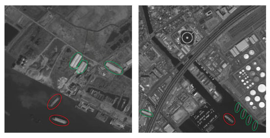
Figure 3.
Some examples of optical remote sensing images. The green circles denote ship-like objects on land, and red circles denote ships at sea. These ship-like objects usually share similar shapes to ships.
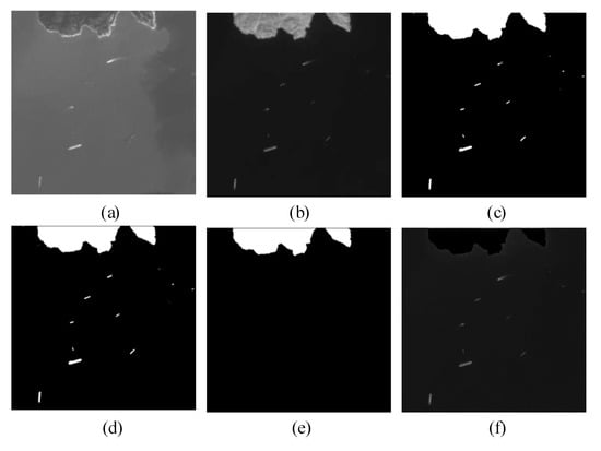
Figure 4.
Sea-land segmentation with multispectral images: (a) green image, (b) NIR image, (c) binarizing with threshold after calculating the NDWI, (d) refined by the morphology closing operation, (e) removing small connected regions at sea, and (f) removing the land area and leaving the sea area in the NIR image.
Given a pair of green waveband image and NIR waveband image , both of size , the NDWI can be calculated as follows:
where and are spatial indexes of the row and column, respectively. According to the above analysis, water area usually has positive values, while land area has zero or negative values. The range of is from −1 to 1. Unlike the binarization method in [17], we employ the reverse binary segmentation. After binarizing with (shown in Figure 4c), we adopt the morphology closing operation to fill the isolated holes (see Figure 4d). Then, the small connected regions are removed if their areas are less than the area threshold t. The land region larger than t is left behind, as shown in Figure 4e. At last, the land regions will be removed in the NIR image according to the bright area in Figure 4e, leaving only the sea area (shown in Figure 4f). The NIR image without land will be used to extract ship candidate regions in the following stage.
2.3. Ship Candidate Region Extraction
Compared with panchromatic images, the sea surface in NIR images is less influenced by illumination or complex weather conditions due to the utilization of the physical characteristics of infrared rays. Hence, we employ NIR images after sea-land segmentation to quickly locate ship candidate regions, not only because of their relatively pure background, but also on account of their relatively low resolution to reduce computational costs. We adopt DWT to extract ship candidate regions due to its advantage of multiresolution analysis, which contributes to singularity detection. After 2D DWT decomposition on the NIR image without land, we gain four groups of frequency coefficients seen as four subimages of size , the low-frequency part and three (horizontal, vertical, diagonal) high-frequency details , , and . Figure 5 shows the four decomposition subimages of Figure 4f. The Haar wavelet basis is adopted to reduce the computational cost.
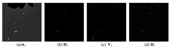
Figure 5.
The decomposition result of Figure 4f based on DWT. (a) denotes the approximation; (b) denotes the horizontal detail image; (c) denotes the vertical low-pass detail image; (d) denotes the diagonal detail image.
As we can see from Figure 5, the bright pixels in , , and describe the image details, e.g., edge variation and distinct points, in different directions (horizontal, vertical, and diagonal). The discontinuities in the spatial domain will lead to local maxima in the wavelet domain [47]. This proves to be effective to detect the singularities by finding these local maxima points [19]. The singularities often carry very important information, and thus, they are particularly useful for object detection. However, these three subimages with resolution reduction only reflect relatively sparse features of the original image. Hence, we enhance the saliency by the formula below:
where , , and represent the interpolation result of , , and . We resize , , and to the size of by the bicubic interpolation algorithm. denotes the enhanced high-frequency detail image. Figure 6 shows the results of the ship candidate region proposal based on enhanced DWT.
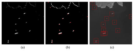
Figure 6.
The results of the ship candidate region proposal based on enhanced DWT. (a) The enhanced high frequency detail image; (b) the centers (red points) of potential ship candidate regions; (c) ship candidate region extraction in the panchromatic image.
The computation steps are as follows.
(1) First, with the purpose of enhancing the contrast between the ship targets and background, , , and are multiplied to obtain , as shown in Figure 6a.
(2) Second, we find each local maximum point in by using a sliding window of size . With respect to the local maxima points, in the region of the sea and land junction, which has a strong response to DWT, we use these local maxima points as centers to spread around and cut square regions of fixed size in Figure 4e.
(3) After that, we calculate the land area in each region and use the value as an auxiliary condition to eliminate the interference of the coastline. Those local maxima points are abandoned if the land areas are above the area threshold t. The potential ship candidate regions are located via the restriction: the number of local maxima. The localization results are shown by red dots in Figure 6b.
(4) With these location points in the NIR images, we can calculate their coordinates in the panchromatic images (of size ) through the proportion of the spatial resolution. The potential ship candidate regions are extracted by the coordinates in the panchromatic images for the following ship classification stage, as shown in Figure 6c.
Note that some ships in the bottom-left of Figure 6b are cut into two parts; however, they are still one target when the candidate regions are extracted in Figure 6c. We end up with multiple candidate regions being extracted for a single target. Although some small response areas in Figure 6b are not detected, these areas correspond to extremely small ships, which are excluded from the target set in our experiments and do not affect the final detection results.
2.4. Ship Classification with DRDN
Recent evidence [33,34] indicates that deeper neural networks can be optimized through skip connections or dense connections, and they can achieve more accurate performance for image classification. ResNet, proposed by He et al. [33], has obtained record-breaking improvements on many visual recognition tasks, which allows identity mapping through deep residual learning to solve the problem of vanishing gradients. To further strengthen feature propagation, Huang et al. [34] introduced by connecting all layers (within the same dense block) directly with each other. This shows that better feature reuse leads to better performance. Inspired by the architectures of ResNet and DenseNet, we design a novel deep residual dense network (DRDN) for ship classification. As shown in Figure 1 (Stage 3), our DRDN mainly consists of four LRDBs and naturally integrates low-/mid-/high-level feature extraction and classifiers in an end-to-end fashion. After obtaining the coordinates of ship candidate regions in panchromatic images, we take these points as centers to spread around and cut them into slices as the input image of DRDN. Then, we extract hierarchical features of ship candidates via a set of LRDBs. The end of DRDN consists of a global average pooling layer and a 10 way fully connected layer with softmax.
Figure 7 illustrates the architecture of LRDB schematically. Our LRDB consists of dense bottleneck layers, the control unit, and the local residual connection. Denote and as the input and output of the k-th LRDB, respectively, and stands for the output of the d-th bottleneck layer in the k-th LRDB. This can be formulated as follows:
where denotes the composite function of three continuous operations: convolution (Conv), batch normalization (BN), and rectified linear unit (ReLU) [48] activation. refers to the concatenation of feature maps produced by the -th LRDB and feature maps produced in Bottleneck Layer 1, …, of k-th LRDB, which results in input feature maps. is the number of feature maps of , and T is known as the growth rate of each bottleneck layer.
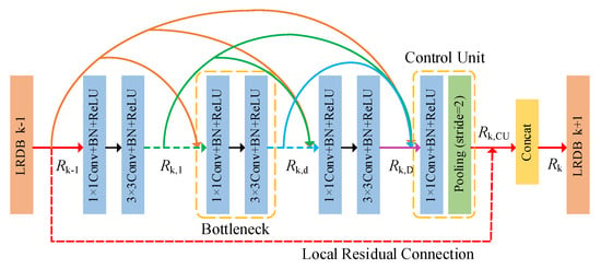
Figure 7.
The architecture of the local residual dense block (LRDB).
Besides dense connections from all preceding layers, we add the control unit to reduce the number of feature maps produced by the preceding LRDB and all the bottleneck layers in the k-th LRDB. The output of the control unit can be obtained by:
To further preserve the feed-forward nature and improve the information flow, we introduce the local residual connection between the -th LRDB and the control unit. The final output of the k-th LRDB is obtained by concatenating and .
We perform downsampling by max pooling with a stride of 2 when the local residual connection goes across feature maps of different sizes. The output of LRDB has direct access to the original input image and dense connections with all preceding layers, which not only maximizes the feature reuse, but also leads to an implicit deep supervision.
3. Dataset and Experiment Setup
3.1. Dataset and Evaluation Metrics
To evaluate the effectiveness of our algorithm, we experiment on twenty panchromatic images and the corresponding multispectral images of the GaoFen-1 satellite, whose wavebands information is detailed in Table 1. These images contain many kinds of landscapes, such as the ocean, the harbor, and the island, which are taken under different light and weather conditions. Since the sizes of satellite images are large, we divide the panchromatic images into with an overlap of 512 pixels and divide the corresponding green and NIR images into with an overlap of 128 pixels. The overlap is to ensure that all ships are intact. The final dataset consists of 2420 groups of images, and each group includes panchromatic, green, and NIR images. All ship targets in panchromatic images are manually labeled as the ground truth information except for some extremely small ambiguous ships. We obtain more than 36,000 ship candidate regions from the above divided images according to the method in Section 2.

Table 1.
Detailed information of GaoFen-1 satellite images.
Based on our observation in the experiment, on the one hand, ship targets among these candidate regions usually have different sizes and moving states. On the other hand, the most common pseudo targets are waves, islands, landing stage, clouds, and so on. To solve the problem of various ship sizes and the huge difference between pseudo targets, we divide these candidate regions into two groups: one is the ship target, and the other is the non-ship target. We manually measure the length of each ship target and artificially divide ship targets into five subclasses according to their length and pixel number along the length: (1) big ship (a length of more than 100 pixels or 200 m), (2) medium ship (a length of about 50–100 pixels or 100 m–200 m), (3) small ship (a length of about 10–50 pixels or 20 m–100 m), (4) multiple ships (many ships docked together), and (5) ship with wakes. Specially, some fuzzy ships (length less than 10 pixels) are excluded from our dataset. Meanwhile, non-ship targets are also divided into five typical categories: (6) waves, (7) islands, (8) landing stage, (9) clouds, and (10) black background. Some typical instances of each class are shown in Figure 8. The quantities of each class are shown in Figure 9.
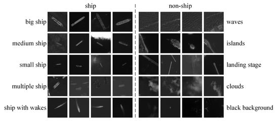
Figure 8.
Some typical instances of ship targets (left) and non-ship targets (right) in our 10 class dataset.
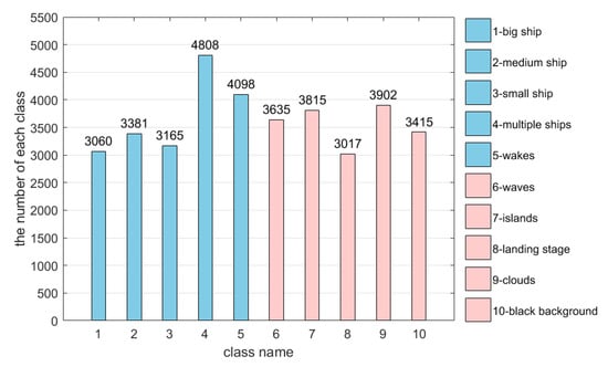
Figure 9.
Distribution of each class in the dataset (36,296 in total).
To quantitatively evaluate the detection algorithm, we employ metrics of precision (P), false alarm rate (F), recall (R), missing rate (M), and F-score. The F-score is used to harmonically average the trade-off between the precision and the recall rate. These criteria are computed as follows:
where , , and respectively stand for the number of accurately recognized ship targets (true positive), the number of non-ship targets misjudged as ships (false positive), and the number of ship targets misjudged as non-ship (false negative). denotes the harmonic mean of the precision and recall rate.
3.2. Implementation Details
In this section, we give concrete implementation details in our experiments. In the sea-land segmentation stage, the land area threshold t is slightly larger than the area of the biggest ship in our dataset. We set it to 800 pixels for 8m resolution multispectral images. In the ship candidate extraction stage, the size of the sliding window L is set to 20. After obtaining the coordinates in the panchromatic images, we use these points as centers to spread around and cut the ship candidate regions into a size of pixels. We randomly select 80% of each category in our 10 class dataset as the training set and the rest as the test set for the ship classification stage.
In our experiment, all candidate regions are subtracted by the per-pixel mean. The data augmentation is adopted at training time: randomly flipping an image and randomly cropping an image padded by 16 pixels to keep the original size. We use 4 residual dense blocks in our DRDN for fair comparison with ResNet and DenseNet. We implement our DRDN with the deep learning framework TensorFlow and update it with the momentum optimizer. DRDN is trained on the 10 class dataset for 100 epochs with a mini-batch size of 32. The learning rate is initialized to 0.01 and drops to its 1/10 every 30 epochs. We use a weight decay of 0.0001. We set T to 32, which denotes the number of feature maps produced by each convolution layer in LRDB. We let the initial convolution layer produce feature maps and each convolution layer in the control unit produce feature maps. Table 2 shows the detailed architectures of DRDN. We design three kinds of DRDN (134 layers, 214 layers, and 278 layers) with different network depths for ship classification. After classification, we calculate the minimum bounding rectangle of each target for precise positioning when the candidate regions are predicted as any subclass of ship targets. In our detection experiment, true positives are those target boxes that have an intersection-over-union (IoU) ratio higher than 0.5 with the ground-truth bounding boxes.
Table 2.
Different DRDN architectures. Note that each Conv layer shown in the table corresponds to the sequence Conv-BN-ReLU.
4. Parameter Setting and Comparative Experiments
4.1. Parameter Setting
At the sea-land segmentation stage, different segmentation thresholds may bring different segmentation effects. We adopt the mean intersection-over-union (mIoU) [49] to measure the separation effects of sea-land segmentation. Let Q denote the mIoU, and its definition is as follows:
where denotes the area of missing segmented land in ground truth images, denotes the area of correctly segmented land by the NDWI algorithm, and denotes the area of wrongly-segmented land by the NDWI algorithm. We choose 726 groups of images with prior geographical information in our dataset to get the ground truth land masks. denotes the area of the ground truth land mask, and denotes the area of the segmented land mask by our algorithm. Because the range of NDWI is (−1,1), we let vary from −1 to 1 at intervals of 0.05 and calculate , , and each time. The mIoU is the average of the above groups. Figure 10 shows the impact of different segmentation thresholds on the mIoU. The closer mIoU is to 1, the better sea-land segmentation will be. We can see from Figure 10 that when is 0.35, the mIoU reaches the maximum value, which is close to 1. Consequently, we set to 0.35 in our experiment.
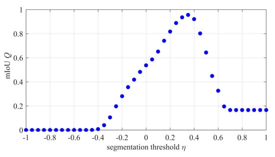
Figure 10.
The impact of different segmentation thresholds on sea-land segmentation. mIoU, mean intersection-over-union.
4.2. Comparisons for Different Sea-Land Segmentation Methods
To verify the effects of sea-land segmentation, we compare the NDWI method in this paper with the common Otsu-based segmentation method. NDWI is calculated with multispectral images, and the Otsu algorithm is operated on the corresponding panchromatic and NIR images. We perform a series of experiments on the 726 groups of images introduced in Section 4.1 and calculate the mIoU of the above three segmentation methods. Table 3 shows the comparative results. The NDWI segmentation algorithm achieves better performance than the Otsu-based methods.
Table 3.
Comparison of the segmentation performance of the NDWI and Otsu-based methods.
Figure 11 shows the sea-land segmentation results on two typical types of land (bright land and dark land). As shown in the first row of Figure 11, the NDWI and Otsu algorithms can both successfully separate the sea from the bright land. As shown in the second row, the Otsu algorithm on panchromatic images (shown in Figure 11f) and NIR images (shown in Figure 11g) divides the dark land incompletely. However, the NDWI algorithm still performs well on dark land (shown in Figure 11h), which demonstrates its robustness.
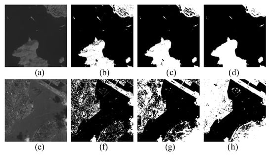
Figure 11.
Sea-land segmentation comparison between Otsu and NDWI. (a,e) denote the original panchromatic images; (b,f) are the results of Otsu on panchromatic images; (c,g) are the results of Otsu on NIR images; (d,h) are the results of NDWI based on NIR and green images.
It is worth mentioning that the proposed segmentation method can separate ships docked on the shore successfully (shown in Figure 12a–e) and eliminate the interference of some bright clouds (shown in Figure 12k–o). As shown in Figure 12c,d, these isolated holes in the land region are filled by the morphology closing operation. Figure 12f–j illustrates the zoom-in version of the red rectangles in Figure 12a–e. These show that the inshore ships will not be removed with the land region, which substantially ensures the accuracy of our next extraction and classification stages.
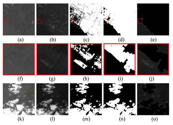
Figure 12.
Sea-land segmentation results under complex backgrounds with inshore ships and bright clouds. (a,k) are green images; (b,l) are NIR images; (c,m) denote sea-land binary segmentation; (d,n) denote removing small connected regions at sea; (e,o) are NIR images without land; (f–j) zoom-in regions of the red rectangles in (a–e).
4.3. Comparisons for Different Classification Strategies
To verify the effectiveness of our multiclass classification strategy, we compare it with the binary classification strategy, which is adopted by many previous detection algorithms [15,17,24]. The binary classification directly treats the ship candidate regions as two categories: ship and non-ship. In the binary classification experiment, for each ship candidate, DRDN-134 (with 2D fully connected layer) is employed to predict whether the object belongs to a ship target or not. However, based on our observation, there usually exists great intra-class difference among the samples within the same class. For instance, in the ship target group, big ships and small ships have different lengths and areas; some ships are static, while some dynamic ships have wakes. This is the same for the non-ship group. These pseudo targets also include many subclasses, such as waves, islands, landing stage, and clouds. All of them have totally different grey distributions and features. The experiments in [16] merely divided ship targets into two categories: big ship and small ship. The samples in [14] were intuitively divided into five typical subclasses: ships, ocean waves, coastlines, clouds, and islands. Zhu et al. [14] did not divide ship samples into multiple subclasses because there were not enough samples. Whereas, it is necessary to divide them into more fine categories for better classification.
In our multiclass classification experiment, we divide the samples into 10 categories and train DRDN-134 with our 10 class dataset. If the candidate sample is predicted as any subclass of the ship targets, the classification result belongs to a ship target. Otherwise, it belongs to a non-ship target. In this experiment, binary classification and multiclass classification are compared, and their results are listed in Table 4. As shown in the table, the precision and recall of binary classification are both lower than those of multiclass classification, which demonstrates the advantages of the multiclass classification strategy. The reason for the poor performance of binary classification is obvious. The ship targets and non-ship targets both have huge intra-class difference while some of their subclasses share similar shapes and features. For example, the clouds and waves have totally disparate texture features and object sizes, while the landing stages and ships may have similar shapes and textures. The multiclass classification finely divides ship targets and non-ship targets into many subclasses and motivates DRDN to learn the abundant and unique features of each category, thus resulting in higher precision and recall.
Table 4.
Ship classification results with different classification strategies.
4.4. Comparisons of Different Classification Networks
To further demonstrate the effectiveness and performance of DRDN on ship classification, we compare our DRDN with state-of-the-art classification networks, especially with ResNet [33] and DenseNet [34]. We adopt 101 layer ResNet and 264 layer DenseNet to compare with our 134 layer DRDN. For a fair comparison, we adopt the same multiclass classification strategy and ensure the same data pre-processing, data augmentation, and other optimization settings. Figure 13 shows the comparison results of the three classification networks. In each subfigure, Numbers 1–5 denote big ship, medium ship, small ship, multiple ships, and ship with wakes, which belong to the ship targets, and Numbers 6-10 denote waves, islands, landing stage, clouds, and black background, which belong to the non-ship targets. The recognition rate denotes the probability of each subclass classified into the 10 classes in the dataset. Different colors indicate the recognition rates of each subclass. The diagonal of the recognition rate matrix stands for the absolutely right classification accuracy.
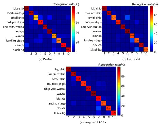
Figure 13.
Recognition rate matrices of different classification networks. Numbers 1–10 in the horizontal axis correspond to the category names in the vertical axis.
The results in Figure 13 show that ResNet, DenseNet, and our DRDN all have high recognition rates for big ships and waves. However, ResNet and DenseNet have lower recognition rates for small ships (in the third row, third column) than our DRDN, which reveals the benefits of the better feature reuse and deep supervision in DRDN. We find that the local residual connection enforces the intermediate layers to extract more discriminative features for different subclasses when comparing our DRDN with DenseNet. Meanwhile, our DRDN also has better classification performance on non-ship targets than ResNet, such as islands and landing stages.
In addition, we design DRDN architectures with different network depths and compare our models with other classification networks, such as AlexNet [32], VGG-16 [50], and Inception V4 [51]. Table 5 summarizes the overall classification performance and model parameters of these networks. As shown in Table 5, the 134/214/278 layer DRDNs are all more accurate than AlexNet and VGG-16. Thanks to the residual connections and dense connections in DRDN, we do not observe the degradation problem and thus enjoy significant accuracy gains by increasing the depth. Compared with ResNet-101, our DRDN-134 has dense connections between layers within one residual dense block, which results in a 5.6% improvement in the F1-measure (precision improved by 5.56%, recall by 5.64%). Compared with DenseNet-264, our DRDN-278 adds local residual connections, and this leads to a 2.91% performance improvement of the measure. Even compared with the powerful Inception V4, our DRDN-278 still shows better precision and recall rates with lower model complexity (32.54 M vs. 41.12 M). All these reveal the advantages of our model design with better feature reuse for ship classification. Considering the real-time requirements of ship detection tasks, we employ DRDN-134 with fewer model parameters as the ship classification network in the following experiments for a better trade-off between accuracy and model complexity.
Table 5.
Performance comparison of different classification networks.
5. Ship Detection Performance Analysis
In this section, the performance of the ship detection algorithm developed in this paper is analyzed.
5.1. Location Performance in Different Image Backgrounds
To further verify the effectiveness of the proposed candidate region extraction method, we conduct experiments with some hard examples like images with mist, strong waves, and complex backgrounds. Figure 14 shows the experimental results. The green ellipses in Figure 14 denote the ground truth of ships, and the red dots denote the centers of potential ship candidate regions. As shown in the third column of Figure 14, all ships under different backgrounds are successfully located by the DWT method in spite of various interferences. Some pseudo targets may be included in the extracted candidate regions. However, they can be removed in the following classification process.
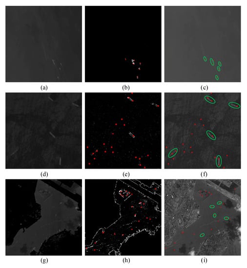
Figure 14.
Ship location performance in different image backgrounds, including images with mist (first row), strong waves (second row), and complex backgrounds (third row). (a,d,g) are NIR images with land removed; (b,e,h) are the enhanced high frequency detail images; (c,f,i) are the localization of potential ship candidate regions on panchromatic images.
5.2. Comparisons with the State-Of-The-Art Detection Methods
We compare our DRDN with traditional detection methods based on hand-crafted features (denoted as CF-SVM) [17], a shallow convolutional network called SVDNet [15], and state-of-the-art end-to-end detection methods SSD [35], YOLOv2 [36], and FPN [38]. SSD is a fast one-stage detector, which introduces the multi-reference and multi-resolution techniques to significantly improve the detection accuracy. It generates scores for the presence of each object category in each default box and produces adjustments to the box to better match the object shape. YOLOv2 is based on the first one-stage detector YOLO [43], which directly predicts bounding boxes, and class probabilities form the entire images in one evaluation. FPN is proposed to build the feature pyramid inside CNNs, which shows great improvement as a generic feature extractor for object detection based on the two stage detector Faster R-CNN [37].
Figure 15 shows the precision-recall curves of different methods. We use the intersections (named break-even point (BEP)) of the black dashed line and precision-recall curves to measure their detection performance. The function of the measurement is . The larger value denotes a better trade-off between the precision and recall rate, which also means higher detection performance. Our DRDN (red curve) clearly outperforms CF-SVM and SVDNet. The main reason is that DRDN extracts more discriminative and abundant features for ship classification, while the hand-crafted features and shallow convolutional neural networks are not strong enough for feature representation. Compared with recent end-to-end detection frameworks SSD, YOLOv2, and FPN, our approach still has outstanding performance, which demonstrates the advantages of our multi-stage design and the sequential elimination process of false alarms. We conjecture that sea-land segmentation may further improve the performance of end-to-end detection methods because the complex land surface usually leads to many false alarms during the detection process.
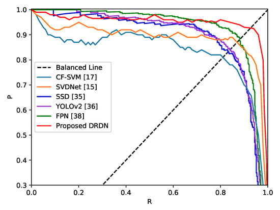
Figure 15.
Precision-recall curves of different ship detection methods. CF-SVM, hand-crafted feature; SSD, single shot multi-box detector; FPN, feature pyramid network.
5.3. Detection Performance in Different Image Backgrounds
In practical applications, optical remote sensing images may be taken under different weather conditions. Figure 16 shows several detection results of some typical environments by our proposed detection framework. We can see that our proposed detection algorithm performs well for quiet seas (see Figure 16a) even though some ships are very small. What is more, due to the multiclass classification strategy, our algorithm could overcome the interference of clouds (see Figure 16b) and waves (see Figure 16c). Even though some ships have long wakes (see Figure 16d) and many ships are docked together (see Figure 16e), we can detect them successfully with our method. Although one ship close to the coast is missed (see the green rectangle in Figure 16e) and there is one false alarm (see the green rectangle in Figure 16f), our detection performance is still very robust and acceptable in these complex environments. One possible solution for these inshore ships is to detect shorelines or harbors first and enhance the accuracy of sea-land segmentation. Improving the detection accuracy of inshore ships will be one of our future works.
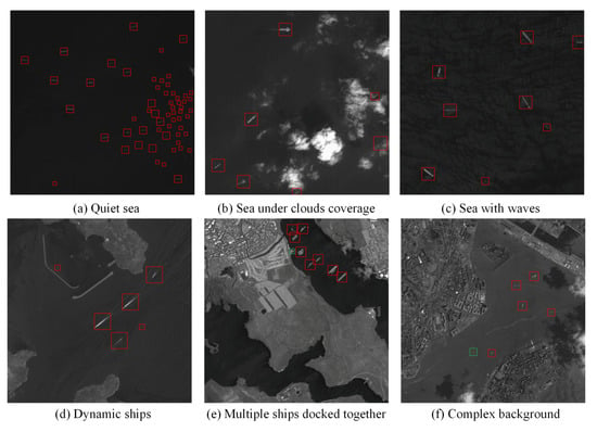
Figure 16.
Ship detection results in different backgrounds. Each image has a size of pixels.
The computational time of the whole algorithm depends on the image contents. Specifically, images with more complex environments will have more ship candidate regions, thus resulting in a longer time. Table 6 shows the time comparison between our DRDN and other CNN-based detection methods. Experiments were performed on a PC with Intel Core i7-8700 CPU@3.7GHz, and an NVIDIA GeForce GTX 1080Ti GPU. Given the same input resolution (), our DRDN runs at a faster speed than SVDNet. Note that, although SSD, YOLOv2, and FPN outperform our method in speed, they have much smaller input resolutions than ours. Consequently, our DRDN achieves a better trade-off between accuracy and speed. The result benefits from fast ship candidate region extraction in the NIR image. Due to the better feature reuse by our DRDN, our method achieves accurate and fast ship detection.
Table 6.
Processing time of different detection methods.
6. Conclusions
In this paper, we propose a novel coarse-to-fine ship detection framework based on DWT and DRDN. Compared with the previous algorithms, we adopt multispectral images to separate sea and land. An enhanced DWT is applied on NIR images for fast ship candidate region extraction, and then, we locate these candidate regions in panchromatic images according to the location results in the NIR image and the spatial resolution ratio between the panchromatic band and the NIR band. In the process of ship classification, DRDN is designed to enhance dense feature fusion and improve the classification accuracy of small objects like ships. In addition, the multiclass strategy is employed to further handle the problem of different ship sizes and interference. Attributed to these contributions, our proposed method can effectively detect both static and moving targets even though ship sizes change greatly. Extensive experiments demonstrate that our scheme performs well in different complex scenes like clouds, waves, and islands and achieves a good trade-off between accuracy and detection speed.
In spite of the overall promising performance, there are still several issues to be further considered. Some targets are missed when inshore ships are adjacent to the land, and shoreline detection or specially-designed convolutional neural networks may be one solution. Our future work will concentrate on improving the detection performance of inshore ships, further reducing false alarms and better exploiting multispectral features.
Author Contributions
L.C. and W.S. conceived of and developed the idea; L.C. performed the experiments; C.F. and L.Z. analyzed the data and helped with the validation; L.C. wrote the paper; D.D. supervised the study and reviewed the paper. All authors have read and agree to the published version of the manuscript.
Funding
This work was supported in part by the National Natural Science Foundation of China (No. 61501334).
Acknowledgments
The authors would like to thank the anonymous reviewers for their valuable comments and helpful suggestions.
Conflicts of Interest
The authors declare no conflict of interest.
References
- Li, H.; Li, Z.; Chen, Z.; Yang, D. Multi-layer sparse coding model-based ship detection for optical remote-sensing images. Int. J. Remote Sens. 2017, 38, 6281–6297. [Google Scholar] [CrossRef]
- Chen, S.; Zhang, J.; Zhan, R. R2FA-Det: Delving into High-Quality Rotatable Boxes for Ship Detection in SAR Images. Remote Sens. 2020, 12, 2031. [Google Scholar] [CrossRef]
- Liang, Y.; Sun, K.; Zeng, Y.; Li, G.; Xing, M. An adaptive hierarchical detection method for ship targets in high-resolution SAR images. Remote Sens. 2020, 12, 303. [Google Scholar] [CrossRef]
- Liu, G.; Zhang, X.; Meng, J. A Small Ship Target Detection Method Based on Polarimetric SAR. Remote Sens. 2019, 11, 2938. [Google Scholar] [CrossRef]
- Fan, Q.; Chen, F.; Cheng, M.; Lou, S.; Li, J. Ship Detection Using a Fully Convolutional Network with Compact Polarimetric SAR Images. Remote Sens. 2019, 11, 2171. [Google Scholar] [CrossRef]
- Lee, K.Y.; Bretschneider, T.R. Improved ship detection using dual-frequency polarimetric synthetic aperture radar data. In Proceedings of the 2011 IEEE International Geoscience and Remote Sensing Symposium, Vancouver, BC, Canada, 24–29 July 2011; pp. 2274–2277. [Google Scholar]
- Zhi, L.; Changwen, Q.; Qiang, Z.; Chen, L.; Shujuan, P.; Jianwei, L. Ship detection in harbor area in SAR images based on constructing an accurate sea-clutter model. In Proceedings of the 2017 IEEE 2nd International Conference on Image, Vision and Computing (ICIVC), Chengdu, China, 2–4 June 2017; pp. 13–19. [Google Scholar]
- Vieira, F.M.; Vincent, F.; Tourneret, J.; Bonacci, D.; Spigai, M.; Ansart, M.; Richard, J. Ship detection using SAR and AIS raw data for maritime surveillance. In Proceedings of the 2016 IEEE 24th European Signal Processing Conference (EUSIPCO), Budapest, Hungary, 29 August–2 September 2016; pp. 2081–2085. [Google Scholar]
- Wang, X.; Chen, C. Ship detection for complex background SAR images based on a multiscale variance weighted image entropy method. IEEE Geosci. Remote Sens. Lett. 2016, 14, 184–187. [Google Scholar] [CrossRef]
- Huang, L.; Liu, B.; Li, B.; Guo, W.; Yu, W.; Zhang, Z.; Yu, W. OpenSARShip: A dataset dedicated to Sentinel-1 ship interpretation. IEEE J. Sel. Top. Appl. Earth Obs. Remote Sens. 2017, 11, 195–208. [Google Scholar] [CrossRef]
- Kang, M.; Ji, K.; Leng, X.; Lin, Z. Contextual region-based convolutional neural network with multilayer fusion for SAR ship detection. Remote Sens. 2017, 9, 860. [Google Scholar] [CrossRef]
- Lin, Z.; Ji, K.; Leng, X.; Kuang, G. Squeeze and Excitation Rank Faster R-CNN for Ship Detection in SAR Images. IEEE Geosci. Remote Sens. Lett. 2018, 16, 751–755. [Google Scholar] [CrossRef]
- Zhou, M.; Jing, M.; Liu, D.; Xia, Z.; Zou, Z.; Shi, Z. Multi-resolution networks for ship detection in infrared remote sensing images. Infrared Phys. Technol. 2018, 92, 183–189. [Google Scholar] [CrossRef]
- Zhu, C.; Zhou, H.; Wang, R.; Guo, J. A novel hierarchical method of ship detection from spaceborne optical image based on shape and texture features. IEEE Trans. Geosci. Remote Sens. 2010, 48, 3446–3456. [Google Scholar] [CrossRef]
- Zou, Z.; Shi, Z. Ship detection in spaceborne optical image with SVD networks. IEEE Trans. Geosci. Remote Sens. 2016, 54, 5832–5845. [Google Scholar] [CrossRef]
- Qi, S.; Ma, J.; Lin, J.; Li, Y.; Tian, J. Unsupervised ship detection based on saliency and S-HOG descriptor from optical satellite images. IEEE Geosci. Remote Sens. Lett. 2015, 12, 1451–1455. [Google Scholar]
- Nie, T.; He, B.; Bi, G.; Zhang, Y.; Wang, W. A method of ship detection under complex background. ISPRS Int. J. Geo-Inf. 2017, 6, 159. [Google Scholar] [CrossRef]
- Van Etten, A. You only look twice: Rapid multi-scale object detection in satellite imagery. arXiv 2018, arXiv:1805.09512. [Google Scholar]
- Tang, J.; Deng, C.; Huang, G.B.; Zhao, B. Compressed-domain ship detection on spaceborne optical image using deep neural network and extreme learning machine. IEEE Trans. Geosci. Remote Sens. 2014, 53, 1174–1185. [Google Scholar] [CrossRef]
- Wu, Y.; Ma, W.; Gong, M.; Bai, Z.; Zhao, W.; Guo, Q.; Chen, X.; Miao, Q. A Coarse-to-Fine Network for Ship Detection in Optical Remote Sensing Images. Remote Sens. 2020, 12, 246. [Google Scholar] [CrossRef]
- Wenxiu, W.; Yutian, F.; Feng, D.; Feng, L. Remote sensing ship detection technology based on DoG preprocessing and shape features. In Proceedings of the 2017 3rd IEEE International Conference on Computer and Communications (ICCC), Chengdu, China, 13–16 December 2017; pp. 1702–1706. [Google Scholar]
- Gan, L.; Liu, P.; Wang, L. Rotation sliding window of the hog feature in remote sensing images for ship detection. In Proceedings of the 2015 IEEE 8th International Symposium on Computational Intelligence and Design (ISCID), Hangzhou, China, 12–13 December 2015; Volume 1, pp. 401–404. [Google Scholar]
- Xu, J.; Sun, X.; Zhang, D.; Fu, K. Automatic detection of inshore ships in high-resolution remote sensing images using robust invariant generalized Hough transform. IEEE Geosci. Remote Sens. Lett. 2014, 11, 2070–2074. [Google Scholar]
- Yang, X.; Sun, H.; Fu, K.; Yang, J.; Sun, X.; Yan, M.; Guo, Z. Automatic ship detection in remote sensing images from google earth of complex scenes based on multiscale rotation dense feature pyramid networks. Remote Sens. 2018, 10, 132. [Google Scholar] [CrossRef]
- Lin, H.; Shi, Z.; Zou, Z. Fully convolutional network with task partitioning for inshore ship detection in optical remote sensing images. IEEE Geosci. Remote Sens. Lett. 2017, 14, 1665–1669. [Google Scholar] [CrossRef]
- Shi, Z.; Yu, X.; Jiang, Z.; Li, B. Ship detection in high-resolution optical imagery based on anomaly detector and local shape feature. IEEE Trans. Geosci. Remote Sens. 2013, 52, 4511–4523. [Google Scholar]
- Li, Z.; Itti, L. Saliency and gist features for target detection in satellite images. IEEE Trans. Image Process. 2010, 20, 2017–2029. [Google Scholar] [PubMed]
- Zhang, R.; Yao, J.; Zhang, K.; Feng, C.; Zhang, J. S-CNN-based Ship Detection from High-Resolution Remote Sensing Images. Int. Arch. Photogramm. Remote Sens. Spat. Inf. Sci. 2016, 41, 423–430. [Google Scholar] [CrossRef]
- Nie, T.; Han, X.; He, B.; Li, X.; Liu, H.; Bi, G. Ship Detection in Panchromatic Optical Remote Sensing Images Based on Visual Saliency and Multi-Dimensional Feature Description. Remote Sens. 2020, 12, 152. [Google Scholar] [CrossRef]
- Yang, F.; Xu, Q.; Li, B. Ship detection from optical satellite images based on saliency segmentation and structure-LBP feature. IEEE Geosci. Remote Sens. Lett. 2017, 14, 602–606. [Google Scholar] [CrossRef]
- Wang, H.; Zhu, M.; Lin, C.; Chen, D. Ship detection in optical remote sensing image based on visual saliency and AdaBoost classifier. Optoelectron. Lett. 2017, 13, 151–155. [Google Scholar] [CrossRef]
- Krizhevsky, A.; Sutskever, I.; Hinton, G.E. Imagenet classification with deep convolutional neural networks. In Proceedings of the Advances in Neural Information Processing Systems 25 (NIPS 2012), Lake Tahoe, NV, USA, 3–6 December 2012; pp. 1097–1105. [Google Scholar]
- He, K.; Zhang, X.; Ren, S.; Sun, J. Deep residual learning for image recognition. In Proceedings of the IEEE Conference on Computer Vision and Pattern Recognition, Las Vegas, NV, USA, 27–30 June 2016; pp. 770–778. [Google Scholar]
- Huang, G.; Liu, Z.; Van Der Maaten, L.; Weinberger, K.Q. Densely connected convolutional networks. In Proceedings of the IEEE Conference on Computer Vision and Pattern Recognition, Honolulu, HI, USA, 21–26 July 2017; pp. 4700–4708. [Google Scholar]
- Liu, W.; Anguelov, D.; Erhan, D.; Szegedy, C.; Reed, S.; Fu, C.Y.; Berg, A.C. Ssd: Single Shot Multibox Detector; European conference on computer vision; Springer: Berlin/Heidelberg, Germany, 2016; pp. 21–37. [Google Scholar]
- Redmon, J.; Farhadi, A. YOLO9000: Better, faster, stronger. In Proceedings of the IEEE Conference on Computer Vision and Pattern Recognition, Honolulu, HI, USA, 21–26 July 2017; pp. 7263–7271. [Google Scholar]
- Ren, S.; He, K.; Girshick, R.; Sun, J. Faster r-cnn: Towards real-time object detection with region proposal networks. In Proceedings of the Advances in Neural Information Processing Systems 28 (NIPS 2015), Montreal, QC, Canada, 7–12 December 2015; pp. 91–99. [Google Scholar]
- Lin, T.Y.; Dollár, P.; Girshick, R.; He, K.; Hariharan, B.; Belongie, S. Feature pyramid networks for object detection. In Proceedings of the IEEE Conference on Computer Vision and Pattern Recognition, Honolulu, HI, USA, 21–26 July 2017; pp. 2117–2125. [Google Scholar]
- Girshick, R.; Donahue, J.; Darrell, T.; Malik, J. Rich feature hierarchies for accurate object detection and semantic segmentation. In Proceedings of the IEEE Conference on Computer vision and Pattern Recognition, Columbus, OH, USA, 23–28 June 2014; pp. 580–587. [Google Scholar]
- Li, K.; Wan, G.; Cheng, G.; Meng, L.; Han, J. Object detection in optical remote sensing images: A survey and a new benchmark. ISPRS J. Photogramm. Remote Sens. 2020, 159, 296–307. [Google Scholar] [CrossRef]
- He, K.; Zhang, X.; Ren, S.; Sun, J. Spatial pyramid pooling in deep convolutional networks for visual recognition. IEEE Trans. Pattern Anal. Mach. Intell. 2015, 37, 1904–1916. [Google Scholar] [CrossRef]
- Girshick, R. Fast r-cnn. In Proceedings of the IEEE International Conference on Computer Vision, Santiago, Chile, 7–13 December 2015; pp. 1440–1448. [Google Scholar]
- Redmon, J.; Divvala, S.; Girshick, R.; Farhadi, A. You only look once: Unified, real-time object detection. In Proceedings of the IEEE Conference on Computer Vision and Pattern Recognition, Las Vegas, NV, USA, 27–30 June 2016; pp. 779–788. [Google Scholar]
- Lin, T.Y.; Goyal, P.; Girshick, R.; He, K.; Dollár, P. Focal loss for dense object detection. In Proceedings of the IEEE International Conference on Computer Vision, Honolulu, HI, USA, 21–26 July 2017; pp. 2980–2988. [Google Scholar]
- Li, X.; Wang, S.; Jiang, B.; Chan, X. Inshore ship detection in remote sensing images based on deep features. In Proceedings of the 2017 IEEE International Conference on Signal Processing, Communications and Computing (ICSPCC), Xiamen, China, 22–25 October 2017; pp. 1–5. [Google Scholar]
- McFeeters, S.K. The use of the Normalized Difference Water Index (NDWI) in the delineation of open water features. Int. J. Remote Sens. 1996, 17, 1425–1432. [Google Scholar] [CrossRef]
- Tello, M.; López-Martínez, C.; Mallorqui, J.J. A novel algorithm for ship detection in SAR imagery based on the wavelet transform. IEEE Geosci. Remote Sens. Lett. 2005, 2, 201–205. [Google Scholar] [CrossRef]
- Glorot, X.; Bordes, A.; Bengio, Y. Deep sparse rectifier neural networks. In Proceedings of the Fourteenth International Conference on Artificial Intelligence and Statistics, Fort Lauderdale, FL, USA, 11–13 April 2011; pp. 315–323. [Google Scholar]
- Long, J.; Shelhamer, E.; Darrell, T. Fully convolutional networks for semantic segmentation. In Proceedings of the IEEE Conference on Computer Vision and Pattern Recognition, Santiago, Chile, 7–13 December 2015; pp. 3431–3440. [Google Scholar]
- Simonyan, K.; Zisserman, A. Very Deep Convolutional Networks for Large-Scale Image Recognition. arXiv 2014, arXiv:1409.1556. [Google Scholar]
- Szegedy, C.; Ioffe, S.; Vanhoucke, V.; Alemi, A.A. Inception-v4, inception-resnet and the impact of residual connections on learning. In Proceedings of the Thirty-first AAAI Conference on Artificial Intelligence, San Francisco, CA, USA, 4–9 February 2017. [Google Scholar]
© 2020 by the authors. Licensee MDPI, Basel, Switzerland. This article is an open access article distributed under the terms and conditions of the Creative Commons Attribution (CC BY) license (http://creativecommons.org/licenses/by/4.0/).