Article

Use of Visible and Near-Infrared Reflectance Spectroscopy Models to Determine Soil Erodibility Factor (K) in an Ecologically Restored Watershed

1
Key Laboratory of Aquatic Botany and Watershed Ecology, Wuhan Botanical Garden, Chinese Academy of Sciences, Wuhan 430074, China
2
School of Resource and Environmental Science, Wuhan University, No.129 Luoyu Road, Wuhan 430079, China
3
China Railway Fifth Survey and Design Institute Group Co., Ltd., Beijing 102600, China
*
Author to whom correspondence should be addressed.
Remote Sens. 2020, 12(18), 3103; https://doi.org/10.3390/rs12183103
Submission received: 26 August 2020 / Revised: 21 September 2020 / Accepted: 21 September 2020 / Published: 22 September 2020

Abstract

:
This study aimed to assess the ability of using visible and near-infrared reflectance (Vis–NIR) spectroscopy to quantify soil erodibility factor (K) rapidly in an ecologically restored watershed. To achieve this goal, we explored the performance and transferability of the developed spectral models in multiple land-use types: woodland, shrubland, terrace, and slope farmland (the first two types are natural land and the latter two are cultivated land). Subsequently, we developed an improved approach by combining spectral data with related topographic variables (i.e., elevation, watershed location, slope height, and normalized height) to estimate K. The results indicate that the calibrated spectral model using total samples could estimate K factor effectively (R2CV = 0.71, RMSECV = 0.0030 Mg h Mj−1 mm−1, and RPDCV = 1.84). When predicting K in the new samples, models performed well in natural land soils (R2P = 0.74, RPDP = 1.93) but failed in cultivated land soils (R2P = 0.24, RPDP = 0.99). Furthermore, the developed models showed low transferability between the natural and cultivated land datasets. The results also indicate that the combination of spectral data with topographic variables could slightly increase the accuracies of K estimation in total and natural land datasets but did not work for cultivated land samples. This study demonstrated that the Vis–NIR spectroscopy could be used as an effective method in predicting K. However, the predictability and transferability of the calibrated models were land-use type dependent. Our study also revealed that the coupling of spectrum and environmental variable is an effective improvement of K estimation in natural landscape region.

Graphical Abstract

1. Introduction

Soil erosion is a severe eco-environmental issue worldwide that threatens sustainable land utilization and ecosystem stability [1,2,3]. It causes serious off-site pollution in channels and reservoirs, thereby reducing their storage volume, lifetime, and ecological benefits [4,5]. The analysis and quantification of soil erosion and its linked processes are essential for the conservation of natural resources [6]. Soil erodibility reflects the inherent susceptibility of soil to exogenic erosive forces, and it is one of the key parameters for estimating soil loss [7,8]. However, the direct field measurement of soil erodibility is costly, time-consuming, and method-dependent [9]. Therefore, pedotransfer functions have been adopted as alternatives, to estimate soil erodibility using easily measurable basic soil properties [10]. In the past decades, the Universal Soil Loss Equation (USLE) and revised USLE (RUSLE) were the two most widely used empirical equations for erosion prediction [11]. In these models, soil erodibility (introduced as the K factor) is calculated by using several soil properties, including particle size composition, soil organic carbon (SOC) content, structural stability, soil permeability, and clay minerals [12]. To accurately measure these properties, field soil samplings and laboratory analyses are necessary, which are labor intensive, time-consuming, and expensive. Furthermore, for a given soil, K factor changes with the expansion of space and variation of seasons [13], which further complicate the estimation of K factor. Thus, a reliable, fast, and economic measuring method is needed to assess K factor.
Visible and near-infrared reflectance (Vis–NIR) spectroscopy is a promising alternative to the conventional methods used for determining soil properties [14]. Vis–NIR spectroscopy has been proven to be an easy, fast, nondestructive, and low-cost soil analytical technique [15]. Moreover, several soil properties can be measured simultaneously from one spectral scan [16,17]. The intrinsic optical properties caused by the compositional and structural information of molecules (e.g., chemical bonds O-H, C-H, C=O, N-H, and/or their combination) can be reflected as the distinct absorption features over the spectral wavelengths of 350–2500 nm [16,18]. A range of soil properties, including SOC, total nitrogen, iron oxide, CaCO3, and soil texture, have been successfully estimated in many studies based on these spectral features [19,20,21].
K factor is determined by the physical and chemical properties of soil, which interacts in complicated ways to produce a specific spectrum. Few studies have utilized spectral reflectance data to predict K factor [22,23,24]. Among these studies, the prediction accuracies were widely variable from unsatisfactory to satisfactory. Thus, it is necessary to evaluate the ability of Vis–NIR spectroscopy in estimating soil K and to explore the possible reasons for the diverse performances. In general, most of the models are location-dependent and data-specific [25,26]. The source of the Vis–NIR (or soil properties) data together with their statistical characteristics could influence the performance of developed assessment models significantly [18]. Frequently, successful prediction results are obtained when homogeneous samples with adequate soil variability of the target site are analyzed [25,27]. However, large bias exists when predicting heterogeneous samples because of the large differences in soil property and spectra [28]. In different land-use types, the soil parent materials, land cover, and range of the K factor values might vary [13]. If all the derived models do not contain the spectral diversity from a new certain (target) site, then it begs another question: Will a model calibrated from samples in a certain land-use type work in other landscape soils? In other words, can a spectral model calibrated in a specific land-use type be transferred to other conditions? Thus, studies concerning the Vis–NIR spectroscopy estimation of the surface K factor with samples from different land-use types should be conducted.
In recent decades, numerous efforts have been made to develop efficient spectral pre-processing and noise-canceling techniques and multiple calibration methods [29,30,31], such as multiple linear regression (MLR), partial least-squares regression (PLSR), artificial neural networks (ANN), and support vector machine (SVM), to improve the analytical ability of the calibrated spectral model. However, these techniques were only conducted from the perspective of spectroscopy, statistics, and chemometrics methods and did not consider the relationships between soil and environment factors. Considering that soil properties were strongly affected by parent material and environmental conditions, the use of spectral data combined with the assistance of environmental factors is expected to generate more accurate predictions. However, no such study that coupled the Vis–NIR spectral data and related auxiliary variables is available to predict K factor. In mountain areas with strong soil erosion, topography is the key factor that controls the spatial distribution of physical and chemical properties of soil [32]. Thus, we hypothesized that topographic factors are important variables that affect K factor. If this hypothesis is true, then the prediction model of K could be improved significantly by incorporating topographic variables.
The Danjiangkou Reservoir is the water source of China’s South-to-North Water Diversion Project-Middle Route. Several decades ago, the watershed that surrounded the reservoir was seriously damaged with problems including water erosion, nutrient loss, and soil degradation [33]. Since the 1980s, a series of ecological restoration measures, such as the “Grain for Green” and “Land Consolidation” programs, has been conducted to prevent soil erosion [34]. In these projects, large areas of undesirable lands, such as bare land and slope farmland, have been converted into woodland, shrubland, or terraces. Meanwhile, the surface soil characteristics have also been changed significantly because of these restoration practices. In this area, K factor, which suffers from complex topography and intense human disturbance, exhibited strong spatial heterogeneity [35]. This instance made the monitoring of the soil’s K factor difficult, especially over large areas and across different land-use types. Therefore, the potential of using Vis–NIR spectroscopy to estimate soil K, which may provide an effective method for quick and economic soil erosion monitoring, should be assessed.
This study aimed to evaluate the effectiveness of using Vis–NIR spectral model to predict K factor in a restored watershed with different land-use types. Specifically, we aimed to assess the performance of Vis–NIR spectral model to quantify soil K factor in a representative ecologically restored watershed rapidly, explore the transferability of the developed models among different land-use types, and develop an improved approach that combined the Vis–NIR spectral data with related topographic variables to estimate K factor better. We hypothesized that the inclusion of topographic variables would improve model performance in estimating soil K factor significantly.

2. Materials and Methods

2.1. Study Area and Sampling

The study was carried out in a typical ecologically restored watershed (32°45′ N, 111°13′ E) around the Danjiangkou Reservoir in Central China (Figure 1). The watershed is characterized by hilly land with an area of 1.92 km2, and elevation range of 277–379 m a.s.l. The climate in this area is subtropical monsoon with an average annual temperature of 15.7 °C, and the average annual precipitation of 973 mm [36]. The soil types in this watershed, according to USDA Soil Taxonomy, are Inceptisols and Alfisols, which correspond to purple soil and yellow-brown soil (Chinese soil classification system), respectively. Terrace farmland and woodland are the two main land-use types, followed by shrubland and slope farmland. Based on our surveys, the upper- and mid-watershed regions are mainly covered by coniferous plants (Platycladus orientalis (Linn.) Franco) and shrub-land plants (Sophora davidii (Franch.) Skeels). Terrace and slope farmlands are mostly located in the mid- and lower-watershed regions; the typical crops in this area include rape, corn, and wheat.
In total, 138 surface soil samples were collected using a 5.0-cm diameter auger in the spring of 2017 and 2018. The number of samples for each land-use type was determined on the basis of their relative area. At representative land-use types, soil samples were randomly collected. Terrace, woodland, shrubland, and slope farmland had 64, 43, 20, and 11 samples, respectively (Figure 1). At each site, approximately 1.0 kg of soil sample was collected. The geographic positions of the sampling sites were recorded using a portable GPS.

2.2. Soil Properties and Environmental Variables

The 138 soil samples were air-dried, sieved with a 2-mm sieve, and analyzed for soil texture and organic carbon content. Soil bulk density (BD) was determined using 100 cm3 soil cores extracted from each of the locations. Soil pH was measured with a calomel electrode (Mettler Toledo FE20, SWIT). SOC content was determined by an elemental analyzer (Thermo Fisher Flash 2000, Waltham, MA, USA). Soil texture (clay, <0.002 mm; silt, 0.002–0.02 mm; and sand, 0.02–2 mm) was measured by laser diffraction method with a Mastersizer 3000 laser diffraction particle size analyzer (Malvern Instruments, Malvern, UK).
The soil erodibility factor K values of the collected samples were determined using the widely used equation in Erosion/Productivity Impact Calculator model (EPIC) [37]. In the Danjiangkou Reservoir region, the rationality and validity of this model in K value estimation have been reported in previous literature [33]. In this model, the particle-size composition and SOC content were used to calculate the algebraic approximation of K:
K = { 0.2 + 0.3 exp [ 0.0256 S d ( 1 S i 100 ) ] } × S i Cl + S i 0.3 × [ 1 0.25 C C + exp ( 3.72 2.95 C ) ] × [ 1.0 0.7 SN SN + exp ( 5.51 + 22.9 SN ) ]
where K is the soil erodibility (Mg h Mj−1 mm−1); S d , S i , and Cl are the percentages of sand, silt, and clay, respectively; C is the percentage of SOC; and S N = 1 S d / 100 . Finally, the equation results were divided by 0.1318 and converted to the standard international units (i.e., Mg h MJ−1 mm−1) [33].
The topographic variables were extracted from the global digital elevation model (DEM) dataset (with 30 m × 30 m spatial resolution) as auxiliary variables to predict K factor. Particularly, the slope position means a relative Euclidean distance from ridgeline, while the watershed location indicates a ratio of the distances from the northern boundary to the longest watershed length in the south–north direction. Elevation (m), slope (degree), slope position (percent), and watershed location (percent) were determined using the ArcGIS 10.2 software (ESRI Inc., Redlands, CA, USA). The topographic indicators, including topographic position, topographic wetness index, slope height (m), and normalized height, were calculated using SAGA GIS 7.2.0 software [38].

2.3. Spectra Measurements and Pre-Processing

The reflectance spectrum of soil samples was measured in a dark room at night using an ASD FieldSpec® Pro FR spectrometer with wavelength of 350–2500 nm. A 50-W halogen lamp with an incident angle of 45° and at a distance of approximately 0.50 m from the sample surface was used as the light source [39]. The spectral data were collected through a fiber probe, which was located in a nadir position with a distance of 15 cm from the sample. Each soil spectrum was obtained as a mean value of 10 replicate scans and was converted to the reflectance values using a standardized Spectralon panel (Labsphere, www.labsphere.com) as the white reference [31].
Before developing K factor prediction models, data pretreatments, including the Savitzky–Golay smoothing, standard normal variate transformation, and mean centering, were performed to reduce noise and enhance spectral features in the MATLAB version 2013a (The MathWorks Inc., Natick, MA, USA). Spectral data with high signal-to-noise ratio (at the wavelength of 400–2350 nm) were used for model calibration.

2.4. Statistical Analyses and Modeling

The descriptive statistics and Pearson correlation analyses were first implemented using MATLAB 2013a. We adopted the three-level interpretations of coefficient of variation (CV) [40]: most variable (with CV > 35%); moderately variable (with 15% < CV < 35%); and least variable (with CV < 15%). One-way analysis of variance (ANOVA) with Tukey’s multiple comparison test (HSD) was performed to examine the effects of land-use types on K factors. The ANOVA was performed using IBM SPSS Statistics 21.0 software. The Pearson correlation coefficient with a confidence level of 99.99% (two-tailed) was used to assess the relationships between the spectra and the K factors and link the soil properties. Then, partial least-squares regression (PLSR) method was used to establish relations between the preprocessed spectra with the K factors. PLSR method is a mainstream modeling technique used for the quantitative analysis of Vis–NIR spectra, mainly because of its superiority in reducing dimensionality of spectral matrix and avoiding multicollinearity [17,27]. Three PLSR modeling strategies were conducted to achieve the objectives of this study:
(1) Calibration and cross-validation. All samples were first split into seven datasets according to land use types (i.e., total samples, natural land, cultivated land, woodland, shrubland, terrace, and slope farmland datasets). Among them, the natural land dataset was the union of woodland and shrubland datasets, whereas the cultivated land dataset was the combination of terrace and slope farmland datasets. All of the samples were united into the total sample datasets. Then, PLSR calibration model with spectrum was developed for each dataset. The leave-one-out cross-validation was conducted to determine the optimum latent variables (LVs) for each PLSR model.
(2) External-validation and transferability evaluation. For each dataset, the samples were separated into a training dataset (with two-thirds of the samples) and a test dataset (with the remaining one-third) using the Kennard–Stone algorithm [41]. The training dataset was used to calibrate the PLSR model, and the test dataset was used to evaluate the predictive capacity of the model for K estimation. To examine the transferability of the Vis–NIR PLSR models among different land-use types, each calibration model was assessed with each test dataset to evaluate its transferability among different land use types.
(3) Optimization with topographic variables and external validation. Topographic variables were combined with the Vis–NIR spectral data to optimize modeling. First, Pearson correlation analyses between the K factor and topographic variables were implemented, and the significant variables were selected to be incorporated into the model to predict K factor. The PLSR model was calibrated on the basis of the training dataset from the total sample datasets, and the test dataset was used for validation. Before modeling, all topographic variables were standardized to solve the problem of non-uniform units.
In addition, the important reflection wavelengths in predicting K factor were determined by the variable importance in the projection (VIP) and PLSR regression coefficients (i.e., b-coefficients). The wavelengths that have large VIP score (>1) and large coefficient value (>standard deviation of the K factor values) are considered important [42]. Predictive performance of a model was assessed by the coefficient of determination (R2), root mean square error (RMSE), and residual prediction deviation (RPD). In general, the model with relatively high R2 and RPD values and small RMSE was considered a better model. Specifically, for the Vis–NIR estimation of the soil properties, R2 > 0.5 and RPD > 1.4 indicate an acceptable predictability (i.e., a good transferability) for the model [43].

3. Results

3.1. Description Statistics of Soil, Topographic Variables, and Spectral Property

The chemical and physical properties of soil exhibited a wide range of variation (Table 1). Soil texture showed a moderate variability (with CVs of 16.93–33.45%) and a wide range: clay content ranged from 4.33% to 34.64%, silt content ranged from 22.35% to 70.26%, and sand content ranged from 15.02% to 73.32%. The mean values of all soil properties were similar to those of the median values. The soil pH of this study area ranged from 5.37 to 8.64 with a mean value of 8.09, thereby suggesting the slight alkalinity for most of the soil samples. SOC had a mean value of 7.61 g kg−1 with a range of 2.49–18.65 g kg−1. SOC had the highest variability with the CV of 49.67%, whereas the CVs of pH, bulk density, and K factor were 7.27%, 12.02%, and 13.10%, respectively (Table 1). Most soil properties were approximately normally distributed on the basis of the skewness and kurtosis values. Only pH was non-normal distributed (with the skewness of −2.69 and kurtosis of 10.30).
In Table 1, the measured K factors varied from 0.027 to 0.057 Mg h Mj−1 mm−1. Significant differences were observed in K factors between natural and cultivated land, and among the four land-use types (Figure 2). Natural land had a significantly lower K value than cultivated land. However, its variation was higher. Soil K factor in woodland was significantly lower than the three other land-use types, but its variation was the highest. Shrubland, terrace, and slope farmland had comparable K values, whereas the variations in K followed the rank of shrubland > terrace > slope farmland.
Table 2 shows the result of the statistical analysis of the topographic variables that may influence K. The slope position and watershed location varied from 1.53% to 99% and from 0.64% to 96.54%, respectively. The CV values for the slope position and watershed location were 60.40% and 47.34%, respectively. The mean elevation was 313.98 m and the mean slope was 5.45°, indicating that the terrain of our study area consisted of mountains and hills of low elevation and gentle slope. Moreover, the CVs of the elevation and topographic wetness index were 7.40% and 31.71%, respectively. The CVs of slope, slope height, normalized height, and topographic position index were quite large (with values of 101.37%, 80.69%, 49.50%, and 438.96%, respectively).
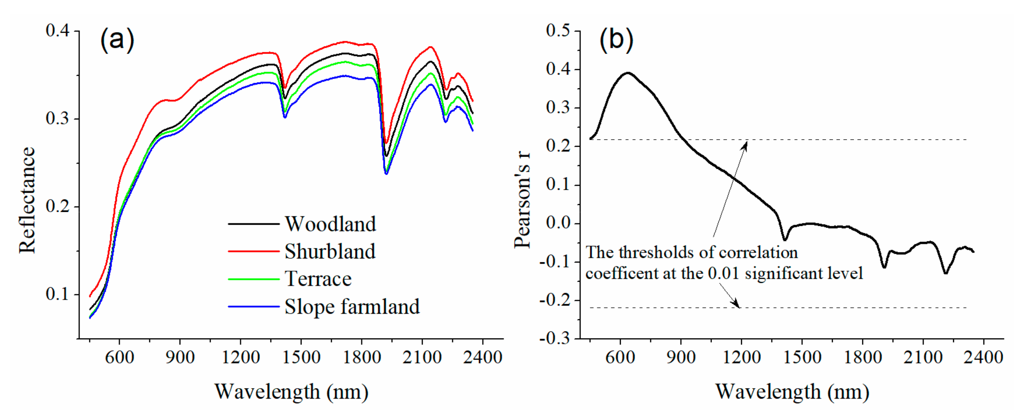
Figure 3a illustrates the effects of land use type on spectral reflectance. The spectral reflectance characteristics were similar among different land use types across the full range of wavelength. In particular, reflectance in the visible wavelength region increased with wavelength, and three specific absorption bands around 1400, 1900, and 2200 nm were presented in the near-infrared wavelengths. The average soil spectrum of shrubland has the highest reflectance, followed by woodland, terrace, and slope farmland. Soil K factor and the reflectance spectra had significant correlations in the visible wavelength region at the 0.01 significance level (Figure 3b). These relationships implied the possibility in estimating K factor using the Vis–NIR spectra.

3.2. Model Calibration Using PLSR Method

The calibration results of the PLSR models in estimating soil K are presented in Table 3. Wide variations in the cross-validation accuracies of Vis–NIR spectral models for the seven different datasets were observed. For the total samples, the calibrated PLSR model can effectively estimate the K factor with R2CV value of 0.71, RMSECV value of 0.0030 Mg h Mj−1 mm−1, and RPDCV value of 1.84. The PLSR model for natural land achieved better cross-validated accuracies than that for the cultivated land. In particular, the best cross-validation result was achieved by using the natural land dataset (R2CV = 0.79, RMSECV = 0.0029 Mg h Mj−1 mm−1, and RPDCV = 2.20) followed by the woodland (R2CV = 0.74, RPDCV =1.99) and shrubland datasets (R2CV = 0.62, RPDCV =1.56). By contrast, calibrations that use cultivated land datasets failed to generate acceptable models to predict soil K factors (R2CV = 0.19–0.46, RPDCV = 0.96–1.32).
Figure 4 illustrates the important wavelengths for K factor monitoring based on VIP and b-coefficient over the entire wavelength range (400–2350 nm). According to these two indicators, the wavelengths centered near 468, 1408, 1899, 1932, 2207, and 2300 nm were identified as the optimal wavelengths for K estimation.

3.3. Performance and Transferability of PLSR Models

In this study, R2P and RPDP values were used to assess the performance and transferability of PLSR models in estimating K. The index matrices of these values are mapped in Figure 5. The colors scaled from dark red for high values to dark blue for low values, where the higher values indicate stronger transferability.
Figure 5 shows that the Vis–NIR spectra performed well in predicting the soil’s K factors for the total sample (R2P = 0.59 and RPDP = 1.52), natural land (R2P = 0.74 and RPDP = 1.93), and woodland (R2P = 0.61 and RPDP = 1.57) datasets. The prediction accuracy of the model for shrubland soil dataset was marginally acceptable (R2P = 0.45 and RPDP = 1.34). However, for the cultivated land dataset, the prediction accuracy was not acceptable (R2P of 0.22–0.92 and RPDP of 0.97–1.01).
Moreover, the transferability results of the PLSR models were quite variable. Similar to the cross-validation results, most of the PLSR models could be transferred (RPDP > 1.4, R2P > 0.5) within the natural land datasets (i.e., natural land dataset, woodland dataset, and shrubland dataset). Especially, the calibrated PLSR model using natural land dataset could predict the K factors of the shrubland sample dataset (with R2P of 0.92, and RPDP of 2.82) satisfactorily. However, the models for the cultivated land datasets (i.e., cultivated land, terrace, and slope farmland datasets) showed low transferability (with RPDP < 1.4, R2P < 0.5). In addition, R2P matrices (in Figure 5a) showed a greater difference in colors than the RPDP matrices (Figure 5b), especially for the slope farmland dataset (n = 11).

3.4. Performance of the Improved Models

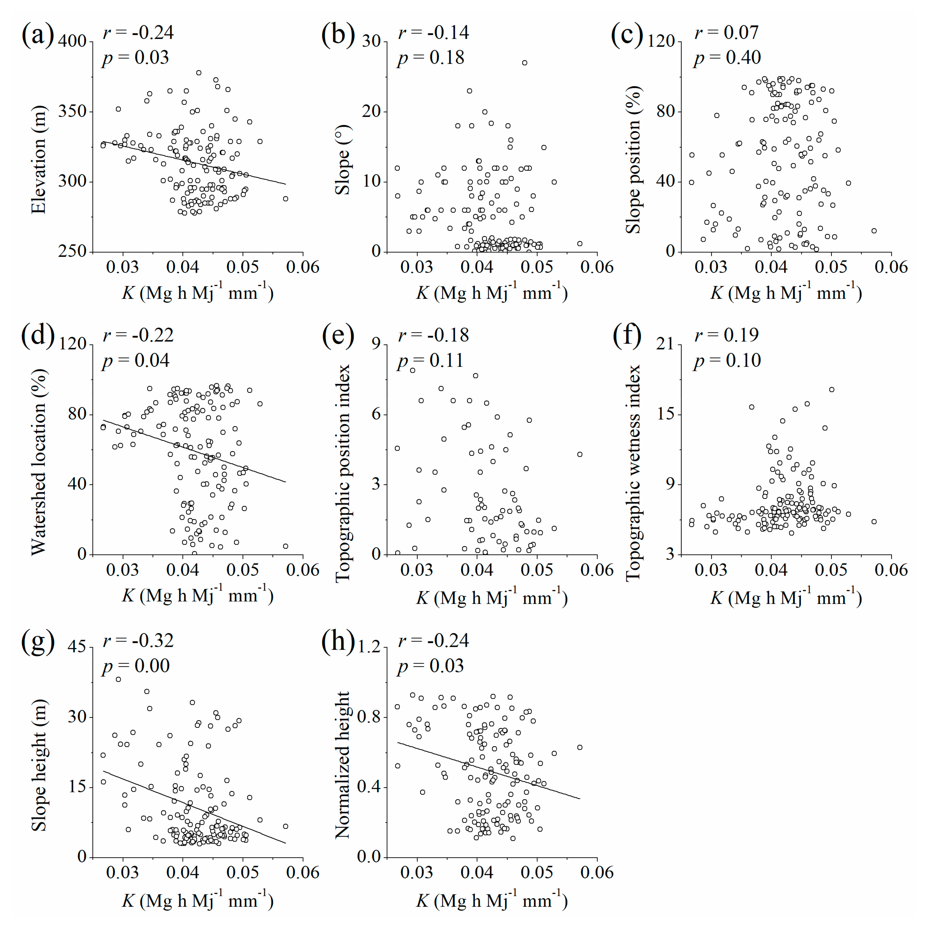
Pearson’s correlation was used to analyze the relationships between the topographic characteristics and K factor. As presented in Figure 6, K factor showed significant negative correlations with elevation (r = −0.24, p = 0.03), watershed location (r = −0.22, p = 0.04), slope height (r = −0.32, p = 0.00), and normalized height (r = −0.24, p = 0.03). However, other topographic characteristics (i.e., slope, slope position, topographic position index, and topographic wetness index) have no significant relationships with K factor (p > 0.05). We attempted to develop an optimized model using the significant correlated topographic variables in combination with the Vis–NIR spectral data to improve the prediction accuracies of K factor.
Figure 7 summarizes the performance of the initial and improved PLSR models to predict K factor. In contrast with the initial model (R2P = 0.59 and RPDP = 1.52), the improved model that used total samples provided a higher accuracy in K factor estimation (R2P = 0.69 and RPDP = 1.78). However, model improvements for different land-use types showed a marked difference. In particular, the improved model could strengthen the prediction accuracy for natural land samples (R2P increased from 0.74 to 0.78 and RPDP increased from 1.93 to 2.07) but had no or little effect on cultivated land datasets (R2P changed from 0.24 to 0.15 and RPDP changed from 0.99 to 1.02).

4. Discussion

The results indicate that the PLSR model calibrated using the total sample dataset (n = 138) could estimate soil K effectively. The model achieved a fairly satisfactory result (R2P = 0.59 and RPDP = 1.52) when the model was applied to new samples, thereby showing reliable predictability. These results are consistent with a previous study [9], in which the PLSR model also performed fairly well (R2 = 0.56 and RPD = 1.5) in estimating the K factor based on reflectance spectroscopy. Land use type showed a strong effect on the performance of PLSR models. PLSR models developed for natural land datasets (e.g., natural land, woodland, and shrubland datasets) generally performed better than models from cultivated land datasets (e.g., cultivated land, terrace, and slope farmland), indicating that human disturbance and cultivation disrupted the relationship between soil properties and its spectroscopy. In comparison, the best cross- and external-validation results were found in woodland samples followed by the shrubland dataset. Both datasets achieved relatively good or acceptable predictability in predicting new samples. The prediction accuracies for the terrace and slop farmland datasets cannot reach the application level. These contrasting results might be attributed to the specific data characteristics. Previous researchers showed that the source of data together with its statistical characteristics could influence model performance significantly [18]. Moreover, a larger size of calibration dataset with bigger CV values should be more beneficial for the robust Vis–NIR estimation of soil properties [18,25,39]. In this study, the CV values of total samples and natural land datasets were relatively bigger (11.68–16.16%) than cultivated land datasets (4.07–8.30%), thereby achieving better prediction accuracies.
When the calibrated PLSR models were used to predict the K factor in other different land-use samples, the prediction accuracy changed remarkably, as shown by heterogeneous color matrices in Figure 5. The results clearly show that the calibrated models for K factor estimation were not transferable between the natural and cultivated land datasets. This result may reinforce the previous implication that the source and quality of the data determine the transferability of model in the prediction of new soil properties. In this study, the heterogeneous soil characteristics of different land-use types presented inadequate spectral diversity of the target site soils and therefore could not be used for the successful prediction [28]. Generally, the constructed soil spectral calibration models should contain the variability of the target site soils on which the models are to be used reasonably [19,44]. However, this premise is not always easy to implement. To solve this problem, researchers proposed the development of a model with spiking, including a few samples from the target sites and subsequent recalibration, which could improve model performance in transferability greatly [28]. Thus, in future studies, the spiking approach should be explored to improve the applicability of spectral models in predicting K factors from different land-use types. Moreover, R2P matrices (Figure 5a) showed remarkable differences at colors scaled in comparison with RPDP matrices (Figure 5b), especially for the slope farmland samples (n =11) as the validation dataset. This finding reinforces that the models developed from relatively smaller size of datasets were more vulnerable to the variation in the data distribution and thus suffered from inconsistent results [18,28]. Therefore, a robust calibration dataset with appropriate sample size would be better for the estimation of K factor using the Vis–NIR spectra.
In this study, the wavelengths centered near 468, 1408, 1899, 1932, 2207, and 2300 nm were identified as the optimal wavelengths for K factor estimation. Generally, soil spectral reflectance is mainly influenced by particle size distribution, SOC content, CaCO3 content, and pH [17,45]. Previous studies indicated a decrease in reflectance with the increase in particle size, SOC content, and CaCO3 content [9]. Such properties interact with one another and display the distinct spectral reflectance features over the spectral wavelengths of 400–2350 nm. Babaeian et al. (2015) stated that SOC exhibited absorption bands in the visible region [46]. Islam et al. (2003) also reported that 350–700-nm bands could be used better for SOC prediction [45]. The reflectances near 1408 and 2207 nm were related to the clay mineral kaolinite [47], whereas the wavelengths near 2206 and 2300 nm were mainly caused by the reflection of illite [48,49]. In addition, the reflectances near 1899 and 1932 nm could be identified as the spectral feature of clay content in air-dried soil because of the strong moisture absorption of soil clay particles [26]. Except for the 468-nm wavelength, most of the identified important wavelengths were within the near-infrared spectra region (>1400 nm), which are mentioned above as the response bands of soil particle size distribution. Therefore, soil texture (i.e., the clay, silt, and sand contents) seems to have played a more important role than the SOC content in the prediction of K factor using Vis–NIR spectral data.
Our study also found that the incorporation of topographic variables into the PLSR model could conditionally increase the prediction accuracy of K factor in the total dataset. However, the improvement was limited. This phenomenon is mainly because of the low correlations (r values varied from −0.32 to −0.22) between the K factor and the topographic characteristics (Figure 6). When considering land-use types, K factor estimation performance improved in the natural land dataset, but no substantial improvement was observed in the cultivated land samples. These different results may be ascribed to the inherent relationships between soil and topography. On the one hand, the rough spatial resolution (30 m × 30 m) may blur the possible correlations between the K factor and the topographic characteristics. On the other hand, as a typical restored watershed, the intensive human activities have greatly altered the local soil, plants, and even geomorphology, especially for the terrace, in which the original correlation between soil and topography was inevitably weakened. Consequently, the topographic factors had no significant role in the improved model that used cultivated land dataset. Based on this finding, we suggest that the Vis–NIR spectra of soil combined with topographic variables can be used to predict K factor in natural landscape region with no significant artificial disturbance, while, for the cultivated land, the different crop types, agronomic practices, and management styles should be considered when optimize modeling.
In this study, there were two major limitations for using Vis–NIR spectral model to estimate soil K factor. Firstly, the predictability of the constructed spectral models in cultivated area was not satisfying. Secondly, the inclusion of topographic variables could not significantly improve model performance. These limitations were mainly ascribed to the relative homogeneous data with narrow ranges and small CV values, and the low correlations with topographic characteristics in cultivated area. Nevertheless, Vis–NIR spectroscopy still showed a great potential in estimating the K factor in natural lands and many other various ecosystems [9,22]. When using Vis–NIR models to monitor large-scale cultivated soils (such as at county, region, or national scale), which often have more diverse data characteristics, the performance could be highly desirable. Since VNIRS estimation of K factor is rapid, economic, and time-saving, it is more suitable for large-scale soil resource assessment and regional erosion monitoring.
In the future, examining the applicability of the Vis–NIR spectroscopy combined with topographic variables will be meaningful in predicting K factor in complicated mountains and hilly areas, where serious erosion occurs. Moreover, further efforts should be focused on investigating other environmental variables (e.g., plant and spatially related errors) and combining some robust modeling techniques (e.g., ANN and SVM) for the improved estimation of K factor and various soil properties.

5. Conclusions

This study highlighted the potential of Vis–NIR spectroscopy in quantifying soil K factor in an ecologically restored watershed, especially for natural land soils. The wavelengths centered near 468, 1408, 1899, 1932, 2207, and 2300 nm were identified as the optimal wavelengths for K estimation. Land use type strongly affected the performances of spectral models in estimating soil K for new samples. In particular, the Vis–NIR models played well in estimating K factor in natural land soils (R2P = 0.74 and RPDP = 1.93) but failed in cultivated land soils (R2P = 0.24 and RPDP = 0.99). The transferability of the calibrated models depended on land-use type, and models between the natural and cultivated land datasets were nontransferable. Furthermore, we also illustrated that adding multiple related topographic variables to PLSR model could slightly increase the accuracies of K factor estimation in natural land, but not for cultivated land. Although the use of Vis–NIR spectroscopy for estimating the K factor was not as accurate as the reference in-situ measurement, it could provide a fast and cost-efficient regional K factor assessment. The combination of spectrum and environmental variable is an effective approach to improve the prediction accuracy of spectroscopic model, which can facilitate the creation of new, reliable, large-scale soil datasets to improve the understanding of soil erosion and linked processes.

Author Contributions

Conceptualization, Q.J. and F.L.; methodology, Q.J.; software, Q.J. and Y.C.; validation, Y.C.; formal analysis, Q.J.; investigation, Q.J.; resources, F.L.; data curation, J.H.; writing—original draft preparation, Q.J.; writing—review and editing, F.L.; visualization, Y.C.; supervision, J.H.; project administration, F.L.; and funding acquisition, Q.J. and F.L. All authors have read and agreed to the published version of the manuscript.

Funding

This research was financially supported by the Natural Science Foundation of China (grant number 31600377) and the Chinese National Key Development Program for Basic Research (grant number 2014CB954004).

Acknowledgments

The authors would like to thank Chang Liao, Mei He, and Yang Liu for their participations in the fieldwork.

Conflicts of Interest

The authors declare no conflict of interest.

References

  1. Amundson, R.; Berhe, A.A.; Hopmans, J.W.; Olson, C.; Sztein, A.E.; Sparks, D.L. Soil science. Soil and human security in the 21st century. Science 2015, 348, 1261071. [Google Scholar] [CrossRef] [PubMed] [Green Version]
  2. Lal, R. Soil degradation by erosion. Land Degrad. Dev. 2001, 12, 519–539. [Google Scholar] [CrossRef]
  3. Zhao, G.; Mu, X.; Wen, Z.; Wang, F.; Gao, P. Soil Erosion, Conservation, and Eco-Environment Changes in the Loess Plateau of China. Land Degrad. Dev. 2013, 24, 499–510. [Google Scholar] [CrossRef]
  4. Haregeweyn, N.; Poesen, J.; Verstraeten, G.; Govers, G.; de Vente, J.; Nyssen, J.; Deckers, J.; Moeyersons, J. Assessing the Performance of a Spatially Distributed Soil Erosion and Sediment Delivery Model (Watem/Sedem) in Northern Ethiopia. Land Degrad. Dev. 2013, 24, 188–204. [Google Scholar] [CrossRef] [Green Version]
  5. Li, Z.; Fang, H. Impacts of climate change on water erosion: A review. Earth Sci. Rev. 2016, 163, 94–117. [Google Scholar] [CrossRef]
  6. Avalos, F.A.P.; Silva, M.L.N.; Batista, P.V.G.; Pontes, L.M.; de Oliveira, M.S. Digital soil erodibility mapping by soilscape trending and kriging. Land Degrad. Dev. 2018, 29, 3021–3028. [Google Scholar] [CrossRef]
  7. Wang, B.; Zheng, F.; Römkens, M.J.M.; Darboux, F. Soil erodibility for water erosion: A perspective and Chinese experiences. Geomorphology 2013, 187, 1–10. [Google Scholar] [CrossRef]
  8. Ayoubi, S.; Mokhtari, J.; Mosaddeghi, M.R.; Zeraatpisheh, M. Erodibility of calcareous soils as influenced by land use and intrinsic soil properties in a semiarid region of central Iran. Environ. Monit. Assess. 2018, 190, 192. [Google Scholar] [CrossRef]
  9. Ostovari, Y.; Ghorbani-Dashtaki, S.; Bahrami, H.-A.; Abbasi, M.; Dematte, J.A.M.; Arthur, E.; Panagos, P. Towards prediction of soil erodibility, SOM and CaCO3 using laboratory Vis-NIR spectra: A case study in a semi-arid region of Iran. Geoderma 2018, 314, 102–112. [Google Scholar] [CrossRef]
  10. Ostovari, Y.; Ghorbani-Dashtaki, S.; Bahrami, H.-A.; Naderi, M.; Dematte, J.A.M.; Kerry, R. Modification of the USLE K factor for soil erodibility assessment on calcareous soils in Iran. Geomorphology 2016, 273, 385–395. [Google Scholar] [CrossRef]
  11. Auerswald, K.; Fiener, P.; Martin, W.; Elhaus, D. Use and misuse of the K factor equation in soil erosion modeling: An alternative equation for determining USLE nomograph soil erodibility values. Catena 2014, 118, 220–225. [Google Scholar] [CrossRef]
  12. Ferreira, V.; Panagopoulos, T.; Andrade, R.; Guerrero, C.; Loures, L. Spatial variability of soil properties and soil erodibility in the Alqueva reservoir watershed. Solid Earth 2015, 6, 383–392. [Google Scholar] [CrossRef] [Green Version]
  13. Zhu, G.; Tang, Z.; Shangguan, Z.; Peng, C.; Deng, L. Factors Affecting the Spatial and Temporal Variations in Soil Erodibility of China. J. Geophys. Res. Earth Surf. 2019, 124, 737–749. [Google Scholar] [CrossRef]
  14. Nocita, M.; Stevens, A.; van Wesemael, B.; Brown, D.J.; Shepherd, K.D.; Towett, E.; Vargas, R.; Montanarella, L. Soil spectroscopy: An opportunity to be seized. Glob. Chang. Biol. 2014. [Google Scholar] [CrossRef] [Green Version]
  15. Ji, W.; Viscarra Rossel, R.A.; Shi, Z. Improved estimates of organic carbon using proximally sensed vis-NIR spectra corrected by piecewise direct standardization. Eur. J. Soil Sci. 2015, 66, 670–678. [Google Scholar] [CrossRef]
  16. Viscarra Rossel, R.A.; Hicks, W.S. Soil organic carbon and its fractions estimated by visible-near infrared transfer functions. Eur. J. Soil Sci. 2015, 66, 438–450. [Google Scholar] [CrossRef]
  17. Viscarra Rossel, R.A.; Walvoort, D.J.J.; McBratney, A.B.; Janik, L.J.; Skjemstad, J.O. Visible, near infrared, mid infrared or combined diffuse reflectance spectroscopy for simultaneous assessment of various soil properties. Geoderma 2006, 131, 59–75. [Google Scholar] [CrossRef]
  18. Liu, Y.; Jiang, Q.; Fei, T.; Wang, J.; Shi, T.; Guo, K.; Li, X.; Chen, Y. Transferability of a Visible and Near-Infrared Model for Soil Organic Matter Estimation in Riparian Landscapes. Remote Sens. 2014, 6, 4305–4322. [Google Scholar] [CrossRef] [Green Version]
  19. Viscarra Rossel, R.A.; Behrens, T.; Ben-Dor, E.; Brown, D.J.; Demattê, J.A.M.; Shepherd, K.D.; Shi, Z.; Stenberg, B.; Stevens, A.; Adamchuk, V.; et al. A global spectral library to characterize the world’s soil. Earth Sci. Rev. 2016, 155, 198–230. [Google Scholar] [CrossRef] [Green Version]
  20. Shi, T.; Chen, Y.; Liu, H.; Wang, J.; Wu, G. Soil organic carbon content estimation with laboratory-based visible-near-infrared reflectance spectroscopy: Feature selection. Appl. Spectrosc. 2014, 68, 831–837. [Google Scholar] [CrossRef]
  21. Askari, M.S.; Cui, J.; O’Rourke, S.M.; Holden, N.M. Evaluation of soil structural quality using VIS–NIR spectra. Soil Tillage Res. 2015, 146, 108–117. [Google Scholar] [CrossRef]
  22. Wang, G.; Fang, Q.; Teng, Y.; Yu, J. Determination of the factors governing soil erodibility using hyperspectral visible and near-infrared reflectance spectroscopy. Int. J. Appl. Earth Obs. Geoinf. 2016, 53, 48–63. [Google Scholar] [CrossRef] [Green Version]
  23. Waruru, B.K.; Shepherd, K.D.; Ndegwa, G.M.; Kamoni, P.T.; Sila, A.M. Rapid estimation of soil engineering properties using diffuse reflectance near infrared spectroscopy. Biosyst. Eng. 2014, 121, 177–185. [Google Scholar] [CrossRef] [Green Version]
  24. Yu, W.; Jia, X.-L.; Chen, S.-C.; Zhou, L.-Q.; Shi, Z. Feasibility Analysis of Rapid Estimation of Soil Erosion Factor Using Vis-NIR Spectroscopy. Spectrosc. Spectr. Anal. 2018, 38, 1076–1081. [Google Scholar] [CrossRef]
  25. Sankey, J.B.; Brown, D.J.; Bernard, M.L.; Lawrence, R.L. Comparing local vs. global visible and near-infrared (VisNIR) diffuse reflectance spectroscopy (DRS) calibrations for the prediction of soil clay, organic C and inorganic C. Geoderma 2008, 148, 149–158. [Google Scholar] [CrossRef] [Green Version]
  26. Viscarra Rossel, R.A.; Behrens, T. Using data mining to model and interpret soil diffuse reflectance spectra. Geoderma 2010, 158, 46–54. [Google Scholar] [CrossRef]
  27. Stenberg, B.; Viscarra Rossel, R.A.; Mouazen, A.M.; Wetterlind, J. Chapter Five—Visible and Near Infrared Spectroscopy in Soil Science. In Advances in Agronomy; Sparks, D.L., Ed.; Academic Press: Amsterdam, The Netherlands, 2010; Volume 107, pp. 163–215. [Google Scholar] [CrossRef] [Green Version]
  28. Guerrero, C.; Zornoza, R.; Gómez, I.; Mataix-Beneyto, J. Spiking of NIR regional models using samples from target sites: Effect of model size on prediction accuracy. Geoderma 2010, 158, 66–77. [Google Scholar] [CrossRef]
  29. Vohland, M.; Besold, J.; Hill, J.; Fründ, H.-C. Comparing different multivariate calibration methods for the determination of soil organic carbon pools with visible to near infrared spectroscopy. Geoderma 2011, 166, 198–205. [Google Scholar] [CrossRef]
  30. Wang, J.; Cui, L.; Gao, W.; Shi, T.; Chen, Y.; Gao, Y. Prediction of low heavy metal concentrations in agricultural soils using visible and near-infrared reflectance spectroscopy. Geoderma 2014, 216, 1–9. [Google Scholar] [CrossRef]
  31. Jiang, Q.; Liu, M.; Wang, J.; Liu, F. Feasibility of using visible and near-infrared reflectance spectroscopy to monitor heavy metal contaminants in urban lake sediment. Catena 2018, 162, 72–79. [Google Scholar] [CrossRef]
  32. Li, J.; Zhang, D.; Liu, M. Factors controlling the spatial distribution of soil organic carbon in Daxing’anling Mountain. Sci. Rep. 2020, 10, 12659. [Google Scholar] [CrossRef] [PubMed]
  33. Zhu, M. Soil erosion assessment using USLE in the GIS environment: A case study in the Danjiangkou Reservoir Region, China. Environ. Earth Sci. 2014, 73, 7899–7908. [Google Scholar] [CrossRef]
  34. Deng, L.; Liu, G.B.; Shangguan, Z.P. Land-use conversion and changing soil carbon stocks in China’s ‘Grain-for-Green’ Program: A synthesis. Glob. Chang. Biol. 2014, 20, 3544–3556. [Google Scholar] [CrossRef] [PubMed]
  35. Jiang, Q.; Zhou, P.; Liao, C.; Liu, Y.; Liu, F. Spatial pattern of soil erodibility factor (K) as affected by ecological restoration in a typical degraded watershed of central China. Sci. Total Environ. 2020, 749, 141609. [Google Scholar] [CrossRef]
  36. Zhang, Q.; Feng, J.; Wu, J.; Zhang, D.; Chen, Q.; Li, Q.; Long, C.; Feyissa, A.; Cheng, X. Variations in carbon-decomposition enzyme activities respond differently to land use change in central China. Land Degrad. Dev. 2019, 30, 459–469. [Google Scholar] [CrossRef]
  37. Williams, J.R.; Jones, C.A.; Dyke, P.T. A Modeling Approach to Determining the Relationship Between Erosion and Soil Productivity. Trans. ASABE 1984, 27, 0129–0144. [Google Scholar] [CrossRef]
  38. Conrad, O.; Bechtel, B.; Bock, M.; Dietrich, H.; Fischer, E.; Gerlitz, L.; Wehberg, J.; Wichmann, V.; Böhner, J. System for Automated Geoscientific Analyses (SAGA) v. 2.1.4. Geosci. Model Dev. 2015, 8, 1991–2007. [Google Scholar] [CrossRef] [Green Version]
  39. Jiang, Q.; Li, Q.; Wang, X.; Wu, Y.; Yang, X.; Liu, F. Estimation of soil organic carbon and total nitrogen in different soil layers using VNIR spectroscopy: Effects of spiking on model applicability. Geoderma 2017, 293, 54–63. [Google Scholar] [CrossRef]
  40. Wilding, L.P. Spatial variability: its documentation, accomodation and implication to soil surveys. In Proceedings of the Soil Spatial Variability Workshop, Las Vegas, NV, USA, 30 November—1 December 1984; pp. 166–194. [Google Scholar]
  41. Kennard, R.W.; Stone, L.A. Computer Aided Design of Experiments. Technometrics 1969, 11, 137–148. [Google Scholar] [CrossRef]
  42. Gomez, C.; Lagacherie, P.; Coulouma, G. Continuum removal versus PLSR method for clay and calcium carbonate content estimation from laboratory and airborne hyperspectral measurements. Geoderma 2008, 148, 141–148. [Google Scholar] [CrossRef]
  43. Viscarra Rossel, R.A.; McGlynn, R.N.; McBratney, A.B. Determining the composition of mineral-organic mixes using UV–vis–NIR diffuse reflectance spectroscopy. Geoderma 2006, 137, 70–82. [Google Scholar] [CrossRef]
  44. Guerrero, C.; Wetterlind, J.; Stenberg, B.; Mouazen, A.M.; Gabarrón-Galeote, M.A.; Ruiz-Sinoga, J.D.; Zornoza, R.; Viscarra Rossel, R.A. Do we really need large spectral libraries for local scale SOC assessment with NIR spectroscopy? Soil Tillage Res. 2016, 155, 501–509. [Google Scholar] [CrossRef]
  45. Islam, K.; Singh, B.; McBratney, A. Simultaneous estimation of several soil properties by ultra-violet, visible, and near-infrared reflectance spectroscopy. Aust. J. Soil Res. 2003, 41, 1101–1114. [Google Scholar] [CrossRef]
  46. Babaeian, E.; Homaee, M.; Vereecken, H.; Montzka, C.; Norouzi, A.A.; van Genuchten, M.T. A Comparative Study of Multiple Approaches for Predicting the Soil-Water Retention Curve: Hyperspectral Information vs. Basic Soil Properties. Soil Sci. Soc. Am. J. 2015, 79, 1043–1058. [Google Scholar] [CrossRef] [Green Version]
  47. Bellon-Maurel, V.; Fernandez-Ahumada, E.; Palagos, B.; Roger, J.-M.; McBratney, A. Critical review of chemometric indicators commonly used for assessing the quality of the prediction of soil attributes by NIR spectroscopy. TrAC Trends Anal. Chem. 2010, 29, 1073–1081. [Google Scholar] [CrossRef]
  48. Bendor, E.; Banin, A. Near-Infrared Analysis as a Rapid Method to Simultaneously Evaluate Several Soil Properties. Soil Sci. Soc. Am. J. 1995, 59, 364–372. [Google Scholar] [CrossRef]
  49. Brunet, D.; Barthès, B.G.; Chotte, J.-L.; Feller, C. Determination of carbon and nitrogen contents in Alfisols, Oxisols and Ultisols from Africa and Brazil using NIRS analysis: Effects of sample grinding and set heterogeneity. Geoderma 2007, 139, 106–117. [Google Scholar] [CrossRef]
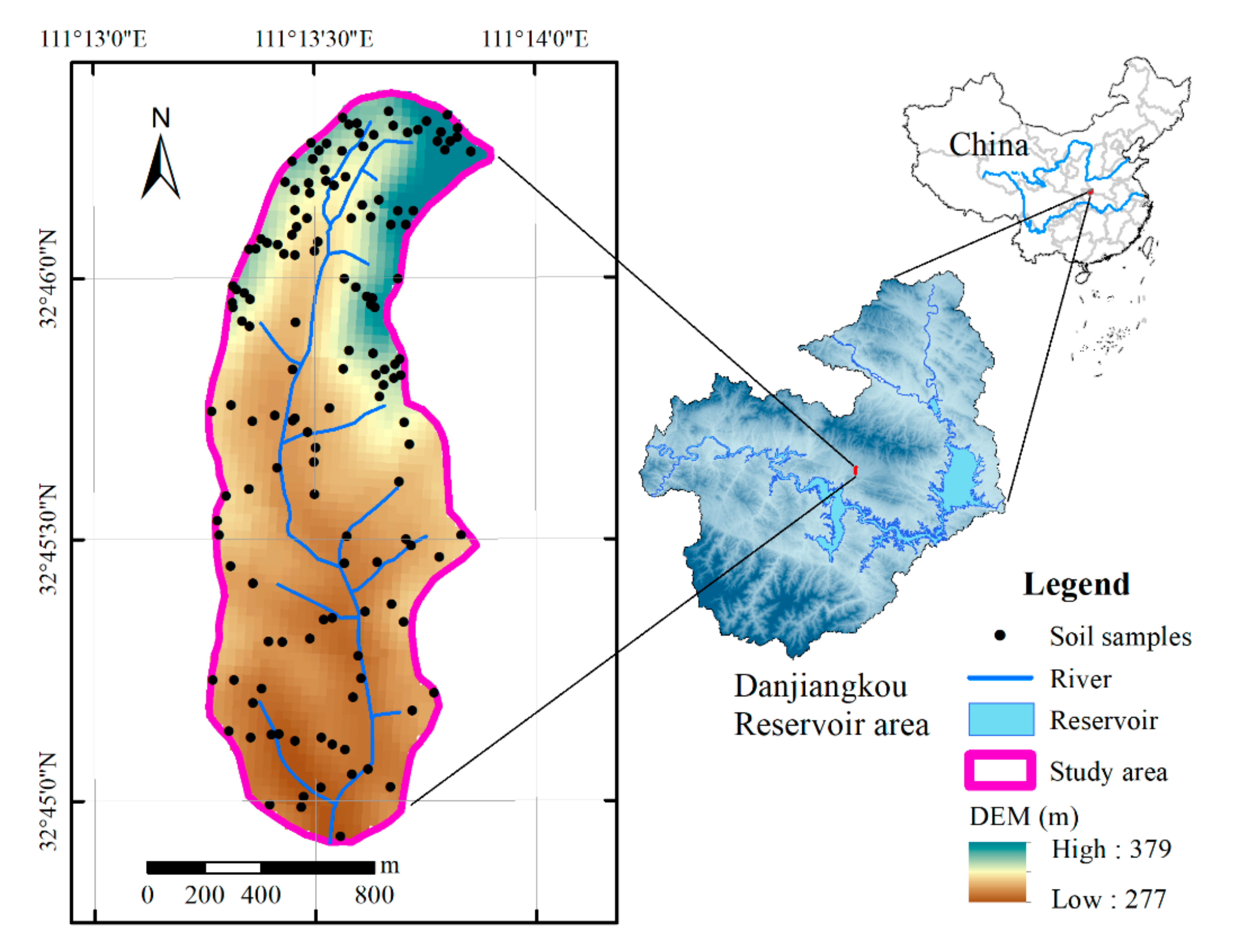
Figure 1. Geographical location of the study area and sampling sites.
Remotesensing 12 03103 g001
Figure 2. Boxplots of the K factor under different land-use types. The uppercase letters represent significant differences in K factor between natural land and cultivated land; the lowercase letters represent significant differences in K factor among woodland, shrubland, terrace, and slope farmland. n, number of samples; CV, coefficient of variation; NL, natural land; CL, cultivated land; W, woodland; S, shrubland; T, terrace; SF, slope farmland.
Remotesensing 12 03103 g002
Figure 3. Soil reflectance spectra in different land-use types (a); and the Pearson correlation coefficients (r) between K factor and Vis–NIR spectra (b).
Remotesensing 12 03103 g003
Figure 4. Variable importance projection (VIP) scores (blue line) and b-coefficients (black line) associated with the cross-validation of PLSR model for K factor prediction using Vis–NIR spectroscopy. The threshold for VIP was set to 1 (blue horizontal dashed line), and the threshold for the b-coefficients was based on their standard deviation (σ = 0.0057; black horizontal dashed lines).
Remotesensing 12 03103 g004
Figure 5. Transferability of PLSR models for the K factor estimation in different sample datasets as assessed by: (a) determination coefficient for validation (R2P); and (b) RPDP. TS, total sample; NL, natural land; W, woodland; S, shrubland; CL, cultivated land; T, terrace; SF, slope farmland.
Remotesensing 12 03103 g005
Figure 6. Pearson’s correlation coefficients between topographic variables and soil K: (a) elevation (m); (b) slope (degree); (c) slope position (percent); (d) watershed location (percent); (e) topographic position index; (f) topographic wetness index; (g) slope height (m); and (h) normalized height.
Remotesensing 12 03103 g006
Figure 7. Scatter plots of referenced versus predicted K factors (Mg h Mj−1 mm−1) for the initial (ac) and improved (df) PLSR models calibrated from spectra and related topographic variables: (a,d) total samples; (b,e) natural land datasets; and (c,f) cultivated land datasets (the red line represents the regression line between the predicted and reference values, and the black line corresponds to the 1:1 line).
Remotesensing 12 03103 g007
Table 1. Descriptive statistics of soil properties in the study area (n = 138).
Soil PropertiesRangeMeanMedianStdCVSkewnessKurtosis
Clay (%)4.33–34.6414.4814.604.8433.450.524.48
Slit (%)22.35–70.2643.8244.357.4216.93−0.143.81
Sand (%)15.02–73.3241.7040.7910.6225.460.543.46
pH5.37–8.648.098.270.597.27−2.6910.30
Bulk density (g cm−3)0.92–1.611.301.310.1612.02−0.102.23
SOC (g kg−1)2.49–18.657.616.253.7849.670.963.29
K (Mg h Mj−1 mm−1)0.027–0.0570.0420.0420.00613.10−0.563.48
SOC, soil organic carbon; K, soil erodibility factor; Std, standard deviation; CV, coefficient of variation.
Table 2. Results of the descriptive statistical analysis of the topographic variables in the study area.
VariableMinimumMaximumMeanStdCV (%)
Slope position (%)1.539953.7532.4760.4
Watershed location (%)0.6496.5459.6628.2447.34
Elevation (m)277.00379.00313.9823.237.40
Slope (°)0.0027.005.455.52101.37
Slope height (m)2.9938.1410.838.7480.69
Normalized height0.110.930.500.2549.50
Topographic position index-4.117.900.602.64438.96
Topographic wetness index4.8617.157.572.4031.71
Std, standard deviation; CV, coefficient of variation.
Table 3. Calibration and cross-validation results of PLSR models for predicting soil K factor for different land-use types.
DatasetnCalibrationCross-Validation
LVsR2CRMSEC
(Mg h Mj−1 mm−1)
R2CVRMSECV
(Mg h Mj−1 mm−1)
RPDCV
Total Samples13890.790.00250.710.00301.84
Natural land6360.860.00240.790.00292.20
Woodland4360.860.00220.740.00301.99
Shrubland2090.970.00090.620.00321.56
Cultivated land7570.530.00240.300.00301.18
Terrace64150.960.00070.460.00281.32
Slope farmland1160.930.00050.190.00200.96
n, number of samples; LVS, number of latent variables; R2C and R2CV, coefficient of determination of calibration and cross-validation models; RMSEC and RMSECV, root mean square error of calibration and cross-validation models; and RPDCV, residual prediction deviation of cross-validation models.