Optical Remote Sensing Image Registration Using Spatial-Consistency and Average Regional Information Divergence Minimization via Quantum-Behaved Particle Swarm Optimization

Abstract

Due to invariance to significant intensity differences, similarity metrics have been widely used as criteria for an area-based method for registering optical remote sensing image. However, for images with large scale and rotation difference, the robustness of similarity metrics can greatly determine the registration accuracy. In addition, area-based methods usually require appropriately selected initial values for registration parameters. This paper presents a registration approach using spatial consistency (SC) and average regional information divergence (ARID), called spatial-consistency and average regional information divergence minimization via quantum-behaved particle swarm optimization (SC-ARID-QPSO) for optical remote sensing images registration. Its key idea minimizes ARID with SC to select an ARID-minimized spatial consistent feature point set. Then, the selected consistent feature set is tuned randomly to generate a set of M registration parameters, which provide initial particle warms to implement QPSO to obtain final optimal registration parameters. The proposed ARID is used as a criterion for the selection of consistent feature set, the generation of initial parameter sets, and fitness functions used by QPSO. The iterative process of QPSO is terminated based on a custom-designed automatic stopping rule. To evaluate the performance of SC-ARID-QPSO, both simulated and real images are used for experiments for validation. In addition, two data sets are particularly designed to conduct a comparative study and analysis with existing state-of-the-art methods. The experimental results demonstrate that SC-ARID-QPSO produces better registration accuracy and robustness than compared methods.

1. Introduction

Image registration is a fundamental process of aligning two or more images (referred to as the reference image and the sensed image respectively) of the same scene taken at different times, from different viewpoints, and/or by different sensors and transforms them into unified coordinate system [1]. It is a crucial pre-process in many optical remote sensing image applications in which the required information must be obtained by integrating various data sources. Therefore, an accurate, effective, and robust image registration is a key success for follow-up data processing.

Over the past decades, many methods for optical remote sensing image registration have been developed and reported in the literature, and can be generally categorized into feature-based methods (FBMs) [2,3,4,5,6,7,8,9,10,11,12,13,14,15,16,17,18,19,20,21,22,23], area-based methods (ABMs) [24,25,26,27,28,29,30,31,32,33,34,35], and joint area-feature based methods (AFBMs) [36,37,38,39,40,41], each of which each of which has been reviewed in great detail in [41].

Generally speaking, ABMs usually obtain higher registration accuracy than FBMs. On the contrary, FBMs are more suitable for registering image pairs with scale difference. ABMs require prior knowledge of initial parameters for multiresolution image registration. By taking advantage of the robustness of features to scale variants and the high precision of similarity metrics, AFBMs integrates information obtained from local features and similarity metrics to effectively register images with large geometric and grayscale differences. Specifically, there are three strategies which integrate ABMS and FBMS into a joint AFBM. As for the first strategy, FBMs are first used to calculate initial parameters for the follow-up ABMs to refine alignment accuracy. For example, [36] implemented a scale-invariant feature transform (SIFT)-based method to calculate pre-registration parameters, which were refined based on maximum mutual information (MI) found by a post-registration process by maximizing MI. In [37], MI was replaced by regional mutual information (RMI). As for the second strategy FBMs were also implemented to performed pre-registration as the first one step with the difference that local features were tuned by similarity metrics (SMs) in the post-registration. There are several works are reported along this line [38]. Proposed a pre-registration method by the scale restricted SIFT [23] and then followed by tuning Harris’ corner in conjunction with a local self-similarity descriptor by normalized correlation coefficient to yield more accurate positions of feature pairs. As for the third strategy, selecting a consistent feature set based on spatial constraint and intensity information is implemented simultaneously. One interesting approach is the iterative SIFT (ISIFT) proposed in [41], which developed an iterative image registration approach that can be used to select consistent feature point sets obtained by maximizing similarity with spatial constraint to update registration parameters in an iterative manner.

Different from ISIFT in [41], this paper follows an idea of using intensity similarity/discrepancy metrics (SM/DM) to fine tune registration parameters by using an optimization process of registration parameters, which maximize/minimize the objective function derived from SM/DM using the SM/DM and SC-based initialized parameters. To do so, it requires an optimization procedure to find the best transformation parameters. Basically, such parameter optimization methods can be divided into two categories, gradient-based optimization methods (GBMs) [29,30,31,32,36] and evolutionary methods (EVMs) [24,37,38,42,43,44,45,46]. For GBMs, [31] proposed a stochastic gradient, called a simultaneous perturbation stochastic approximation search strategy, to accelerate the process of maximizing MI, which is a multiresolution framework based on wavelet-like pyramid decomposition. Another method [32] is developed a stochastic gradient approach to solve the parameters on a proposed frequency domain surface of MI. As a modified method, [36] proposed a Marquardt–Levenberg search strategy using multiresolution to maximize MI in the post-registration. These methods basically use the traditional MI to optimize registration parameters. For many modified versions of MI, EVMs are developed to avoid calculating the gradient similarity between registration parameters. For example, simulated annealing [44], ant colony optimization [24,45], particle swarm optimization (PSO) [42,43,44,46,47] and quantum-behaved PSO (QPSO) algorithm [38,47,48], and chaotic quantum particle swarm optimization implemented in [37], have used modified-MI for finding optimal registration parameters. Among them, QPSO is of particular interest by introducing quantum theory into PSO, which theoretically guaranteed that the optimal solution can be found in search space [47,48].

By taking advantage of the robustness of features to scale variance and the high precision of similarity metrics to intensity difference, a novel AFBM is developed in this paper. Inspired by the concept of spectral information divergence (SID) [49], which measures the discrepancy of probabilistic behaviors between the spectral signatures, this paper proposes an average regional information divergence (ARID) as DM. The developed ARID is quite different from the above-mentioned MI-based methods or modified versions in the sense that it not only makes use of statistics derived from intensity correlation and spatial consistency information but also avoids calculating the joint probability distribution. Additionally, unlike the above-mentioned AFBMs, this paper further develops a two-component cascaded registration method, to be called spatial-consistency and average regional information divergence minimization via QPSO (SC-ARID-QPSO) as shown in Figure 1 for optical remote sensing images registration. It combines SC and intensity discrepancy in different manners. Specifically, it can be implemented by two components in cascade with a SM/DM-based consistent feature set selection implemented in the first component, Component I, followed by the second component, Component II, which iteratively optimizes registration parameters by maximizing/minimizing SM/DM with the spatial constraint via optimization algorithm. The key idea of SC-ARID-QPSO is to jointly use ARID with spatial consistency throughout these two components.

The remainder of this paper is organized as follows. The proposed regional information divergence (RID) is described in Section 2. SC-RID-QPSO is described in Section 3. Novelties of SC-ARID-QPSO is given in Section 4. The experimental setting is detailed in Section 5 followed by a comparative study of extensive experiments along with their results in Section 6. The discussion of experimental results, phenomenon analysis, and future work are presented in Section 7. Finally, a brief conclusion and contributions are summarized in Section 8.

2. Average Regional Information Divergence

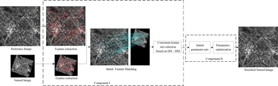
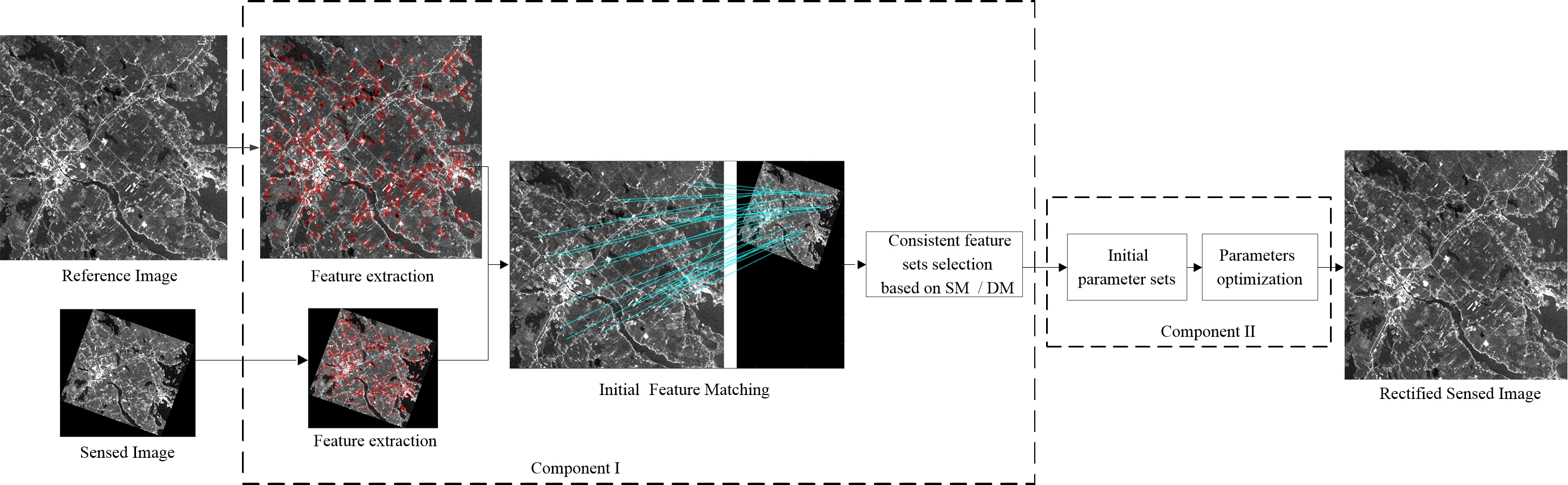
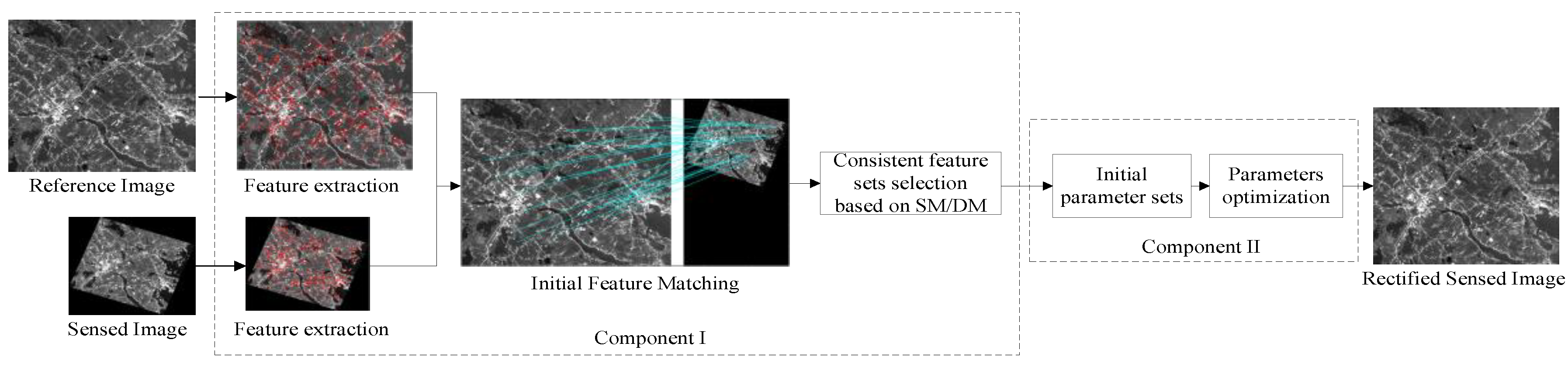
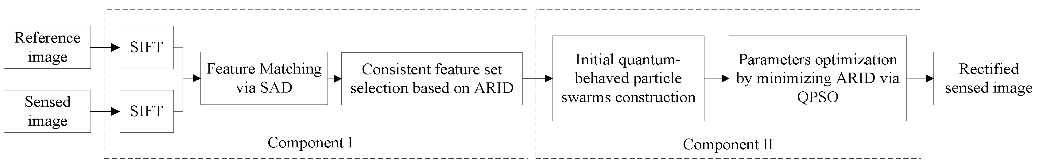
Inspired from the concept of spectral information divergence (SID) [39], which measures the discrepancy of probabilistic behaviors between the spectral signatures, we drive a discrepancy metric based on region information divergence to capture the intensity correlation between overlapping region of reference image R and rectified sensed image S_rec. For each pixel $P_i^R$ and $P_i^{S_{\mathbf{rec}}}$ in overlapping regions, the intensity vectors of local neighborhood region with radius $r$ are $v_i^R={(v_{i_1},\dots ,v_{i_L})}^T$ and $w_i^{S_{\mathbf{rec}}}={(w_{i_1},\dots ,w_{i_L})}^T$, $L={(2r+1)}^2$. Assume that $p_i^R={(p_{i_1},\dots ,p_{i_L})}^T$ and $q_i^{S_{\mathbf{rec}}}={(q_{i_1},\dots ,q_{i_L})}^T$ are probability vector corresponding $v_i^R={(v_{i_1},\dots ,v_{i_L})}^T$ and $w_i^{S_{\mathbf{rec}}}={(w_{i_1},\dots ,w_{i_L})}^T$ where $p_{i_l}=v_{i_l}/{\displaystyle {\sum }_{l=1}^L{v}_{i_l}}$ and $q_{i_l}=w_{i_l}/{\displaystyle {\sum }_{l=1}^L{w}_{i_l}}$. From information theory and spectral information divergence (SID) [39], we can define the region information divergence (RID) between $v_i^R$ and $w_i^{S_{\mathbf{rec}}}$ similar to SID by

$$\begin{array}{rr}\mathrm{RID}(v_i^R,w_i^{S_{\mathbf{rec}}})=& D(v_i^R||w_i^{S_{\mathbf{rec}}})+D(w_i^{S_{\mathbf{rec}}}||v_i^R)\hfill \\ =& {\displaystyle {\sum }_{l=1}^L{p}_{i_l}{D}_l(v_i^R||w_i^{S_{\mathbf{rec}}})}+{\displaystyle {\sum }_{l=1}^L{q}_{i_l}{D}_l(w_i^{S_{\mathbf{rec}}}||v_i^R)}\hfill \\ =& {\displaystyle {\sum }_{l=1}^L{p}_{i_l}\log \left(\frac{p_{i_l}}{q_{i_l}}\right)}+{\displaystyle {\sum }_{l=1}^L{q}_{i_l}\log \left(\frac{q_{i_l}}{p_{i_l}}\right)}\hfill \end{array}$$

(1)

According to (1) an overlapped region (OR) in the reference image and rectified images can be further defined by taking the average of $\mathrm{RID}(v_i^R,w_i^{S_{\mathrm{rec}}})$ over $(v_i^R,w_i^{S_{\mathrm{rec}}})\in \mathrm{OR}$ as average region information divergence (ARID)

$${\mathrm{ARID}}^{\mathrm{OR}}=\frac{1}{\left|\mathrm{OR}\right|}{\displaystyle {\sum }_{(v_i^R,w_i^{S_{\mathrm{rec}}})\in \mathrm{OR}}\mathrm{RID}(v_i^R,w_i^{S_{\mathrm{rec}}})},$$

(2)

where $\left|\mathrm{OR}\right|$ is the total number of pixels in OR. Using (2) ARID can be used to measure the region discrepancy metric between reference image and rectified sensed image. As a result, the smaller is the value of ARID, the higher is the accuracy of the registration parameters.

3. SC-ARID-QPSO

The idea of SC-ARID-QPSO was briefly introduced in Section 1. The entire process of SC-ARID-QPSO is depicted in Figure 2 which implements two components in a cascade manner where the first component, Component I, is to produce a spatial consistent feature set to be used for generating initial particle swarms for QPSO; and the second component, Component II, is to implement QPSO for minimizing ARID using ARID-constrained initialized parameter set. In Component I, local features are extracted from the reference image and sensed image by SIFT, respectively. It is further followed by a spectral angular distance (SAD)-based feature matching to obtain initial matching feature set. Then, the consistent feature sets are obtained by minimizing ARID with spatial constraint. In Component II, the M initial parameter sets are calculated by fine-tuned consistent feature sets, which are generated by randomly tuning the selected consistent feature sets through a number of times constrained by ARID values where M is empirically determined. The obtained initial parameter sets are further used to produce initial particle swarms for QPSO, which minimizes ARID to find final optimal registration parameters. Figure 2 provides the step-by-step details of implementing each of the above-mentioned two-component cascaded registration method, which is clearly different from ISIFT in [41].

3.1. Component I: Consistent Feature Set Selection

3.1.1. Feature Extraction and Matching

The first part of the Component I is to find initial matching feature points by SIFT [2], which consists of feature extraction and description. Then, the ratio of the nearest neighbor to the second-nearest neighbor [26] based on the SAD [49] is calculated to be used for the selection of the initial matching feature set.

SIFT selects the local maxima and minima of D(x) in scale space as candidate feature points. In order to obtain more accurate position, detailed fit to the nearby data samples is performed in scales-spatial spaces. Unstable feature points are rejected based on contrast values and principal curvature ratios of features. Then, a dominant orientation is assigned to each feature point based on gradient orientations of features within a local region to achieve rotation invariance. Finally, a 128-D descriptor based gradient histogram is constructed in a local region of each feature point. The initial feature matching is performed by using SAD [50] to measure the discrepancy between two descriptors defined by

$$\theta ={\cos }^{-1}\left(\frac{a_i^T{b}_i}{\Vert a_i\Vert \Vert b_i\Vert }\right),$$

(3)

where $a_i$ is the ith feature descriptor vector in the sensed image, $b_i$ is the ith feature descriptor vector in the reference image, and ${\theta }_{ratio}$ is the angle between the two vectors. The ratio of the first minimum angle to the second-minimum angle [31] denoted by ${\theta }_{ratio}$ is used. If the initial match features with angle distance ratios are smaller than a threshold ${\theta }_{ratio}$, they are remained.

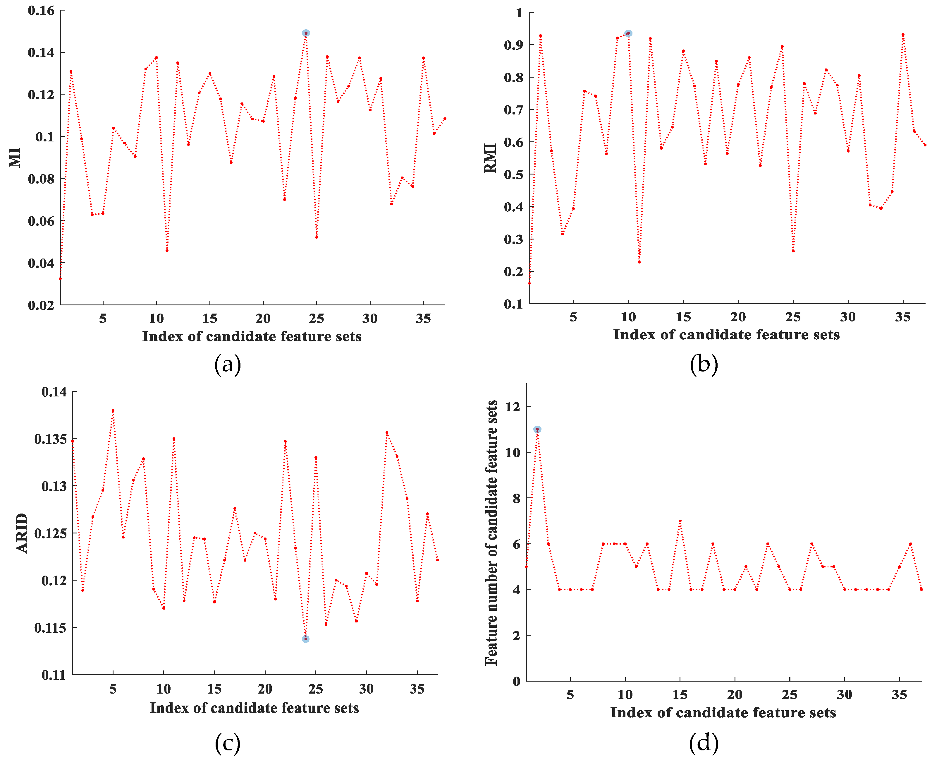
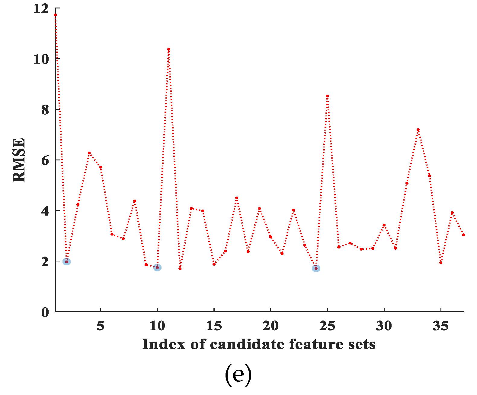
3.1.2. Consistent Feature Set Selection Based on ARID

On the basis of the initial feature matching, an effective outlier elimination can be further used to improve the precision of reserved feature pairs. A similar idea to using the ARID-based method to select a consistent feature set was also proposed in [41]. The details of ARID-based SC feature set selection can be described by the following two steps.

• Implement SIFT and random sample consensus on reference image $R$ and sensed image $S$ to obtain initial consistent feature point sets $S_{\mathrm{feature}}^{(0)}={\left\{{\mathrm{FS}}_j^{(0)}\right\}}_{j=1}^{M_0}$ where ${\mathrm{FS}}_j^{(0)}$ is the jth initial consistent feature point set and M₀ is the number of initial consistent feature point sets.
• Adopt $S_{\mathrm{feature}}^{(0)}={\left\{{\mathrm{FS}}_j^{(0)}\right\}}_{j=1}^{M_0}$ to calculate registration parameters set $S_{\mathrm{parameter}}^{(0)}={\left\{{\mathrm{Pa}}_j^{(0)}\right\}}_{j=1}^{M_0}$ where ${\mathrm{Pa}}_j^{(0)}$ is the jth initial registration parameter and discrepancy values DVs set $V_{\mathrm{ARID}}^{(0)}={\left\{{\mathrm{ARID}}_{{\mathrm{FS}}_j}^{(0)}\right\}}_{j=1}^{M_0}$ for image $R$ and rectified sensed image ${\left\{S_{\mathrm{rect}}^{(0)}\right\}}_{j=1}^{M_0}$ based on $S_{\mathrm{feature}}^{(0)}$. The initial consistent feature point set ${\mathrm{FS}}_{j*}$ is selected based on minimum ARID, denoted by ${\mathrm{ARID}}_{\min }^{(0)}$, where $j^{*}=\arg \left\{{\min }_{{\mathrm{FS}}_j\in S_{\mathrm{feature}}}{\mathrm{ARID}}_{{\mathrm{FS}}_j}\right\}$.

3.2. Component II: Fine Registration by Minimizing Average Regional Information Divergence (ARID) via QPSO

After the consistent feature set being selected, the registration parameters are optimized by minimizing ARID via QPSO. In order to implement QPSO, initial particle swarms must be specified first.

3.2.1. Initial Parameters of QPSO Generated by the Consistent Feature Set Obtained in Component I

• Find the coordinate of feature points in ${\mathrm{FS}}_{j*}$ by randomly tuning parameter b to generate tuned feature point sets $S_{\mathrm{feature}}^{\mathrm{tuned}}={\left\{{\mathrm{FS}}_{j_p^{*}}\right\}}_{p=1}^{\tilde{M}}$.
• Adopt ${\left\{{\mathrm{FS}}_{j_p^{*}}\right\}}_{p=1}^{\tilde{M}}$ to calculate a registration parameters set $S_{\mathrm{parameter}}^{(0)}={\left\{{\mathrm{Pa}}_{j_p^{*}}^{(0)}\right\}}_{p=1}^{\tilde{M}}$ and corresponding DVs set $V_{{\mathrm{ARID}}_{j_p^{*}}}^{(0)}={\left\{{\mathrm{ARID}}_{{\mathrm{FS}}_{j_p^{*}}}^{(0)}\right\}}_{p=1}^{\tilde{M}}$. The first M particles, which have smaller DVs than ${\mathrm{ARID}}_{\min }^{(0)}$, are used as initial particle swarms ${\left\{{\mathrm{P}}_m^{(0)}\right\}}_{m=1}^M$. If there are not M particle satisfying the DVs are less than ${\mathrm{ARID}}_{\min }^{(0)}$, the number of tuned feature set $\tilde{M}$ should be increased. The initial particle swarms are also used as initial local optimum particles ${\left\{{\mathrm{P}}_l^{(0)}\right\}}_{l=1}^M={\left\{{\mathrm{P}}_m^{(0)}\right\}}_{m=1}^M$ and the corresponding ARID is denoted by ${\left\{{\mathrm{ARID}}_p^{(0)}\right\}}_{p=1}^M$.
• Select the particle ${\mathrm{P}}_{l^{*}}^{(0)}$ corresponding minimum ARID among ${\left\{{\mathrm{ARID}}_m^{(0)}\right\}}_{m=1}^M$, denoted by ${\mathrm{ARID}}_{\min }$, as the global optimum particle ${\mathrm{P}}_g^{(0)}$.

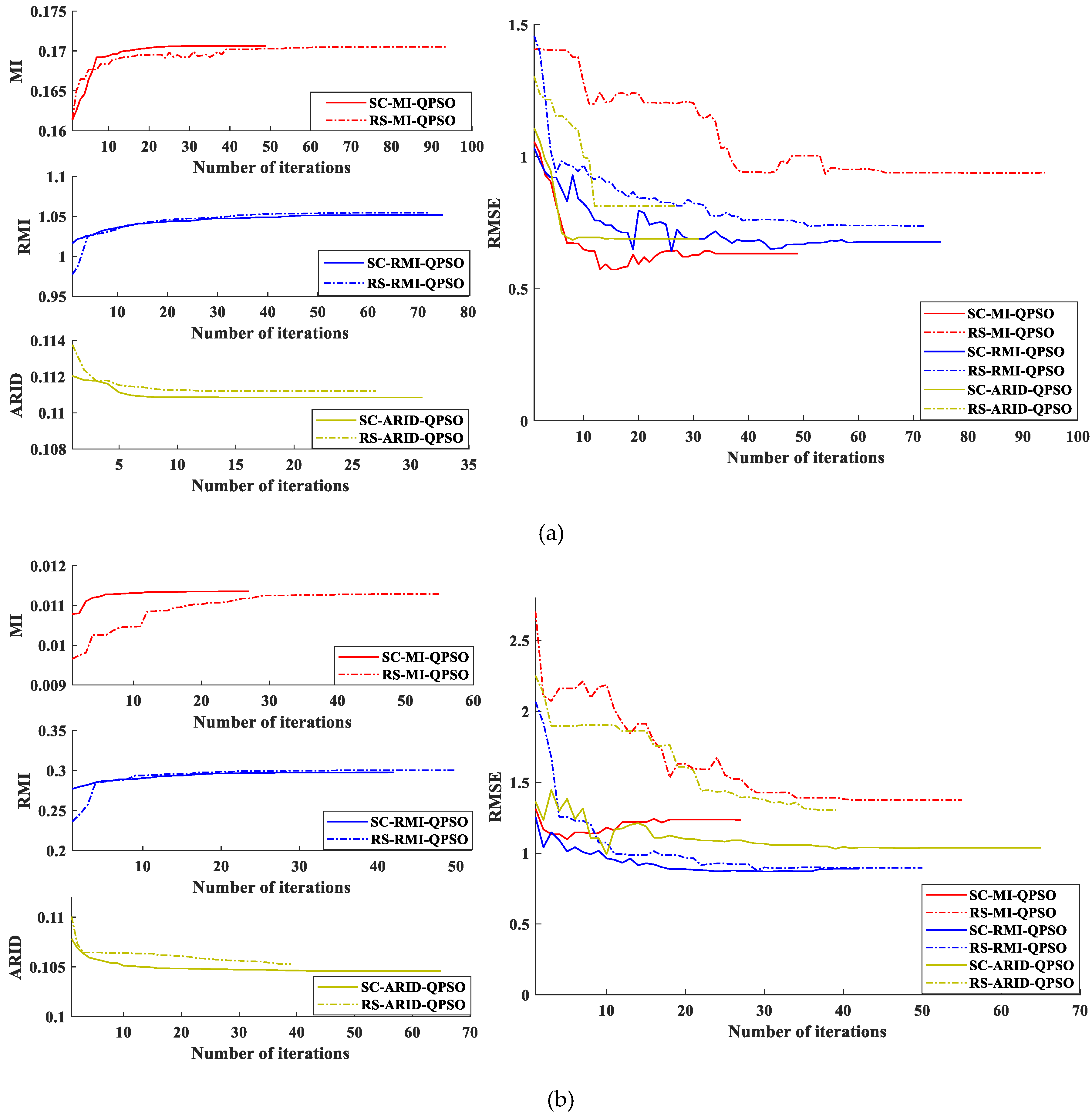
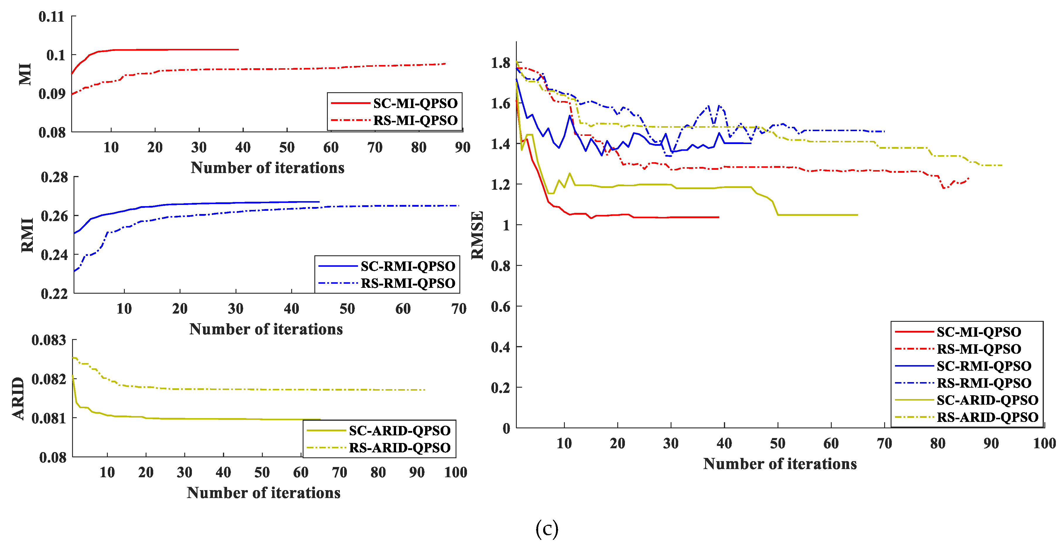
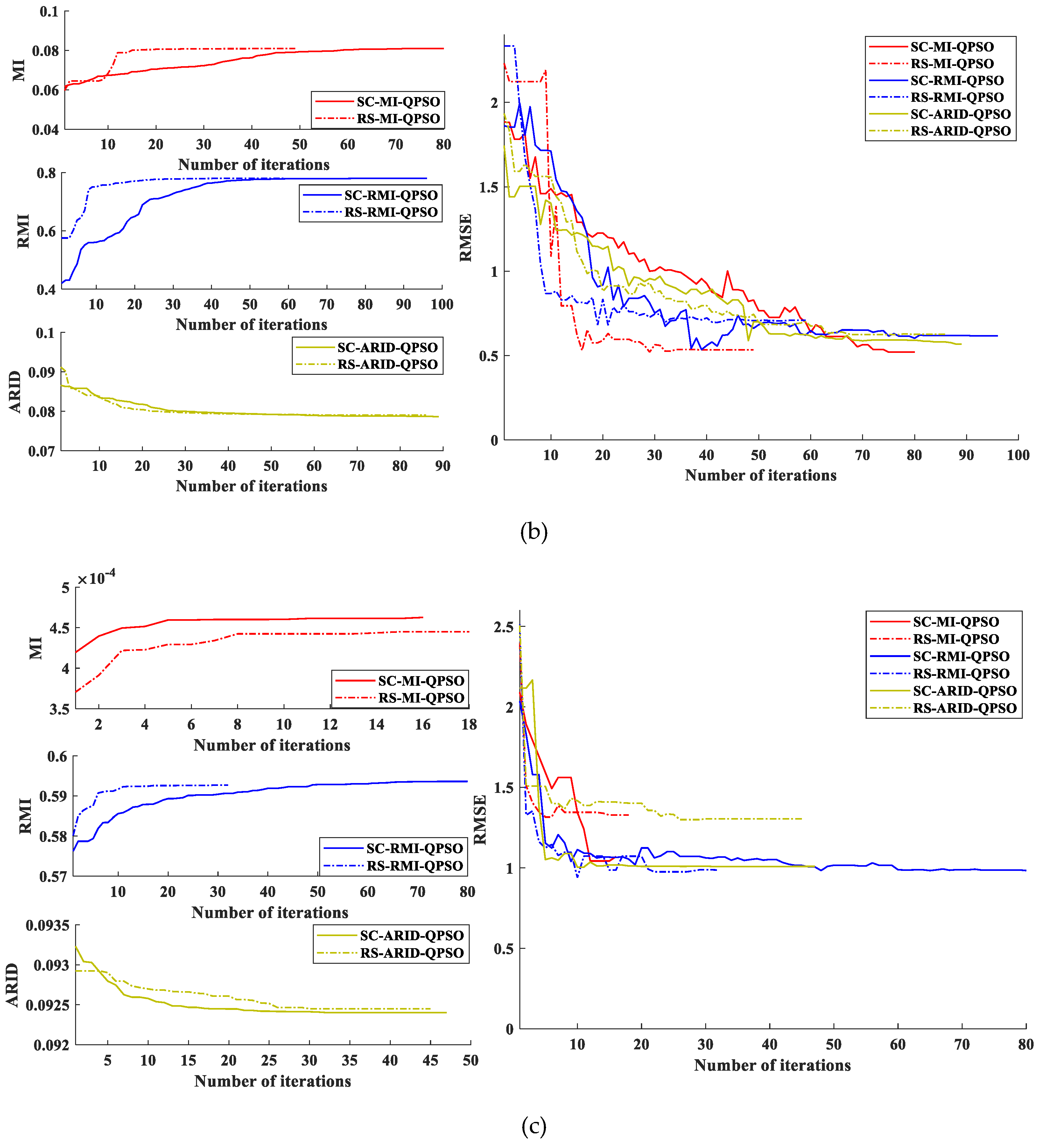
3.2.2. Parameters Optimized by Minimizing ARID via QPSO

In QPSO, each particle only has its position information $X_m^{(k)}=(X_{m1}^{(k)},X_{m2}^{(k)},\dots ,X_{mD}^{(k)})$ in a D-dimensional space and represents a solution of the problem, specified by a set of registration parameters, where k is the current number of iteration and m is the mth particle in M particle swarms.

In the very beginning, the local optimal position ${\left\{{\mathrm{P}}_l^{(0)}\right\}}_{l=1}^M$ and ${\mathrm{P}}_g^{(0)}$ are provided by initialization. The particle positions are updated by the evolution equation, which is given by

$$m_{\mathrm{best}}^{(k)}={\displaystyle {\sum }_{l=1}^M{P}_l^{(k)}}/M,$$

(4)

$$p_{md}^{(k)}={\varphi }_d^{(k)}·P_{ld}^{(k)}+[1-{\varphi }_d^{(k)}]·P_{gd}^{(k)},$$

(5)

$$X_{md}^{(k+1)}=p_{md}^{(k)}\pm \beta \left|m_{\mathrm{best}}^{(k)}-X_{md}^{(k)}\right|·\ln \left(\frac{1}{u_{md}^{(k)}}\right),$$

(6)

where $u_{md}^{(k)}$ and ${\varphi }_d^{(k)}$ are random numbers distributed uniformly in interval (0,1). $\beta$ is an expansion-contraction factor, which is defined as follows:

$$\beta =\left({\alpha }_0-{\alpha }_1\right)\times (N_{\max }-N_{current})/N_{\max }+{\alpha }_0$$

(7)

where $N_{\max }$ is the maximum iteration number and $N_{current}$ is the current iteration number. ${\alpha }_0$ and ${\alpha }_1$ are initial and final values of the control parameter respectively and ${\alpha }_0>{\alpha }_1$. An automatical stopping rule is determined by two ASID values corresponding global particle warm ${\mathrm{P}}_g^{(k)}$ and ${\mathrm{P}}_g^{(k-1)}$. Let n be the number of times that $\left|{\mathrm{ARID}}_{\min }^{(k-1)}-{\mathrm{ARID}}_{\min }^{(k)}\right|\le \tau$ is satisfied. In this case, n = n + 1, else n = 0. If the number of iterations reaches $N_{\max }$ or n reaches n_τ, the iteration is terminated. The detailed description of SC-ARID-QPSO is provided in the following.

Algorithm1. SC-ARID-QPSO

Input: reference image ${\mathbf{R}}^{(0)}$, sensed image ${\mathbf{S}}^{(0)}$, the number of iterations, k, the number of no updating, n, maximum iterative number $N_{\max }$ = 100, threshold τ = 10−4 and nτ = 15, coordinate tuning parameter b, particle population M = 20, Particle dimension D = 6 (for affine model) or 8 (for projective model) control parameters α0 and α1, initial particle swarm $X_i$ (i = 1, 2, …, M), tuning range $b\in \left(-0.5,0.5\right)$.

Output: Final registration parameters

1. Initialize: $\mathbf{R}={\mathbf{R}}^{(0)}$, $\mathbf{S}={\mathbf{S}}^{(0)}$ and k = 0, n = 0.

2. Initialization of initial local optimum particle ${\left\{{\mathrm{P}}_l^{(0)}\right\}}_{l=1}^M$ and global optimum particle ${\mathrm{P}}_g^{(0)}$.

3. Implement QPSO to optimize registration parameters:

While k < $N_{\max }$ do;

Calculate β using Equation (7) and $mbes{t}^{(k-1)}$ using Equation (4).

For m = 1:M do

For d = 1:D do

Calculate $p_{md}^{(k-1)}$ and $X_{md}^{(k)}$ using Equation (5) and Equation (6).

End for

Calculate ${\mathrm{ARID}}_m^{(k)}$ based on $X_{md}^{(k)}$ using (2) and (3).

If ${\mathrm{ARID}}_m^{(k-1)}\ge {\mathrm{ARID}}_m^{(k)}$ then ${\mathrm{ARID}}_{\mathrm{m}}={\mathrm{ARID}}_{\mathrm{m}}^{(k)}$, ${\left\{{\mathrm{P}}_l^{(k)}\right\}}_{l=m}={\left\{X_{md}^{(k)}\right\}}_{d=1}^D$,  End if

End for

${\mathrm{ARID}}_{\min }^{(k)}=\min \left({\left\{{\mathrm{ARID}}_m^{(k)}\right\}}_{m=1}^M\right)$

If ${\mathrm{ARID}}_{\min }^{(k-1)}\ge {\mathrm{ARID}}_{\min }^{(k)}$ then ${\mathrm{ARID}}_{\min }={\mathrm{ARID}}_{\min }^{(k)}$, ${\mathrm{P}}_g^{(k)}=\arg \underset{P_l^{(k)}}{\min }{\mathrm{ARID}}_m^{(k)}$,  End if

If $\left|{\mathrm{ARID}}_{\min }^{(k-1)}-{\mathrm{ARID}}_{\min }^{(k)}\right|\le \tau$ then n = n + 1

If $n>n_{\tau }$ then Break, End if

End if

End while

4. Return ${\mathrm{P}}_g^{(k)}$ as final registration parameters

4. Novelties of SC-ARID-QPSO

There are several novelties derived from SC-ARID-QPSO which can be summarized as follows.

• The first novelty is introduction of ARID, which considers a neighboring region as a random variable. Such ARID is quite different from RMI and RIRMI in the sense that the latter was calculated under the assumption that high-dimensional distribution is approximately normally distributed, while the former defines the desired probability distribution by normalizing its neighborhood region histogram to unity. The discrepancy between the overlapped regions of reference image and rectified sensed image is calculated by averaging the values of RID of all pixels in the overlapped region without a need of calculating their joint probability distribution.
• The Second novelty is to develop a two-component cascaded registration method which optimizes spatial-consistency and ARID registration parameters. In contrast to most AFBMs [36,37] which only uses the pre-registration as initial parameters for the fine registration, SC-ARID-QPSO uses pre-registration based on SC and ARID to initialize the parameters for fine registration. The process of ARID-constrained parameter initialization guarantees the quality of initialized parameter set. In particular, it is quite different from an AFBM developed in [41], called iterative SIFT (ISIFT) which replaces the sensed image via a feedback loop to re-implement registration process. More specifically, ISIFT iteratively feeds a rectified image to replace the current sensed images, while SC-ARID-QPSO iteratively optimizes the registration parameters using an ARID-based objective function with the ARID-constrained initialized parameter set from the same set of the reference and sensed images.
• The last and most important novelty is fundamental different concepts used to derive ISIFT and SC-ARID-QPSO. Despite the fact that both ISIFT and SC-ARID-QPSO use an iterative process, the ISIFT feeds back rectified images to update the input sensed images as opposed to SC-ARID-QPSO, which uses QPSO iteratively to optimize parameter sets. So, ISIFT [41] and SC-ARID-QPSO are designed based on different uses of iterative processes since they both use spatial-consistency and intensity-similarity to perform different tasks. However, it is worth noting that there are several key differences between ISIFT and SC-ARID-QPSO. First of all, SC-ARID-QPSO takes advantage of QPSO to optimize registration parameter by minimizing ARID via optimization algorithm, while ISIFT does not. Second of all, SC-ARID-QPSO develops ARID as a novel discrepancy metric compared to ISIFT which uses traditional similarity metrics. Third of all, although the experimental datasets used in this paper are the same as the datasets in reference [41], their purposes are different. In this paper, the experimental results are used to demonstrate the effectiveness of ARID and the performance of SC-ARID-QPSO as opposed to ISIFT which used the data sets to show effectiveness of consistent feature selection strategy and iterative performance of ISIFT. Specifically, in Component I, the designed experiments are used for validating the accuracy and effectiveness of ARID. In Component II, the designed experiments are used to demonstrate the iterative process of parameter optimization by minimizing ARID via QPSO as well as the effective selection of initialized parameter set. In addition, the comparative experiments further show the superior performance of SC-ARID-QPSO to compared methods.

5. Experimental Setting

In order to validate the performance of SC-ARID-QPSO, two groups of data sets are used for experiments and are acquired from different bands, different resolution, the same/different sensors, and the same/different time. Experimental datasets are diverse, including aerial and satellite images, and has affine or projection distortion, involving scale differences, rotation differences, translation differences, and perspective differences. In addition, because the data contains different sensors at different times, it also has grayscale differences.

The proposed SC-ARID-QPSO was implemented in MATLAB. In order to compare the performance of ARID with other common similarity metrics, such as MI and RMI, we implemented the SC-ARID-QPSO with different metrics to replace ARID. Thus, it yielded two different versions, called spatial consistent (SC) with MI maximization via QPSO (SC-MI-QPSO), and SC with RMI maximization via QPSO (SC-RMI-QPSO). For comparing performance of Component I by SC with SM or RANSAC, different versions, called SC with MI (SC-MI), SC with RMI (SC-RMI), and SC with ARID (SC-ARID) were used. For comparing the results obtained in Component II, different initial consistent feature sets generated in Component I were also derived, which were RANSAC using MI maximization via QPSO, RANSAC with RMI maximization via QPSO, and RANSAC with ARID minimization via QPSO referred to as RS-MI-QPSO, RS-RMI-QPSO and RS-ARID-QPSO, respectively. More specifically, RANSAC and SC with SM, respectively, selected consistent feature point sets to generate initial particle swarm to optimize parameters by maximizing/minimizing SM/DM via QPSO. However, there is a key difference between the two initial particle swarms generated by RANSAC and SC with SM, as described in the introduction. SC with SM/DM selected a consistent feature set with maximum/minimum similarity value (SV)/DV, which has more accurate registration results than RANSAC. Moreover, the SV/DV of each particle in the initial particle swarm can be constrained by SM/DM to make the initial particle swarm better than the consistent feature set.

As demonstrated above, RS-MI-QPSO, RS-RMI-QPSO, RS-ARID-QPSO, SC-MI-QPSO, SC-RMI-QPSO, and SC-ARID-QPSO were used to compare their optimized results with different initial particle swarms and metrics. So, a total of 6 methods were tested for comparison. Specifically, SC-MI, SC-RMI, SC-ARID, and RANSAC were implemented to compare ARID with other different metrics in the Component I. In addition, to further conduct quantitative analysis, the final root mean square errors (RMSEs) of 6 methods with 2 components were calculated, and the visual displays of final fused registered images are also plotted for comparison.

5.1. Data Sets

The first group contains three simulated datasets and three real datasets, both of which can be used to validate the superior performance of spatial consistent feature point set based on RID (SC-ARID) and SC-ARID with parameters optimization via QPSO (SC-ARID-QPSO). The three simulated image pairs consist of two images selected from different bands, one band as the reference image and another band of corresponding multispectral images with a simulated transformation (2.5-times scale and 20° rotational changes by ENVI [51]) as the sensed image. To verify the performance under real scenes, the three real image sets were obtained from different sensors and taken during the same or different years. These image pairs also cover a variety of spatial resolutions from 2 m to 30 m.

The second group contains 80 images, which were randomly selected from two public available data sets respectively [6,52,53]. The first public available dataset contains 107 multispectral and multitemporal remote sensing image pairs with 512 × 512 [6,52], obtained from the United States Geological Survey (USGS) website [54]. The pixel resolution of these images is 1 m. The second public available dataset [54,55] contains 12 classes scene and a total of 1200 images with 256 × 256. The pixel resolution of this public images is 0.3 m. In order to verify the statistical evaluation performance under affine transformation and projective transformation, two data sets were simulated for experiments as follows. Data set A was generated from 40 image sets, which were randomly selected from the first public available data set. For each data set, one band was selected as reference image and another band was applied a known affine transformation (scaling, rotation, and translation) to generate the sensed image. Data set B was generated from 40 image sets, which were randomly selected from the second public available data set. For each data set, one band was selected as reference image and another band was applied to a known projective transformation (scaling, rotation, translation, and perspective) to create the corresponding sensed image. All these data sets with detailed descriptions are made available at http://wiki.umbc.edu/display/rssipl/10.+Download.

5.2. Parameter Setting

In the component I, the ratio parameter ${\theta }_{ratio}$ used for SAD feature matching. As a tradeoff between the number of correct matches and the rate of correct matches, ${\theta }_{ratio}$ was set to 0.7. The maximum number of iterations for RANSAC was set to 100 based on the calculation equation [15] and experience empirically. The local 8-nieghbor pixels are used for calculating RID. In addition, the threshold of the model referred in [2] was set to 0.5. In the component II, the particle population of particle swarm was set to 20. For the stopping rule, the threshold of difference between similarity values $\mathrm{th}={10}^{-4}$. The number of durations $n_{\tau }=15$ that the different between two consecutive discrepancy value is less than a certain threshold value.

5.3. Evaluation Criteria

Root mean square error (RMSE) was used to quantitatively evaluate the registration position accuracy. For an affine transformation and projective transformation, it is defined respectively by

$$RMS{E}_{\mathrm{affine}}=\sqrt{\frac{1}{k}}\cdot {\Vert \left(\begin{array}{c}\begin{array}{ccc}{\widehat{a}}_1-a_1& {\widehat{b}}_1-b_1& {\widehat{c}}_1-c_1\end{array}\\ \begin{array}{ccc}{\widehat{a}}_2-a_2& {\widehat{b}}_2-b_2& {\widehat{c}}_2-c_2\end{array}\end{array}\right)\left(\begin{array}{c}\begin{array}{cccc}{x}_2^1& x_2^2& \dots & x_2^k\end{array}\\ \begin{array}{cccc}{y}_2^1& y_2^2& \dots & y_2^k\end{array}\\ \begin{array}{cccc}1& 1& \dots & 1\end{array}\end{array}\right)\Vert }_2$$

(8)

$$RMS{E}_{\mathrm{perspective}}=\sqrt{\frac{1}{k}}{\Vert \left(\begin{array}{c}\begin{array}{ccc}{\widehat{a}}_1-a_1\hfill & {\widehat{b}}_1-b_1\hfill & {\widehat{c}}_1-c_1\end{array}\\ \begin{array}{ccc}{\widehat{a}}_2-a_2& {\widehat{b}}_2-b_2& {\widehat{c}}_2-c_2\end{array}\\ \begin{array}{lll}{\widehat{a}}_3-a_3\hfill & {\widehat{b}}_3-b_3\hfill & 0\end{array}\end{array}\right)\left(\begin{array}{c}\begin{array}{cccc}{x}_2^1& x_2^2& \dots & x_2^k\end{array}\\ \begin{array}{cccc}{y}_2^1& y_2^2& \dots & y_2^k\end{array}\\ \begin{array}{cccc}1& 1& \dots & 1\end{array}\end{array}\right)\Vert }_2$$

(9)

where $a_1,a_2,b_1,b_2,c_1,c_2$ and $a_1,a_2,a_3,b_1,b_2,b_3,c_1,c_2$ are the real values of the corresponding model parameter, ${\widehat{a}}_1,{\widehat{a}}_2,{\widehat{b}}_1,{\widehat{b}}_2,{\widehat{c}}_1,{\widehat{c}}_2$ and ${\widehat{a}}_1,{\widehat{a}}_2,{\widehat{a}}_3,{\widehat{b}}_1,{\widehat{b}}_2,{\widehat{b}}_3,{\widehat{c}}_1,{\widehat{c}}_2$ are the estimated values of the corresponding model parameters. As for the ground truth (simulated images) or the reliable reference geometric transformation parameters, they were calculated by manual registration using ENVI.

In addition, the checkboard mosaic images [40] for group 1 are provided for performance evaluation and visual inspection of registration results respectively.

6. Experimental Results

Based on the above demonstration of experimental design, the experimental results of the two groups of data sets are presented in this section, which contain simulated datasets experiments, real datasets experiments, and comparative analysis on registration performance with other methods.

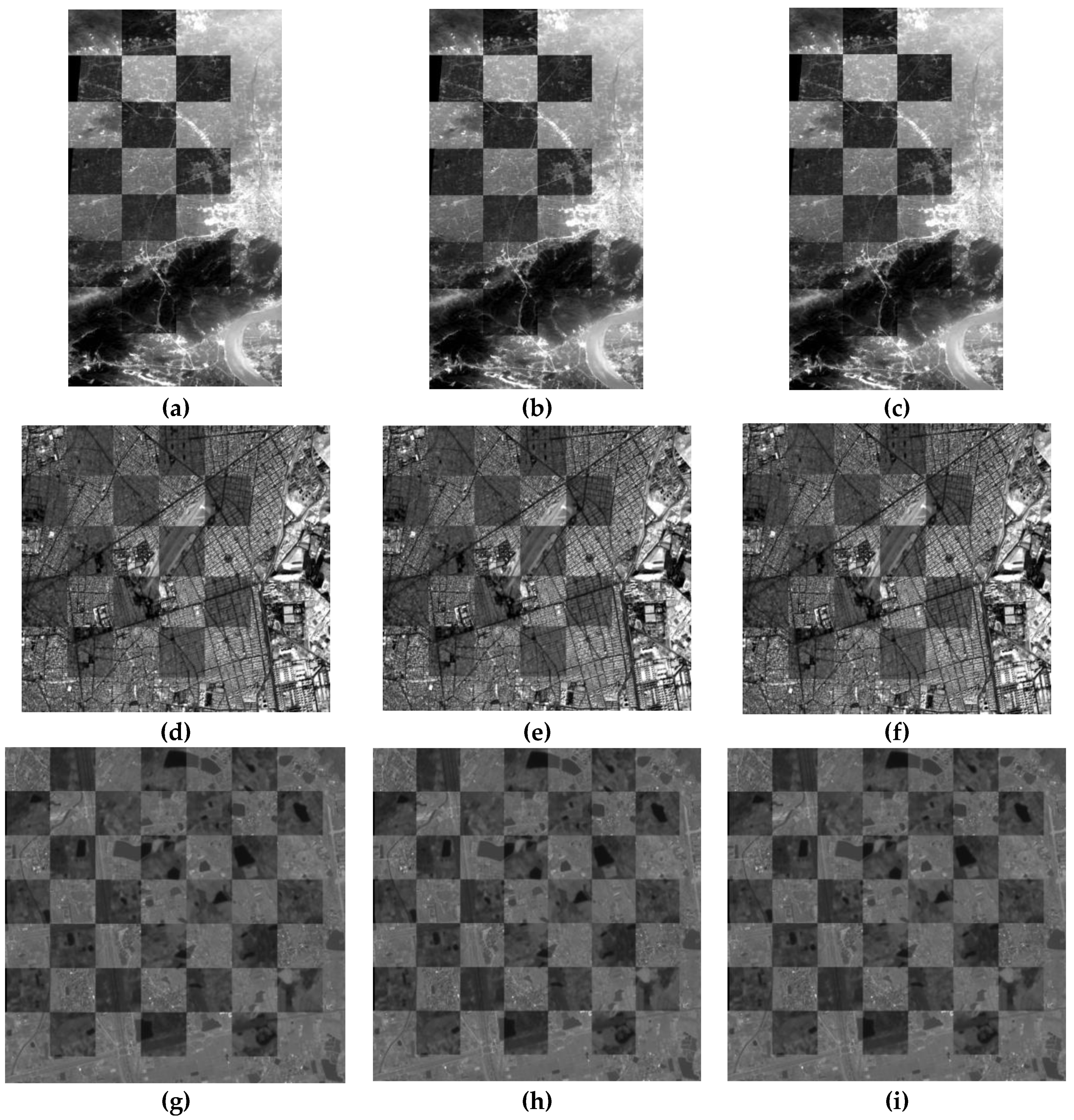
6.1. Simulated Datasets Experiments

Figure 3 shows the SV/DV calculated by MI, RMI, ARID, and inner number of feature sets, respectively, along with the index of feature sets, and RMSEs in each feature set for simulated dataset 1 in Component I. In all figures of Figure 3, the horizontal axes are the index of feature sets, and the vertical axes in Figure 3a–c are SVs/DVs produced by MI, RMI, and ARID, while the vertical axis in Figure 3d is the feature number of each candidate feature set. Figure 3e shows the RMSE versus the index of feature sets where RMSE was calculated by each feature set. The number of feature pairs in each feature set larger than three for affine transformation was retained while the total number of feature sets was set to 100. Thus, the resulting number of each candidate set varies with different images as demonstrated in the experiments conducted in Section 6.

In Figure 3, the selected consistent feature sets by SC-MI, SC-RMI, SC-ARID, and RANSAC and their corresponding RMSE are highlighted by large solid circles. The RMSE calculated by consistent feature set selected by ARID were relatively smaller than or equal to the RMSE calculated by RANSAC. In order to demonstrate the effectiveness of ARID, Figure 3 shows the intuitively selection process in Component I for simulated image 1, and the corresponding RMSE is given in the Component I of

Table 1. Comparison of the final RMSEs for simulated image pairs.

Data Sets	Component I				Component II
	RANSAC	SC-MI	SC-RMI	SC-ARID	RS-MI-QPSO	RS-RMI-QPSO	RS-ARID-QPSO	SC-MI-QPSO	SC-RMI-QPSO	SC-ARID-QPSO
1	1.9764	1.7120	1.7456	1.7120	0.9395	0.7682	0.8129	0.6335	0.6777	0.6894
2	1.9361	1.4554	1.4554	1.4554	1.3761	0.8978	1.3046	1.2344	0.8905	1.0383
3	1.7709	1.7647	1.7647	1.7647	1.2656	1.4589	1.2925	1.0370	1.4006	1.0483

. The feature set index corresponding to the maximum SV is abbreviated as $j_{\mathrm{MI}}^{*}$, $j_{\mathrm{RANSAC}}^{*}$ and the minimum SV is abbreviated as $j_{\mathrm{ARID}}^{*}$. Figure 3a,c show that $j_{\mathrm{MI}}^{*}=j_{\mathrm{ARID}}^{*}=24$ with their calculated RMSE corresponding to 1.712 pixel as shown in Figure 3e. By contrast, Figure 3b shows that $j_{\mathrm{RMI}}^{*}=10$ with its RMSE corresponding to 1.746 pixel as shown in Figure 3e. On the other hand, Figure 3d presents that $j_{\mathrm{RANSAC}}^{*}=2$ with its RMSE corresponding to 1.976 pixel as shown in Figure 3e. For all three simulated images, the RMSE of Component I are given in Table 1. The RMSE based on SC with ARID can obtain the same as or relatively better results than other similarity metrics. The selected feature set directly affect the registration accuracy, which will also be conductive to the construction of subsequent initial particle swarms for QPSO. Since the SM/DM usually has many local extremes as the objective function, obtaining better initial parameters can help the algorithm tend to the optimal result in the iterative process. Simulated datasets 2 and 3 are also used to do the same experiments, and the same conclusions as simulated image 1 could be also drawn. To avoid duplication, only the results of Component I for simulated image 1 are presented here.

Figure 4 shows the iterative profiles of changes in SV/DV and RMSE obtained by the six methods mentioned above (RS-MI-QPSO, RS-RMI-QPSO, RS-ARID-QPSO, SC-MI-QPSO, SC-RMI-QPSO, and SC-ARID-QPSO). Figure 5 provides visual inspection of checkboard mosaicked images for the final registration results. Table 1 also tabulates the RMSE results of final results (RS-MI-QPSO, RS-RMI-QPSO, RS-ARID-QPSO, SC-MI-QPSO, SC-RMI-QPSO, and SC-ARID-QPSO). As shown in Figure 5, the checkboard mosaicked images are included to display the registration results of the reference image with the rectified sensed image, which show that the proposed SC-MI-QPSO, SC-RMI-QPSO, and SC-ARID-QPSO could rectify well. This confirms the results in Figure 4 and the Component II of Table 1. Based on the results shown in Figure 4 and the results of the Component II in Table 1, the progressive curves generated by the iteration process demonstrate the performance of the six methods and the final RMSE-based position accuracy.

6.2. Real Datasets Experiments

Real image experiments were conducted for the above mentioned six methods. Like Figure 3, for real dataset 1, Figure 6a–c shows the SV/DV calculated for each feature set by MI, RMI and ARID respectively. Figure 6d shows the total number of features in each candidate feature set, while Figure 6e plots RMSEs calculated by each feature set. Figure 6a shows that $j_{\mathrm{MI}}^{*}=14$ with its calculated RMSE corresponding to 1.355 pixels. Figure 6b–c shows that $j_{\mathrm{RMI}}^{*}=j_{\mathrm{ARID}}^{*}=56$ with its calculated RMSE corresponding to 1.401 pixels. On the other hand, $j_{\mathrm{RANSAC}}^{*}=32$ with its RMSE corresponding to 1.592 pixels shown in Figure 6d. Compared to other SMs, using minimal ARID can obtained a better feature set corresponding to a lower RMSE. The same as simulated experiment, the results of real image 2 and image 3 are not included here to avoid duplication.

Figure 7 shows the iterative profiles of changes in SV/DV and RMSE obtained by the six methods for real datasets 1–3. The

Table 2. Comparison of the final RMSEs for real image pairs.

Data Sets	Component I				Component II
	RANSAC	SC-MI	SC-RMI	SC-ARID	RS-MI-QPSO	RS-RMI-QPSO	RS-ARID-QPSO	SC-MI-QPSO	SC-RMI-QPSO	SC-ARID-QPSO
1	1.5920	1.3550	1.4010	1.4010	1.3126	1.3119	1.2952	1.2639	1.2764	1.1883
2	2.9361	2.1332	2.1332	2.1332	0.5342	0.7087	0.6264	0.5203	0.6174	0.5676
3	2.4050	2.2640	2.2640	2.2640	1.3266	0.9868	1.3052	1.0700	0.9835	1.0093

also tabulates the RMSE results of Component I and Component II. Figure 8 provides visual inspection of checkboard mosaicked images for the final registration results. As shown in Figure 8, the checkboard mosaicked images are included to display the registration results of the reference image with the rectified sensed image, which show that the proposed SC-ARID-QPSO, SC-RMI-QPSO, and SC-MI-QPSO could rectify well, which confirms the results in Figure 7 and Component II of Table 2.

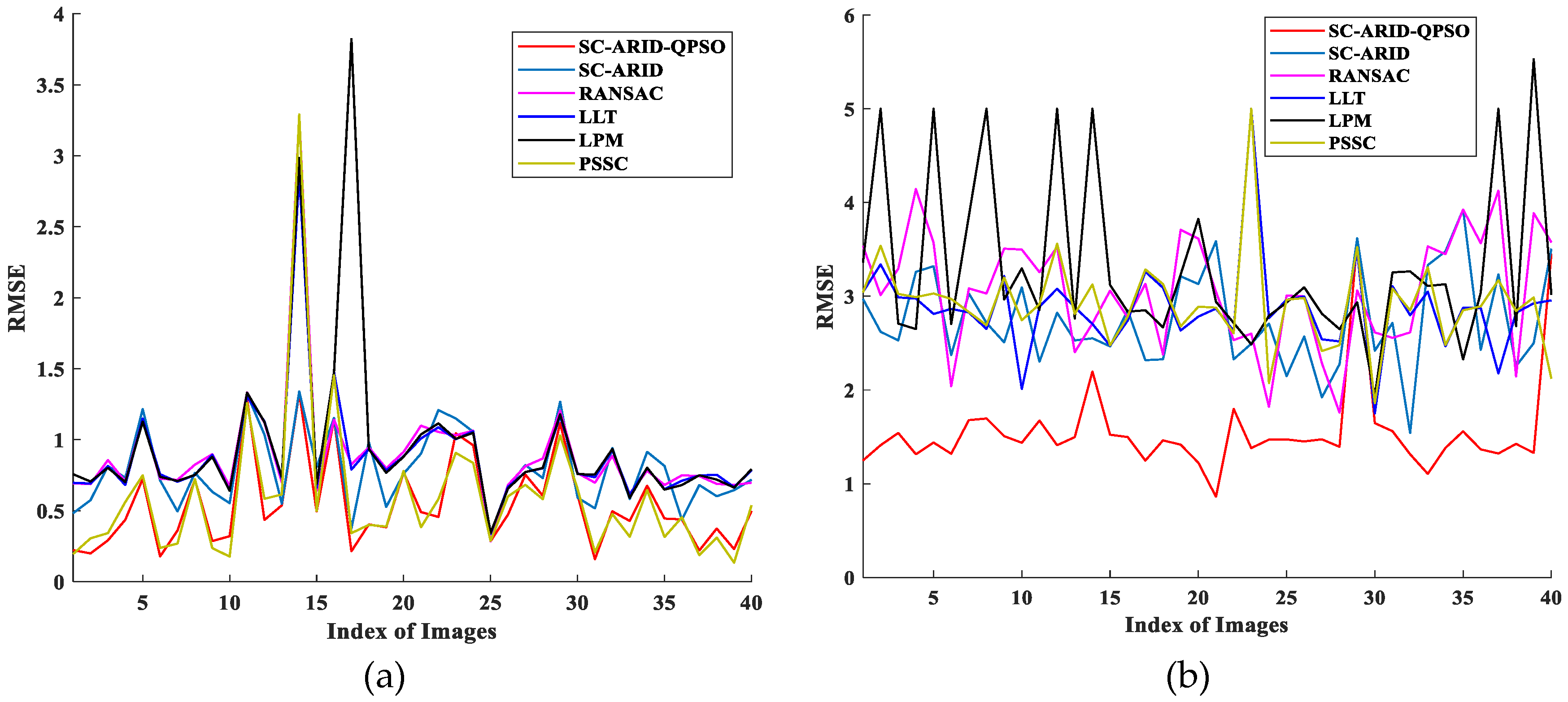
6.3. Comparative Analysis on Registration Performance

The results in Section 5.1 and Section 5.2 validated the effectiveness of SC-ARID-QPSO. In this section, we performed experiments to evaluate the comparative analysis of SC-ARID-QPSO to SC-ARID and other four compared methods, Random sample consensus (RANSAC) [15], locally linear transforming (LLT) [18,56], Locality preserving matching (LPM) [19,20,57], and via progressive sparse spatial consensus (PSSC) [21,58]. For fairness of comparison, SIFT feature extraction and SAD feature matching method were used. As shown in Figure 9a, the RMSEs of SC-ARID-QPSO were almost smaller than 1.5 pixels. Compared with SC-ARID the final registration accuracy obtained by the parameter optimization in Component II can be improved and resulted in smaller error. In addition, compared with the RMSE curves plotted in Figure 9a, the RMSEs of all methods for data with perspective deformation in dataset B are relatively larger as shown in Figure 9b. However, in comparison with SC-ARID and other four algorithms, SC-ARID-QPSO obtained significantly better results than the five compared algorithms. The RMSEs of most images produced by SC-ARID-QPSO were less than two pixels, compared to SC-ARID and the other four compared algorithms, which had RSMEs mostly around three pixels in Figure 9b.

7. Discussion

According to Figure 3 and Figure 6 and Component I in Table 1 and Table 2, the consistent feature set selection results from different criteria with spatial consistency show that the selection strategy using ARID as a metric can also evaluate the accuracy of the registration parameters accurately and robustly. As shown by the three simulated datasets and three real datasets, the consistent feature sets in Component I selected by SC-ARID were relatively better that by RANSAC and better or similar to that selected by SC-MI and SC-RMI. The selected feature set directly affects the registration accuracy, which will also generate a better set of initial particle swarms for the subsequent QPSO.

Combining the iterative curves in Figure 4 and Figure 7 and Component II in Table 1 and Table 2, the registration parameters obtained by SC-ARID-QPSO, SC-RMI-QPSO, and SC-MI-QPSO are relatively better or similar to the parameters by RS-ARID-QPSO, RS-RMI-QPSO, and RS-MI-QPSO. For the ARID-based method, the obtained parameter initialization could yield relatively better final results. In addition, it can be seen from the iterative curves in Figure 4 and Figure 7 that there was a decreasing tendency in registration error during the process of minimizing ARID. The iterative performance of the six methods and the final RMSE-based position accuracy demonstrated that the initialization of the registration parameters affected the registration accuracy to some extent. In addition, optimization algorithm and SV/DVs are another two key factors that had significant impact on the final registration parameters. Based on the above experimental results and analysis, the proposed SC with SV/DV via QPSO was shown to be effective and obtain good performance. The results validated the effectiveness and accuracy of the proposed cascaded registration system as well as the proposed ARID criterion.

By virtue of the above validation experiments, SC-ARID-QPSO performed better than SC-ARID and RANSAC to a certain degree. Because the performance of a feature-based method largely depends on the quality of extracted features, SC-ARID-QPSO can have relatively good performance. This is because the registration accuracy is not much affected by the original extracted feature set even though the ARID-based parameter optimization via QPSO uses the initialized parameters obtained in Component I.

Figure 9 shows these comparative experimental results to demonstrate the effectiveness and superiority of SC-ARID-QPSO to RANSAC, LLT, LPM, and PSSC for registering both satellite and aerial optical remote sensing images with affine or perspective transformations. In Figure 9a, the SC-ARID method obtained relatively better registration results compared to other algorithms which validated the performance of SC-ARID, and ARID-minimized parameter optimization could further reduce the final registration error. This curve also showed that FBMs could obtain good results for image registration of affine deformation with the RMSE values lower than 1.5 pixels. Nevertheless, ARID-minimized parameter optimization could produce results with higher accuracy although it may be somewhat affected by the initialization parameters. In Figure 9b, the registration errors of experiments on dataset B were larger than those on dataset A. This was because dataset B is generated by projection deformation and the image resolution is relatively higher than the images in dataset A. Compared to other four methods, SC-ARID-QPSO could still obtain better results. In practical applications, it is acceptable to obtain a registration error of less than 1.5 pixels for an image with a resolution of 0.3 m.

As for computational complexity, SC-ARID-QPSO can be discussed in two aspects, the consistent feature set selection in Component I and the objective function minimization via QPSO for parameter optimization in Component II. In the Component I, the factors that affect the running time of SC-ARID are (a) the number of consistent feature sets, N_SC; and (b) the computing time of metrics, denoted by t_ARID. In Component II, the factors contributed to the running time of SC-ARID-QPSO are (a) the number of iterations, N_iter; (b) the dimensionality of a particle, D defined by the type of the used transformation matrix; and (c) t_ARID. Although the values of N_iter and N_SC are unknown, the maximum values of these variables in the conducted experiments were set to 100. Among them, t_ARID is the primary factor to be affected by the image size. In order to further demonstrate the computational complexity, the time of calculating DV for each consistent feature set and the time of running a single iteration are used for illustration. For data set A, an image pair with a size of 512 × 512 registered by SC-ARID-QPSO required 0.85 s in calculating DV for each consistent feature set in Component I, and 11.47 s in a single-run iteration in Component II. For other compared methods, RANSAC, LLT, LPM, and PSSC took 13.26 s, 6.5 s, 4.68 s, and 3.48 s, respectively. The code used to conduct comparisons is publicly available in [56,57,58]. Generally speaking, ABMs run longer time than FBMs because ABMs need to obtain the registration parameters through searching by template window sliding or parameter optimization methods. Nonetheless, as mentioned above, ABMs can achieve higher registration accuracy than FBMs. Since the proposed ARID was developed to calculate the information divergency of regional intensity information, its future work can look into its design rationale to develop more robust and accuracy metrics, and regional intensity information can be replaced by regional descriptor.

8. Conclusions

This paper develops a two-component cascaded registration method based on spatial consistency and average regional information divergency, to be called spatial-consistency (SC) and average regional information divergence (ARID) minimization via quantum-behaved particle swarm optimization (SC-ARID-QPSO). As expected, SC-ARID-QPSO produces better positional accuracy than other existing registration algorithms, for example, RANSAC [2], LLT [18], LPM [19,20], and PSSC [21]. Several contributions which are not found in [41] are summarized as follows.

• A new measure, called average regional information divergency (ARID), is specifically designed to calculate the discrepancy between the registration parameters.
• SC-ARID-QPSO, using ARID to select a consistent feature set in Component I as well as to optimize registration parameters in Component II, provides a novel approach as a new AFBM.
• The feature extraction method and parameter optimization algorithm used in SC-ARID-QPSO can be replaced by better feature extraction methods and optimization algorithms. Under certain extreme situations, where there are no more than three or more pairs of correctly matched feature pairs among initial SIFT feature pairs, other modified better feature extraction methods can be used to replace SIFT. In this case, the framework of SC-ARID-QPSO is still applicable.

References

1. Zitová, B.; Flusser, J. Image registration methods: A survey. Image Vis. Comput. 2003, 21, 977–1000. [Google Scholar] [CrossRef] [Green Version]
2. Lowe, D.G. Distinctive image features from scale-invariant keypoints. Int. J. Comput. Vis. 2004, 60, 91–110. [Google Scholar] [CrossRef]
3. Sedaghat, A.; Mokhtarzade, M.; Ebadi, H. Uniform robust scale-invariant feature matching for optical remote sensing images. IEEE Trans. Geosci. Remote Sens. 2011, 49, 4516–4527. [Google Scholar] [CrossRef]
4. Paul, S.; Pati, U.C. Remote sensing optical image registration using modified uniform robust SIFT. IEEE Geosci. Remote Sens. Lett. 2016, 13, 1300–1304. [Google Scholar] [CrossRef]
5. Xiang, Y.; Wang, F.; You, H. OS-SIFT: A robust SIFT-like algorithm for high-resolution optical-to-SAR image registration in suburban areas. IEEE Trans. Geosci. Remote Sens. 2018, 56, 3078–3090. [Google Scholar] [CrossRef]
6. Chang, H.; Wu, G.; Chiang, M. Remote sensing image registration based on modified SIFT and feature slope grouping. IEEE Geosci. Remote Sens. Lett. 2019, 16, 1363–1367. [Google Scholar] [CrossRef]
7. Sedaghat, A.; Mohammadi, N. Uniform competency-based local feature extraction for remote sensing images. ISPRS J. Photogramm. Remote Sens. 2018, 135, 142–157. [Google Scholar] [CrossRef]
8. Bay, H.; Ess, A.; Tuytelaars, T.; Gool, L.V. Speeded-up robust features (SURF). Comput. Vis. Image Underst. 2007, 110, 346–359. [Google Scholar] [CrossRef]
9. Mikolajczyk, K.; Schmid, C. A performance evaluation of local descriptors. IEEE Trans. Pattern Anal. Mach. Intell. 2005, 27, 1615–1630. [Google Scholar] [CrossRef] [Green Version]
10. Tola, E.; Lepetit, V.; Fua, P. DAISY: An efficient dense descriptor applied to wide-baseline stereo. IEEE Trans. Pattern Anal. Mach. Intell. 2010, 32, 815–830. [Google Scholar] [CrossRef] [Green Version]
11. Sedaghat, A.; Ebadi, H. Remote sensing image matching based on adaptive binning SIFT descriptor. IEEE Trans. Geosci. Remote Sens. 2015, 53, 5283–5293. [Google Scholar] [CrossRef]
12. Chen, J.; Tian, J.; Lee, N.; Zheng, J.; Smith, R.T.; Laine, A.F. A partial intensity invariant feature descriptor for multimodal retinal image registration. IEEE Trans. Biomed. Eng. 2010, 57, 1707–1718. [Google Scholar] [CrossRef] [Green Version]
13. Sedaghat, A.; Ebadi, H. Distinctive order based self-similarity descriptor for multi-Sensor remote sensing image matching. ISPRS J. Photogramm. Remote Sens. 2015, 108, 62–71. [Google Scholar] [CrossRef]
14. Sedaghat, A.; Mohammadi, N. Illumination-robust remote sensing image matching based on oriented self-similarity. ISPRS J. Photogramm. Remote Sens. 2019, 153, 21–35. [Google Scholar] [CrossRef]
15. Fischler, M.A.; Bolles, R.C. Random sample consensus: A paradigm for model fitting with applications to image analysis and automated cartography. Commun. ACM 1980, 24, 381–395. [Google Scholar] [CrossRef]
16. Song, Z.; Zhou, S.; Guan, J. A novel image registration algorithm for remote sensing under affine transformation. IEEE Trans. Geosci. Remote Sens. 2014, 52, 4895–4912. [Google Scholar] [CrossRef]
17. Wu, Y.; Ma, W.P.; Gong, M.G.; Su, L.Z.; Jiao, L.C. A novel point-matching algorithm based on fast sample consensus for image registration. IEEE Geosci. Remote Sens. Lett. 2015, 12, 43–47. [Google Scholar] [CrossRef]
18. Ma, J.Y.; Zhou, H.B.; Zhao, J.; Gao, Y.; Jiang, J.J.; Tian, J.W. Robust feature matching for remote sensing image registration via locally linear transforming. IEEE Trans. Geosci. Remote Sens. 2015, 53, 6469–6481. [Google Scholar] [CrossRef]
19. Ma, J.Y.; Zhao, J.; Jiang, J.J.; Zhou, H.B. Locality preserving matching. Int J. Comput. Vis. 2019, 127, 512–531. [Google Scholar] [CrossRef]
20. Ma, J.Y.; Zhao, J.; Jiang, J.J.; Zhou, H.B. Locality preserving matching. In Proceedings of the International Joint Conference on Artificial Intelligence (IJCAI), Melbourne, VIC, Australia, 19–25 August 2017; pp. 4492–4498. [Google Scholar]
21. Ma, Y.; Wang, J.; Xu, H.; Zhang, S.; Mei, X.; Ma, J. Robust image feature matching via progressive sparse spatial consensus. IEEE Access 2017, 5, 24568–24579. [Google Scholar] [CrossRef]
22. Maes, F.; Collignon, A.; Vandermeulen, D.; Marchal, G.; Suetens, P. Multimodality image registration by maximization of mutual information. IEEE Trans. Med. Imaging 1997, 16, 187–198. [Google Scholar] [CrossRef] [PubMed] [Green Version]
23. Yi, Z.; Cao, Z.G.; Yang, X. Multi-spectral remote image registration based on SIFT. Electron. Lett. 2008, 44, 107–108. [Google Scholar] [CrossRef]
24. Liang, J.; Liu, X.P.; Huang, K.N.; Li, X.; Wang, D.G.; Wang, X.W. Automatic registration of multisensor images using an integrated spatial and mutual information (SMI) metric. IEEE Trans. Geosci. Remote Sens. 2014, 52, 603–615. [Google Scholar] [CrossRef]
25. Russakoff, D.B.; Tomasi, G.; Rohlfing, T. Image similarity using mutual information of regions. Eur. Conf. Comput. Vis. 2004, 3023, 596–607. [Google Scholar]
26. Li, L.X. The Registration and Fusion of Multi-sensor Images Based on Mutual Information. Master’s Thesis, University of Electronic Science and Technology of China, Chengdu, China, 2013. [Google Scholar]
27. Wong, A.; Clausi, D.A. ARRSI: Automatic registration of remote sensing images. IEEE Trans. Geosci. Remote Sens. 2007, 45, 1483–1493. [Google Scholar] [CrossRef]
28. Navy, P.; Page, V.; Grandchamp, E.; Desachy, J. Matching two clusters of points extracted from satellite images. Pattern Recognit. Lett. 2006, 27, 268–274. [Google Scholar] [CrossRef] [Green Version]
29. Rueckert, D.; Clarkson, M.J.; Hill, D.L.G.; Hawkes, D.J. Non-rigid registration using higher-order mutual information. In Proceedings of the Medical Imaging 2000: Image Processing Proceedings SPIE, San Diego, CA, USA, 14 February 2000; Volume 3979, pp. 438–447. [Google Scholar]
30. Pluim, J.P.W.; Maintz, J.B.A.; Viergever, M.A. Image registration by maximization of combined mutual information and gradient information. IEEE Trans. Med. Imaging 2000, 19, 809–814. [Google Scholar] [CrossRef]
31. Cole-Rhodes, A.A.; Johnson, K.L.; LeMoigne, J.; Zavorin, I. Multiresolution registration of remote sensing imagery by optimization of mutual information using a stochastic gradient. IEEE Trans. Image Process. 2003, 12, 1495–1511. [Google Scholar] [CrossRef]
32. Kern, J.P.; Pattichis, M.S. Robust multispectral image registration using mutual-information models. IEEE Trans. Geosci. Remote Sens. 2007, 45, 1494–1505. [Google Scholar] [CrossRef]
33. Chen, H.M.; Varshney, P.K.; Arora, M.K. Performance of mutual information similarity measure for registration of multitemporal remote sensing images. IEEE Trans. Geosci. Remote Sens. 2003, 41, 2445–2454. [Google Scholar] [CrossRef]
34. Studholme, C.; Hill, D.L.G.; Hawkes, D.J. An overlap invariant entropy measure of 3D medical image alignment. Pattern Recognit. 1999, 32, 71–86. [Google Scholar] [CrossRef]
35. Johnson, K.; Cole-Rhodes, A.; Zavorin, I.; Moigne, J.L. Mutual information as a similarity measure for remote sensing image registration. Proc. SPIE 2001, 4383, 51–61. [Google Scholar]
36. Gong, M.G.; Zhao, S.M.; Jiao, L.C.; Tian, D.Y.; Wang, S. A novel coarse-to-fine scheme for automatic image registration based on SIFT and mutual information. IEEE Trans. Geosci. Remote Sens. 2014, 52, 4328–4438. [Google Scholar] [CrossRef]
37. Zhao, L.Y.; Lv, B.Y.; Li, X.R.; Chen, S.H. Multi-source remote sensing image registration based on scale-invariant feature transform and optimization of regional mutual information. Acta Phys. Sin. Chin. Ed. 2015, 64, 124204. [Google Scholar]
38. Chen, S.H.; Li, X.R.; Zhao, L.Y.; Yang, H. Medium-low resolution multisource remote sensing image registration based on SIFT and robust regional mutual information. Int. J. Remote Sens. 2018, 39, 3215–3242. [Google Scholar] [CrossRef]
39. Ye, Y.X.; Shan, J. A local descriptor based registration method for multispectral remote sensing images with non-linear intensity differences. ISPRS J. Photogramm. Remote Sens. 2014, 90, 83–95. [Google Scholar] [CrossRef]
40. Yang, H.; Li, X.R.; Zhao, L.Y.; Chen, S.H. A novel coarse-to-fine scheme for remote sensing image registration based on SIFT and phase correlation. Remote Sens. 2019, 11, 1833. [Google Scholar] [CrossRef] [Green Version]
41. Chen, S.H.; Zhong, S.W.; Xue, B.; Li, X.R.; Zhao, L.Y.; Chang, C.-I. Iterative Scale-Invariant Feature Transform for Remote Sensing Image Registration. IEEE Trans. Geosci. Remote Sens. 2020, 1–22. [Google Scholar] [CrossRef]
42. Gharbia, R.; Ahmed, S.A.; Hassanien, A.E. Remote Sensing Image Registration Based on Particle Swarm Optimization and Mutual Information; Springer: New Delhi, India, 2015; Volume 127, pp. 399–408. [Google Scholar]
43. Zhuang, Y.W.; Gao, K.; Miu, X.H.; Han, L.; Gong, X.M. Infrared and visual image registration based on mutual information with a combined particle swarm optimization Powell search algorithm. Opt. Int. J. Light Electron. Opt. 2016, 127, 188–191. [Google Scholar] [CrossRef]
44. Xia, K.M.; Chen, X.Z.; Guo, G.G. Fast Algorithm for Simulated Annealing Applied to Registering of Noisy Images. J. Shanghai Univ. 2003, 9, 392. [Google Scholar]
45. Liu, P.; Zhou, J.; Luo, D.Z.; Kai, D.U. Research on IR and Visual Image Registration Based on Mutual Information and Ant Colony Algorithm. Microcomput. App. 2008, 29, 53–58. [Google Scholar]
46. Sun, T.H. Applying particle swarm optimization algorithm to roundness measurement. Expert Syst. Appl. 2009, 36, 3428–3438. [Google Scholar] [CrossRef]
47. Sun, J.; Feng, B.; Xu, W.B. Particle swarm optimization with particles having quantum behavior. In Proceedings of the 2004 Congress on Evolutionary Computation CEC2004, Portland, OR, USA, 19–23 June 2004; pp. 325–331. [Google Scholar]
48. Sun, J.; Feng, B.; Xu, W.B. Adaptive Parameter Control for Quantum-behaved Particle Swarm Optimization on Individual Level. In Proceedings of the 2005 IEEE International Conference on Systems, Man and Cybernetics, Hawaii, HI, USA, 10–12 October 2005; p. 30493054. [Google Scholar]
49. Chang, C.-I. Hyperspectral Imaging: Techniques for Spectral Detection and Classification; Kluwer Academic/Plenum Publishers: New York, NY, USA, 2003. [Google Scholar]
50. Chang, C.-I. An information-theoretic approach to spectral variability, similarity, and discrimination for hyperspectral image analysis. IEEE Trans. Inf. Theory 2000, 46, 1927–1932. [Google Scholar] [CrossRef] [Green Version]
51. ENVI Image Analysis Software (5.2 version). L3HARRIS Geospatial. Available online: https://www.harrisgeospatial.com/Software-Technology/ENVI (accessed on 15 October 2014).
52. UC Merced Land Use Dataset. Available online: http://140.112.27.140/wp-content/uploads/2018/12/Datasets.zip (accessed on 5 December 2018).
53. High-Resolution Orthoimagery Data. Available online: http://weegee.vision.ucmerced.edu/datasets/landuse.html (accessed on 28 October 2010).
54. USGS. Earth Explorer. Available online: https://earthexplorer.usgs.gov/ (accessed on 28 August 2016).
55. Yang, Y.; Newsam, S. Bag-of-visual-words and spatial extensions for land-use classification. In Proceedings of the ACM SIGSPATIAL International Conference on Advances in Geographic Information Systems (ACM GIS), San Jose, CA, USA, 2–5 November 2010. [Google Scholar]
56. Matlab Code of LLT. Available online: https://github.com/jiayi-ma/LLT (accessed on 29 September 2018).
57. Matlab Code of LPM. Available online: https://github.com/jiayi-ma/LPM (accessed on 16 March 2019).
58. Matlab Code of PSSC. Available online: https://github.com/JiahaoPlus/PSSC (accessed on 31 December 2018).
Figure 1. A graphic diagram of implementing spatial-consistency and average regional information divergence minimization via quantum-behaved particle swarm optimization (SC-ARID-QPSO).
Remotesensing 12 03066 g001
Figure 2. A block diagram of implementing SC-ARID-QPSO.
Remotesensing 12 03066 g002
Figure 3. Similarity value (SV) plots for simulated image 1. (a) mutual information (MI) plots; (b) regional mutual information (RMI) plots. (Index is 24 and SVMI = 0.1491) (Index is 10 and SVRMI = 0.9351); (c) ARID plots; (d) Number of features in each feature set. (Index is 24 and discrepancy value (DV)ARID = 0.1138) (Index is 2 and NInner = 11); (e) Root mean square error RMSE plots (RMSE2 = 1.976, RMSE10 = 1.746, RMSE24 = 1.712).
Remotesensing 12 03066 g003aRemotesensing 12 03066 g003b
Figure 4. Iterative plots for simulated images 1–3. (a) SVs and RMSE plots for simulated image 1. (b) SVs and RMSE plots for simulated image 2. (c) SVs and RMSE plots for simulated image 3.
Remotesensing 12 03066 g004aRemotesensing 12 03066 g004b
Figure 5. Checkboard mosaic images for simulated images 1–3 based on SC-MI-QPSO, SC-RMI-QPSO, and SC-ARID-QPSO respectively. (ac) Checkboard mosaic images for simulated image 1. (df) Checkboard mosaic images for simulated image 2. (gi) Checkboard mosaic images for simulated image 3.
Remotesensing 12 03066 g005aRemotesensing 12 03066 g005b
Figure 6. SV plots for real image 1. (a) MI plots; (b) RMI plots (Index is 14 and SVMI = 0.0726) (Index is 56 and SVRMI = 1.006); (c) ARID plots; (d) Number of features in each feature set (Index is 56 and SVARID = 0.0689) (Index is 32 and NInner = 58); (e) RMSE plots (RMSE14 = 1.355, RMSE32 = 1.592, RMSE56 = 1.401).
Remotesensing 12 03066 g006aRemotesensing 12 03066 g006b
Figure 7. Iterative plots for real images 1–3. (a) SVs and RMSE plots for real image 1. (b) SVs and RMSE plots for real image 2. (c) SVs and RMSE plots for real image 3.
Remotesensing 12 03066 g007aRemotesensing 12 03066 g007b
Figure 8. Checkboard mosaic images for real images 1–3 based on SC-MI-QPSO, SC-RMI-QPSO, and SC-ARID-QPSO, respectively. (ac) Checkboard mosaic images for real image 1. (df) Checkboard mosaic images for real image 2. (gi) Checkboard mosaic images for real image 3.
Remotesensing 12 03066 g008
Figure 9. Comparison of final RMSEs using SC-ARID-QPSO, SC-ARID, RANSAC, LLT, LPM and PSSC with different transformation. (a) Set-A data sets with affine deformation; (b) Set-B data sets with perspective deformation.
Remotesensing 12 03066 g009