Article

Detection of Chlorophyll a and CDOM Absorption Coefficient with a Dual-Wavelength Oceanic Lidar: Wavelength Optimization Method

1
Ningbo Research Institute, State Key Laboratory of Modern Optical Instrumentation, College of Optical Science and Engineering, Zhejiang University, Hangzhou 310027, China
2
Ocean College, Zhejiang University, Zhoushan 316021, China
3
Shanghai Institute of Optics and Fine Mechanics, Chinese Academy of Science, Shanghai 201800, China
4
National Laboratory for Marine Science and Technology, Qingdao 266100, China
*
Author to whom correspondence should be addressed.
Remote Sens. 2020, 12(18), 3021; https://doi.org/10.3390/rs12183021
Submission received: 27 July 2020 / Revised: 4 September 2020 / Accepted: 11 September 2020 / Published: 16 September 2020
(This article belongs to the Section Ocean Remote Sensing)

Abstract

:
To overcome the retrieval problems in complex water, dual working wavelengths are required instead of a single wavelength in oceanic lidar. The wavelength optimization method of detecting chlorophyll a and Colored Dissolved Organic Matter (CDOM) absorption coefficient with a dual-wavelength lidar is studied in this paper. The inversion methods of chlorophyll a and CDOM absorption are developed based on the water absorption characteristics, which then lead to the inversion error equations. The effects of the wavelength on the inversion errors are studied. For the case in which λ1 and λ2 are both random, the errors are relatively small when λ1 is chosen between 420 and 560 nm and λ2 is selected under 420 nm. For the case in which λ1 is fixed at 532 nm, the errors generally decrease with decreasing λ2, with minimums around 300 and 356–360 nm under different water conditions. The wavelength optimization method discussed in this paper and the penetration depth criterion will be beneficial to the design of the dual-wavelength lidar.

1. Introduction

The ocean covers more than 71% of the earth and plays a highly significant role in the global ecosystem and climate change [1,2]. Several methods are employed for detecting the optical properties of the ocean’s interior. In situ methods, such as the transmissometer and scattering meter, can obtain the marine information accurately, yet are limited by efficiency [3]. The ocean color remote sensing methods measured from the plane or satellite, like Moderate-Resolution Imaging Spectroradiometer, are able to collect global data efficiently over the long term [4]. Nevertheless, the limited information about the depth and dependence on the natural light restricts its applications. Acoustics are widely used for profiling the seawater, but they can only work on underwater platforms, due to a high loss at the air-water interface. Lidar is an effective method that breaks through the above limitations, which is attractive due to its high temporal-spatial resolution and observation ability of deep water. For example, Schulien et al. demonstrated that airborne high-spectral-resolution Lidar (HSRL) measurements were able to accurately measure to 2.5–3 optical depths at 1 m resolution [5]. Thus far, oceanic lidars have been employed in detecting fishes, phytoplankton layers, and internal waves, etc., in the upper ocean [6].
At present, a single wavelength is widely employed to measure ocean properties using the lidar technique. As the second-harmonic wavelength of the Nd:YAG laser, 532 nm is generally employed as the working wavelength. For example, Cloud Aerosol Lidar with Orthogonal Polarization (CALIOP) is a simple elastic backscatter lidar with emissions at 532 and 1064 nm. However, for 1064 nm, -its in-water attenuation is too large to provide useful subsurface information [7]. Hair et al. used the HSRL at 532 nm, a more advanced lidar that can measure the attenuation and backscattering independently [7,8]. Liu et al. [9], Collister et al. [10], Churnside et al. [11], and Liu et al. [12] also used 532 nm as the working wavelength. If the seawater includes only water molecules and phytoplankton, the single-wavelength lidar can obtain chlorophyll a using the existing bio-optical model. However, colored dissolved organic matter (CDOM) also exist in all ocean waters. Thus chlorophyll a cannot be accurately obtained by using only one wavelength.
Lidar that employs more than one wavelength is a possible method to solve the simultaneous retrieval problem of chlorophyll a and CDOM absorption. Although Gray et al. [13] developed a dual-wavelength lidar at 473 and 532 nm and Strait et al. [14] developed a lidar with a wavelength tunable from 410 to 700 nm, discrimination of chlorophyll a and CDOM absorption has not been realized. Hoge put forward the idea of the dual-wavelength lidar to solve this problem [15] and Hostetler et al. proposed to collect measurements at 355 nm and 532 nm [7]. At present, determining the best dual-wavelengths through a quantitative analysis is beneficial for the ocean lidar community. In this paper, the retrieval equations and the error transfer formulas of CDOM absorption coefficients and chlorophyll a are derived considering a dual-wavelength lidar. The effects of wavelength on errors are analyzed and the wavelength selection method of the dual-wavelength lidar is proposed.
The paper is constructed as follows. In Section 2, an introduction of the retrieval equations and error transfer formulas are described. In Section 3, the wavelength effects on the errors and selection method of the wavelength are presented. In Section 4, we discuss the other factors that might influence the wavelength selection and retrieval accuracy. Concluding remarks are summarized in the last section.

2. Method

Lidar signals contain 2 seawater optical properties, which are 180-degree volume scattering function and lidar attenuation coefficient. Several methods can be used to retrieve the 2 properties from the original signals. For elastic lidar, when the water column is well mixed, the slope method can be used. When the type of particles in the water does not change with depth, the Fernald method is better [16,17]. When changes in the depth profile of the optical properties are not too extreme, it is better to utilize the perturbation method [18,19,20]. For HSRL, the 2 properties can be retrieved independently [6,21]. The backscattering coefficient can be retrieved from the 180-degree volume scattering function through a conversion factor [8].
Gordon [22] indicated that the lidar attenuation coefficient could be regarded as the diffuse attenuation coefficient using the Kullenberg phase function if the field of view was large enough [23]. According to simulation results obtained by Lee, the diffuse attenuation coefficient can be written as a function of the absorption coefficient and the backscattering coefficient [24]. Therefore, the absorption coefficient can be derived from the lidar-measured diffuse attenuation coefficient and the backscattering coefficient. In addition, Liu found the seawater scattering phase function can be expressed in a two-term Henyey–Greenstein form through simulation. Furthermore, the lidar attenuation coefficient can be directly written as a function of the absorption coefficient and the backscattering coefficient [25]. Therefore, the absorption coefficient can be derived from the lidar attenuation coefficient and the backscattering coefficient. In either case, from the existing theory, the absorption coefficient can be retrieved using the oceanic lidar. Furthermore, for dual-wavelength lidar, the absorption coefficients at the 2 wavelengths can be measured simultaneously.

2.1. Inversion Formula

The main components of the water body included seawater, particles, and CDOM. Each component makes a distinct contribution to the total absorption coefficient, which can be written as
a ( λ ) = a w ( λ ) + a p ( λ ) + a g ( λ )
where a w ( λ ) is the absorption coefficient of pure seawater, which is only related to the wavelength and has been measured [26]. a p ( λ ) is the absorption coefficient of the particles, including phytoplankton and a few detritus, and is mainly contributed by chlorophyll a. It can be estimated by [27]
a p ( λ ) = A ( λ ) × C E ( λ )
where A ( λ ) is the specific absorption coefficient of chlorophyll a, and the unit is m−1. C is the concentration of chlorophyll a, and is expressed in μg L−1. E ( λ ) is the index absorption coefficient of chlorophyll a. The data of A ( λ ) and E ( λ ) used in this paper comes from Ocean Optics Web Book [28]. a g ( λ ) is the absorption coefficient of CDOM, which shows an exponential decay with λ increasing in the range of 200–800 nm, that is [29]
a g ( λ ) = a g ( λ 0 ) × exp [ S ( λ λ 0 ) ]
where S is the spectral absorption slope, and the unit is nm−1, a g ( λ 0 ) is the absorption coefficient of CDOM at the reference wavelength λ0, which is a representation of the CDOM concentration [30]. It is worth noting that the absorption curves of all detritus and CDOM can be described by exponential absorption models [31], and the curves are very similar or even difficult to distinguish. Here we do simplification and express the absorption of both with a g ( λ ) , which will be meaningful when the absorption of detritus cannot be completely considered in a p ( λ ) .
The spectral characteristics of the absorption coefficient in the water are shown in Figure 1. The contributions of the pure water particles, and CDOM are shown in Figure 1a, where λ0 is set at 532 nm, C is 20 μg L−1, a g ( λ 0 ) is 0.0772 m−1, and S is 0.014 nm−1. a w ( λ ) is small if the wavelength is smaller than 550 nm but increases rapidly between 550 and 700 nm. For the particles, there is a primary peak at 440 nm, more significant than the secondary peak near 680 nm. Besides, particles have an elevated absorption near 310 nm, which is likely due to mycosporine-like amino acids (MAAs). MAAs are UV absorbing, compounds that contain either an aminocylcohexenone or aminocylcohexenimine unit. MAAs have been shown to be released from phytoplankton grown in cultures [32]. MAAs have also been observed in 83% of the samples analyzed with concentrations ranging from 0 to 2.75 μM in the particulate organic matter (POM) in ocean samples [33]. The CDOM absorption decreases exponentially with the increasing wavelength. The absorption trends of CDOM and particles were opposite between 360 and 440 nm and 550 and 680 nm but similar between 440 and 550 nm and 310 and 360 nm, respectively. The same trend was not conducive to distinguishing the 2 components. Figure 1b shows the total absorption curves under different C and a g ( λ 0 ) . At shorter wavelengths, particles and CDOM contributed more to the absorption signal.
According to Equations (1)–(3), the dual-wavelength lidar can obtain absorption coefficients at λ1 and λ2, which are,
{ a ( λ 1 ) = a w ( λ 1 ) + A ( λ 1 ) × C E ( λ 1 ) + a g ( λ 0 ) × exp [ S ( λ 1 λ 0 ) ] a ( λ 2 ) = a w ( λ 2 ) + A ( λ 2 ) × C E ( λ 2 ) + a g ( λ 0 ) × exp [ S ( λ 2 λ 0 ) ]
In Equation (4), a w ( λ ) varies little with the changes of other components of the water body, thus it can be considered as known. A ( λ ) , E ( λ ) and S are assumed to be known. C can be expressed with a g ( λ 0 ) using the first equation of Equation (4), then be placed into the second equation. An implicit function of C is obtained. The implicit function of a g ( λ 0 ) can be obtained the same way. Therefore the critical parameters of chlorophyll a and CDOM, C and a g ( λ 0 ) , can be expressed as, respectively,
{ [ a ( λ 1 ) a w ( λ 1 ) A ( λ 1 ) × C E ( λ 1 ) ] × exp ( S λ 1 ) = [ a ( λ 2 ) a w ( λ 2 ) A ( λ 2 ) × C E ( λ 2 ) ] × exp ( S λ 2 ) { a ( λ 1 ) a w ( λ 1 ) a g ( λ 0 ) exp [ S ( λ 1 λ 0 ) ] A ( λ 1 ) } E ( λ 2 ) = { a ( λ 2 ) a w ( λ 2 ) a g ( λ 0 ) exp [ S ( λ 2 λ 0 ) ] A ( λ 2 ) } E ( λ 1 )
According to Equation (5), C and a g ( λ 0 ) can be calculated using the dual-wavelength lidar and the known absorption spectrum of chlorophyll a and CDOM. Unfortunately, since Equation (5) is a transcendental equation, only numerical solutions of C and a g ( λ 0 ) can be obtained, rather than their analytical expressions.

2.2. Error Analysis

Due to the instrumental and environmental factors, measured errors of total absorption coefficients at λ1 and λ2 were unavoidable. Therefore, it was necessary to evaluate the effects of these measured errors on the retrieval accuracy of C and a g ( λ 0 ) . The classic error propagation law can be utilized here to study the chlorophyll error as follows
ε C 2 = [ ε C a ( λ 1 ) ] 2 + [ ε C a ( λ 2 ) ] 2
where ε C is the total relative error of the chlorophyll, ε C a ( λ 1 ) and ε C a ( λ 2 ) are relative errors of the chlorophyll contributed by the measurement errors of a ( λ 1 ) and a ( λ 2 ) , respectively, those are,
{ [ ε C a ( λ 1 ) ] 2 = [ C C a ( λ 1 ) ] 2 [ σ a ( λ 1 ) ] 2 = [ Δ a ( λ 1 ) ] 2 × { 1 + a w ( λ 1 ) + a g ( λ 0 ) exp [ S ( λ 0 λ 1 ) ] A ( λ 1 ) × C E ( λ 1 ) E ( λ 1 ) E ( λ 2 ) × A ( λ 2 ) A ( λ 1 ) × C E ( λ 2 ) E ( λ 1 ) × exp [ S ( λ 2 λ 1 ) ] } 2 [ ε C a ( λ 2 ) ] 2 = [ C C a ( λ 2 ) ] 2 [ σ a ( λ 2 ) ] 2 = [ Δ a ( λ 2 ) ] 2 × { 1 + a w ( λ 2 ) + a g ( λ 0 ) exp [ S ( λ 0 λ 2 ) ] A ( λ 2 ) × C E ( λ 2 ) E ( λ 2 ) E ( λ 1 ) × A ( λ 1 ) A ( λ 2 ) × C E ( λ 1 ) E ( λ 2 ) × exp [ S ( λ 1 λ 2 ) ] } 2
where σ and Δ are the absolute and relative errors of the corresponding quantity. Equation (7) is derived using the differential calculation of Equation (5). Combining Equations (1)–(7), Equation (6) can be simplified as
ε C 2 = [ ( σ a ( λ 1 ) ) 2 + ( σ a ( λ 2 ) M g ) 2 ] × [ 1 a p ( λ 2 ) E ( λ 2 ) ] 2 × [ 1 M E M C M g ] 2
where M g = a g ( λ 1 ) / a g ( λ 2 ) , M C = a p ( λ 1 ) / a p ( λ 2 ) and M E = E ( λ 1 ) / E ( λ 2 ) . The first term means that the influence of σ a ( λ 2 ) is M g times that of σ a ( λ 1 ) , thus if M g > 1, it is more critical to reduce σ a ( λ 2 ) than σ a ( λ 1 ) for the chlorophyll retrieval. In the second term, E ( λ 2 ) has a smaller value at short wavelengths, while a p ( λ 2 ) has a larger value. Thus choosing the second wavelength within short wavelengths is beneficial to the second term. The third term shows that if M g M E M C or M g M E M C , which roughly means that the trends of the particles and CDOM absorption in Figure 1a are totally different, the retrieval error of chlorophyll could be significantly decreased.
Similarly, the total relative error of a g ( λ 0 ) is written as
ε a g ( λ 0 ) 2 = [ ε a g ( λ 0 ) a ( λ 1 ) ] 2 + [ ε a g ( λ 0 ) a ( λ 2 ) ] 2
where
{ [ ε a g ( λ 0 ) a ( λ 1 ) ] 2 = [ a g ( λ 0 ) a g ( λ 0 ) a ( λ 1 ) ] 2 [ σ a ( λ 1 ) ] 2 = [ Δ a ( λ 1 ) ] 2 × { 1 + a w ( λ 1 ) + A ( λ 1 ) × C E ( λ 1 ) a g ( λ 0 ) exp [ S ( λ 0 λ 1 ) ] 1 exp [ S ( λ 1 λ 2 ) ] × A ( λ 1 ) A ( λ 2 ) × E ( λ 1 ) E ( λ 2 ) × C E ( λ 1 ) E ( λ 2 ) } 2 [ ε a g ( λ 0 ) a ( λ 2 ) ] 2 = [ a g ( λ 1 ) a g ( λ 0 ) a ( λ 2 ) ] 2 [ σ a ( λ 2 ) ] 2 = [ Δ a ( λ 2 ) ] 2 × { 1 + a w ( λ 2 ) + A ( λ 2 ) × C E ( λ 2 ) a g ( λ 0 ) exp [ S ( λ 0 λ 2 ) ] 1 exp [ S ( λ 2 λ 1 ) ] × A ( λ 2 ) A ( λ 1 ) × E ( λ 2 ) E ( λ 1 ) × C E ( λ 2 ) E ( λ 1 ) } 2
Combining Equations (1)–(5) and (9)–(10), Equation (9) can be rewritten as
ε a g ( λ 0 ) 2 = [ σ a ( λ 1 ) + σ a ( λ 2 ) M C M E ] 2 × [ 1 a g ( λ 2 ) ] 2 × [ 1 M C M E M g ] 2
Equation (11) is similar to Equation (8). The first term means the influence of σ a ( λ 1 ) is more significant than that of σ a ( λ 2 ) if M C M E < 1. The second term means that a large a g ( λ 2 ) results in a small error. The third term shows the different trends of the particles and CDOM absorption could decrease the retrieval error.

3. Results

In this section, several steps will be used to illustrate the retrieval of the dual-wavelength lidar. The Monte Carlo (MC) method was used to verify the correctness of the theoretical model of Equations (8) and (11). Then, the effect of the dual-wavelength selection on retrieval errors was analyzed. Furthermore, the relationship between λ2 and error was analyzed when λ1 was fixed at 532 nm. Finally, the dual-wavelength lidar method was validated based on the in situ seawater absorption coefficients. Table 1 lists the input seawater optical properties in the following simulation. ag(532) was set at 0.01–0.05 m−1, C was set at 0.5–5.0 μg L−1 and S was set at 0.011–0.019 nm−1. According to global CDOM (ag(443)) and chlorophyll distribution, 0.01–0.05 m−1 for ag(532) and 0.5–5 μg L−1 for C have covered a large dynamic range [29,36]. Studies have shown that the S value of coastal seawater is usually between 0.011 and 0.018 nm−1 [37] and 0.014–0.019 nm1 [38].
The correctness of Equations (8) and (11) was verified by the MC method, as shown in Figure 2. λ1 = 532 nm and λ2 = 350 nm were selected to simulate all 7 cases in Table 1. The measurement error of bbp was 19.84%, and that of Kd was 17.63% in [5]. Besides, the error of Kd was 10.06% in [9]. Therefore, we set Δ a ( λ 1 ) and Δ a ( λ 2 ) at 20%. In Figure 2a,c, 500 MC results were plotted in red dots, the 3-σ results calculated by the theoretical model were plotted in the black dots, and the true values were plotted in the blue dots. Most of the MC results were within the 3-σ error range showing the great agreement between the theoretical model and the MC method. Notably, CE solved by Equation (5) contained negative numbers, resulting in the fact that C had an imaginary number solution, and thereby the red dots in Figure 2a cannot be exactly surrounded by 3-σ. In Figure 2b,d, the root mean squares of the relative errors of the MC results were plotted in red dots, and the theoretical errors were plotted in black dots. It shows that the MC results were very consistent with the theoretical results. Therefore, the theoretical model will be used for the following analysis, which largely decreases the computational costs.

3.1. Dual-Wavelength Analysis

Figure 3 shows the relationship between dual-wavelengths and relative errors. Mg, MC, and ME in Equations (8) and (11) were related to both λ1 and λ2. We set Δ a ( λ 1 ) and Δ a ( λ 2 ) at 20%, and other parameters as Case 1 in Table 1. The situation λ1 > λ2 instead of the situation λ1 < λ2 was considered to enhance the readability of Figure 3. The two situations were similar due to symmetry. Figure 3a,b show the effect of the dual-wavelength selection on C and ag(532). The black line indicates that inversion errors are 200%.
In Figure 3a, when λ1 >560 nm or λ1 <420 nm, the relative errors of C were greater than 200% no matter the value of λ2. However, for ag(532) in Figure 3b, the error was small when λ2 was below 460 nm. Overall, the ag(532) relative error was smaller than that of C. Difference in contributions of chlorophyll and CDOM caused it. The absorption of CDOM increased exponentially with decreasing wavelength, contributing a large proportion of the total absorption and leading to small errors. When C = 2.0 μg L−1, chlorophyll absorption was small and similar to that of water, which caused large retrieval errors. When λ1 >600 nm, the errors of C and ag(532) became significant because their absorptions became smaller than water. In Equation (7), the denominator will become larger, and the numerator will become smaller as C increases, causing smaller chlorophyll errors. That is to say, when the actual chlorophyll concentration was higher than the set value (C can reach 8.19 μg L−1 at Ross Sea [39]), errors of C can be greatly reduced. Besides, there were many similarities between the two images: For example, when 420 nm < λ1 < 560 nm and λ2 <420 nm, the errors were both small; when the values of λ1 and λ2 were very close, the errors were large. Furthermore, a circular region with high errors appeared from 330 nm to 360 nm, because the MC × ME and Mg values in Equations (8) and (11) were relatively close at this range.
To illustrate inversion accuracy in detail, we selected some λ1 to find corresponding λ2 that can reach the minimum errors. Under different λ1 in Table 2, the λ2 that obtains the minimum errors were all at 300 and 358 nm. The results showed the smallest error of chlorophyll inversion can reach 112.06% when λ1 = 500 nm and λ2 = 300 nm, and for CDOM is 33.38% when λ1 = 502 nm and λ2 = 358 nm. The errors obtained when λ2 = 358 nm and λ2 = 300 nm were very close and both small. The results in Figure 3 and Table 2 provide references for the wavelength setting. Considering the inversion accuracy of CDOM only, λ1 can be set in a wide range from 400 nm to 700 nm. Considering the accuracy of chlorophyll also, λ1 should be set from 420 nm to 560 nm.

3.2. One Fixed Wavelength at 532 nm

Considering the common use of 532 nm Nd: YAG laser in oceanic lidar, it is more practical to add another wavelength channel to improve the accuracy. According to Equations (7) and (10), when λ1 is determined, the error is only affected by λ2. With Δ a ( λ 1 ) and Δ a ( λ 2 ) to 20% and other parameters as Case 1 in Table 1, we found that the errors were large when λ2 > 420 nm, which was more apparent when λ2 was between 510 and 570 nm in Figure 4. This was consistent with the fact that the values of MCME-Mg in Equations (8) and (11) were small when the wavelengths were close. Besides, when both wavelengths were 532 nm, the dual-wavelength inversion model was not applicable, leading to the breakpoint at 532 nm in Figure 4. In other words, λ2 should be set to a shorter wavelength than 420 nm. Therefore, the following analysis only considers the case when λ2 is between 300 and 420 nm.
As shown in Equations (7) and (10), the error is not only affected by λ2, but also by chlorophyll concentration(C), CDOM concentration (ag(532)), and spectral absorption slope S. To determine the impact of these parameters on the errors, an error analysis was performed under the parameter settings listed in Table 1. The effects of ag(532) (Cases 1–3 in Table 1), C (Cases 1, 4, 5 in Table 1) and S (Cases 1, 6, 7 in Table 1) are shown in Figure 5a–c, respectively.
In Figure 5a,b, the inversion errors generally increased with λ2, although there was a minimum at around 358 nm. Figure 5a shows the inversion errors of chlorophyll became larger with the increase of CDOM concentration, while those of CDOM became smaller. Similarly, the inversion errors of the chlorophyll become smaller as the chlorophyll concentration increases, while those of the CDOM are nearly unchanged, as shown in Figure 5b. Besides, in Figure 5c, both the errors became smaller as the spectral absorption slope S increased. S determined the wavelength at the minimum error and a larger S will lead to a smaller wavelength. When S was 0.011–0.019 nm−1, the minimum error was obtained when λ2 was 356–360 nm.
The retrieval errors were caused by the lidar measurement errors (Δ). Figure 6 shows the influence of instrument measurement error on the inversion results in Case 1. Obviously, the smaller the measurement error, the smaller the inversion errors. Besides, the value of the measurement errors does not affect the relationship between λ2 and errors obtained in Figure 5.
To present the difference between single-wavelength and dual-wavelength inversion, Table 3 lists single-wavelength inversion errors under Cases 1–7 in Table 1. The single wavelength is set to the commonly used 532 nm and the CDOM absorption is not considered during the calculation. Notably, the errors in the single wavelength are not only determined by the measurement errors but also by the principal errors without considering CDOM absorption. It shows that errors in Table 3 are large (Cases 1, 3, 4, 6, 7) and are less affected by Δ (Cases 1–7) compared to those using Figure 5 and Figure 6. When the CDOM concentration is low (Case 2) or the chlorophyll concentration is high (Case 5), the single-wavelength lidar’s inversion accuracy is similar to that of the dual-wavelength lidar. In general, the dual-wavelength inversion can distinguish CDOM and chlorophyll. Furthermore, the performance is improved if the concentration difference between the two substances is small. Notably, dual-wavelength inversion is suitable for situations where the measurement error is small. The reason is that the simultaneous measurement errors in dual-wavelength channels will enlarge the chlorophyll error through the inversion method. However, the single-wavelength lidar has only one channel and the influence of measurement errors will be smaller. It can be seen from Figure 6 that when the dual-wavelength inversion is Δ = 10%, the error is 62.58%. Besides, inversion errors are linearly related to the magnitude of Δ. Thus dual-wavelength inversion has a certain degree of improvement compared with the single-wavelength inversion by an average factor of 1.8.

3.3. Real Water Simulation

To illustrate the performance of the inversion model better, the in-water measurements were evaluated against the validation. The data were measured by in situ equipment instead of lidar because the multi-wavelength lidar was still not available. The single-wavelength inversion and dual-wavelength inversion are both considered, where the former is 532 nm, and the latter were divided into two cases, namely λ1 and λ2 are 532 nm and 412 nm in the first case and 532 nm and 440 nm in the second case, respectively. The data used here came from the field experiment in the Yellow Sea. In situ equipment was lowered into the seawater by a winch on the ship’s back deck to collect inherent optical properties. The absorption coefficients at different depths were collected using WET–Labs ac-9 at 532 nm, 412 nm, and 440 nm. The coincident temperature, salinity, and the data were provided by the SBE CTD. The scattering error in the particulate absorption was then corrected with the third method in [40]. S1 and S2 in Figure 7 represent different collection sites. The S1 collection site was located on Cold Water Mass of the Yellow Sea with a depth of 0–28 m; the S2 collection site was located near Pingshan Island with a depth of 0–16 m. The chlorophyll profile was measured by WET-Labs ECO fluorometer in the same cast of the ac-9 system.
Because the Yellow Sea is greatly affected by terrestrial importing, the molecular weight of CDOM contained in the seawater is larger. Therefore, the diffusion of these CDOM macromolecules in the vertical direction will make the molecular weight of CDOM show a tendency to decrease with the increasing depth [41]. The molecular weight of CDOM is reflected by the spectral absorption slope S in the absorption equation. Low molecular weight CDOM have higher measured values of S. At the same time, the magnitude of S is affected by the fitting wavelength band. To simulate the real water column better, when the depth of the first station (Figure 8a) is < 10 m, set S to 0.011 nm−1, and when the depth is greater than 10 m, set S to 0.015 nm−1; at the second station (Figure 8b), set S to 0.011 nm−1. The results showed that the two methods were consistent with the trend of true values with depth. The single-wavelength results were 2–10 μg L−1 higher than the true value, and dual-wavelength were −2–3 μg L−1. Simultaneously, in dual-wavelength inversion, λ2 = 412 nm performed better. This shows that the real water column simulation confirms that the proposed dual-wavelength model can improve accuracy. It is worth noting that there are many errors that may affect results, such as the assumed S.

4. Discussion

It can be learned from the above results that the smaller λ2 is, the smaller the inversion errors when λ1 is fixed at 532 nm and λ2 is between 300 and 336 nm or 358 and 420 nm when S = 0.015 nm−1. Notably, there is a minimum when λ2 is at 300 and 358 nm. Mannino et al. have used a variety of inversion algorithms in ocean color remote sensing to conclude that the smaller the wavelength, the smaller the relative error of CDOM inversion [42], which is consistent with our conclusion between 300 and 336 nm or 358 and 420 nm. However, the penetration depth should be taken into account when using lidar. When only the penetration depth is considered, Liu et al. indicated 488 nm is the best detection wavelength for 70% of the world’s oceans. Therefore, 488 nm is the most suitable wavelength when considering the penetration depth of the global ocean [43]. Penetration depth probability, which is defined as the ratio of detection depth Zmax to euphotic depth Zeu, is calculated at 412 and 443 nm by using the method of Liu et al. [43]. It can be seen from Figure 9 that the probability of penetration depth is determined by the laser wavelength.
In Figure 9, the probability of penetration depth exceeding 0.8 at 443 nm is more than 80% while at 412 nm is 55%. Additionally, Liu et al. calculated the probability of exceeding 0.8 at 488 nm is 95% [43]. Therefore, the probability of penetration depth decreases when the wavelength becomes smaller. Perhaps the choice of the additional wavelength requires a balance between the penetration depth probability and the inversion accuracy.
In the inversion equations, in addition to the measurable parameters a ( λ 1 ) , a ( λ 2 ) , the matching degree of the empirical parameters, A ( λ ) , E ( λ ) and S with the measured water column will also affect the accuracy of the final results. Specifically, the precise absorption coefficient of particles is not only related to the concentration of chlorophyll but also affected by other phytoplankton pigments and MMAs. The auxiliary pigments contained in different types of phytoplankton will cause the expansion of the primary peak (440 nm), such as the presence of a three-peak structure near the primary peak of cyanobacteria. The auxiliary pigments will also cause the appearance of additional absorption maximums, such as multi-dinocycin, which makes absorption peaks appear at less than 370 nm in the absorption spectrum of dinoflagellates [44]. The concentration of MAAs, which strongly absorb near 320 nm, is related to the season and affects the UV absorption of particles. Usually, the concentration of MMAs in winter is less than in summer [32]. CDOM’s S is related to its composition. When the molecular weight of CDOM is larger, the ratio of humic to fulvic acid is larger, leading to a smaller S [45]. It is expected that if the dominant species of phytoplankton and the molecular weight of CDOM in the measured water column are known, A ( λ ) , E ( λ ) , and S can be corrected, and the inversion results will be more accurate. Therefore, setting a database containing the Spatio-temporal distribution of phytoplankton species and the Spatio-temporal distribution of S values of CDOM is particularly essential.
It is worth noting that the detritus and phytoplankton are classified as particles in the model of the total absorption coefficient, and the model is described as Equations (1) and (2). However, the absorption model of detritus is more similar to CDOM. If the absorption of phytoplankton is independent while the absorptions of detritus and CDOM are combined, Equation (1) may be much universal. In this article, it is necessary to use Equation (1) due to the need to use absorption data between 300 and 400 nm. Fortunately, detritus accounts for a small proportion of particles absorption in this model, and particles absorption is dominated by phytoplankton. Therefore, the absorption of the particles is able to partly demonstrate the characteristic of phytoplankton absorption, which makes sense for other situations. We still look forward to the new model in which particles absorption is replaced by phytoplankton absorption, including the data of phytoplankton absorption in UV band.
At the beginning of this manuscript, some methods for obtaining the absorption and backscattering coefficients from Kd are briefly described, but most methods can only be used under certain conditions. A more general method has not been proven, and this is one of the future directions of work.

5. Conclusions

This paper presents an inversion algorithm and error formulas to detect chlorophyll and CDOM absorption coefficients by a dual-wavelength lidar. The error analysis shows that errors in the chlorophyll estimates is relatively small when λ1 is chosen between 420 and 560 nm. If considering the inversion accuracy of CDOM only, λ1 should be set from 400 nm to 700 nm. At the same time, when the values of λ1 and λ2 are very close, the error value is enormous. For chlorophyll inversion, λ1 = 500 nm and λ2 = 300 nm will lead to the minimum error of 112.06%. For CDOM inversion, λ1 = 502 nm and λ2 = 358 nm will bring the smallest error of 33.38 %. If λ1 is fixed at 532 nm, the errors generally increase with increasing λ2, with minimums around 300 and 356–360 nm. Actual data simulations show that the relative error of dual-wavelength inversion is smaller than that of single wavelength inversion.
This article discusses and analyzes that the penetration depth is limited when the wavelength is small. When selecting an appropriate λ2 for the dual-wavelength lidar, it is necessary to consider the influence of wavelength change on inversion accuracy and penetration depth. In addition, more accurate particles and CDOM absorption models will help improve the inversion accuracy.

Author Contributions

Conceptualization, D.L., Y.Z., W.C., J.T.; data curation, Q.L. (Qun Liu) and Y.C.; methodology, Y.Z., C.L. and D.L.; project administration, D.L.; software, R.L.; supervision, D.L.; validation, R.L.; writing—original draft, R.L., Q.L. (Qiaolv Ling) and Q.Z.; writing—review and editing, Y.Z., W.C., J.T. and D.L. All authors have read and agreed to the published version of the manuscript.

Funding

This work received partial financial support from the National Key Research and Development Program of China (2016YFC1400900); National Natural Science Foundation of China (41775023); Excellent Young Scientist Program of Zhejiang Provincial Natural Science of China (LR19D050001); Fundamental Research Funds for the Central Universities; State Key Laboratory of Modern Optical Instrumentation Innovation Program.

Acknowledgments

The authors want to thank Zhongping Lee at the University of Massachusetts Boston, US for his suggestions for the wavelength optimization method. We thank Yan Bai at the Second Institute of Oceanography, Ministry of Natural Resources, China and Heather Bouman at Oxford University, UK, for their invaluable discussions about the scientific meaning of lidar. We thank Bing Han at National Ocean Technology Center, China for providing the in situ data. We thank Curtis D. Mobley at Sequoia Scientific Inc., USA for providing the bio-optical model.

Conflicts of Interest

The authors declare that they have no known competing financial interests or personal relationships that could have appeared to influence the work reported in this paper.

References

  1. Dickey, T.; Lewis, M.; Chang, G. Optical oceanography: Recent advances and future directions using global remote sensing and in situ observations. Rev. Geophys. 2006, 44. [Google Scholar] [CrossRef] [Green Version]
  2. Behrenfeld, J.M. Biospheric Primary Production During an ENSO Transition. Science 2001, 291, 2594–2597. [Google Scholar] [CrossRef] [Green Version]
  3. Sagan, S.; Weeks, A.R.; Robinson, I.S.; Moore, G.F.; Aiken, J. The relationship between beam attenuation and chlorophyll concentration and reflectance in Antarctic waters. Deep Sea Res. Part II Top. Stud. Oceanogr. 1995, 42, 983–996. [Google Scholar] [CrossRef]
  4. Mcclain, C.R. A Decade of Satellite Ocean Color Observations*. Ann. Rev. Mar. Sci. 2009, 1, 19. [Google Scholar] [CrossRef] [Green Version]
  5. Schulien, J.A.; Behrenfeld, M.J.; Hair, J.W.; Hostetler, C.A.; Twardowski, M.S. Vertically- resolved phytoplankton carbon and net primary production from a high spectral resolution lidar. Opt. Express 2017, 25, 13577–13587. [Google Scholar] [CrossRef]
  6. Zhou, Y.D.; Liu, D.; Xu, P.T.; Liu, C.; Bai, J.; Yang, L.M.; Cheng, Z.T.; Tang, P.J.; Zhang, Y.P.; Su, L. Retrieving the seawater volume scattering function at the 180° scattering angle with a high-spectral-resolution lidar. Opt. Express 2017, 25, 11813. [Google Scholar] [CrossRef]
  7. Hostetler, C.A.; Behrenfeld, M.J.; Hu, Y.; Hair, J.W.; Schulien, J.A. Spaceborne Lidar in the Study of Marine Systems. Annu. Rev. Mar. Sci. 2018, 10, 121–147. [Google Scholar] [CrossRef] [Green Version]
  8. Hair, J.; Hostetler, C.; Hu, Y.; Behrenfeld, M.; Butler, C.; Harper, D.; Hare, R.; Berkoff, T.; Cook, A.; Collins, J. Combined Atmospheric and Ocean Profiling from an Airborne High Spectral Resolution Lidar. EDP Sci. 2016, 119, 22001. [Google Scholar] [CrossRef] [Green Version]
  9. Liu, D.; Xu, P.T.; Zhou, Y.D.; Chen, W.B.; Han, B.; Zhu, X.L.; He, Y.; Mao, Z.H.; Le, C.F.; Chen, P.; et al. Lidar Remote Sensing of Seawater Optical Properties: Experiment and Monte Carlo Simulation. IEEE Trans. Geosci. Remote Sens. 2019, 57, 9489–9498. [Google Scholar] [CrossRef]
  10. Collister, B.L.; Zimmerman, R.C.; Sukenik, C.I.; Hill, V.J.; Balch, W. MRemote sensing of optical characteristics and particle distributions of the upper ocean using shipboard lidar. Remote Sens. Environ. 2018, 215, 85–96. [Google Scholar] [CrossRef]
  11. Churnside, J.H.; Donaghay, P.L. Thin scattering layers observed by airborne lidar. Ices J. Mar. Sci. 2009, 66, 778–789. [Google Scholar] [CrossRef]
  12. Liu, H.; Chen, P.; Mao, Z.H.; Pan, D.L.; He, Y. Subsurface plankton layers observed from airborne lidar in Sanya Bay, South China Sea. Opt. Express 2018, 29134–29147. [Google Scholar] [CrossRef]
  13. Gray, D.J.; Anderson, J.; Nelson, J.; Edwards, J. Using a multiwavelength LiDAR for improved remote sensing of natural waters. Appl. Opt. 2015, 54, 232–242. [Google Scholar] [CrossRef]
  14. Twardowski, M.S.; Dalgleish, F.R.; Tonizzo, A.; Dalgleish, A.K.V.; Strait, C. Development and assessment of lidar modeling to retrieve IOPs. In Proceedings of the Ocean Sensing and Monitoring X, Orlando, FL, USA, 17–18 April 2018. [Google Scholar]
  15. Hoge, F.E. Validation of satellite-retrieved oceanic inherent optical properties: Proposed two-color elastic backscatter lidar and retrieval theory. Appl. Opt. 2003, 42, 7197–7201. [Google Scholar] [CrossRef]
  16. Fernald, F.G. Analysis of atmospheric lidar observations—Some comments. Appl. Opt. 1984, 23, 652–653. [Google Scholar] [CrossRef]
  17. Zhou, Y.; Liu, D.; Xu, P.; Mao, Z.; Chen, P.; Liu, Z.; Liu, Q.; Tang, P.; Zhang, Y.; Wang, X.; et al. Detecting atmospheric-water optical properties profiles with a polarized lidar. J. Remote Sens. 2019, 23, 108–115. [Google Scholar] [CrossRef]
  18. Churnside, J.H.; Marchbanks, R.D. Inversion of oceanographic profiling lidars by a perturbation to a linear regression. Appl. Opt. 2017, 56, 5228–5233. [Google Scholar] [CrossRef]
  19. Churnside, J.; Marchbanks, R.; Lembke, C.; Beckler, J. Optical Backscattering Measured by Airborne Lidar and Underwater Glider. Remote Sens. 2017, 9, 379. [Google Scholar] [CrossRef] [Green Version]
  20. Churnside, J.H.; Hair, J.W.; Hostetler, C.A.; Scarino, A.J. Ocean Backscatter Profiling Using High-Spectral-Resolution Lidar and a Perturbation Retrieval. Remote Sens. 2018, 10, 2003. [Google Scholar] [CrossRef] [Green Version]
  21. Liu, D.; Zhou, Y.D.; Chen, W.B.; Liu, Q.; Huang, T.Y.; Liu, W.; Chen, Q.K.; Liu, Z.P.; Xu, P.T.; Cui, X.Y.; et al. Phase function effects on the retrieval of oceanic high-spectral-resolution lidar. Opt. Express 2019, 27, A654. [Google Scholar] [CrossRef]
  22. Gordon, H.R. Interpretation of airborne oceanic lidar: Effects of multiple scattering. Appl. Opt. 1982, 21, 2996–3001. [Google Scholar] [CrossRef]
  23. Kullenberg, G. Scattering of light by Sargasso Sea water. Deep Sea Res. 1968, 15, 423–424. [Google Scholar] [CrossRef]
  24. Lee, Z.P.; Du, K.P.; Arnone, R. A model for the diffuse attenuation coefficient of downwelling irradiance. J. Geophys. Res. 2005, 110, C02016. [Google Scholar]
  25. Liu, Q.; Liu, D.; Bai, J.; Zhang, Y.P.; Zhou, Y.D.; Xu, P.T.; Liu, Z.P.; Chen, S.J.; Che, H.C.; Wu, L.; et al. Relationship between the effective attenuation coefficient of spaceborne lidar signal and the IOPs of seawater. Opt. Express 2018, 26, 30278–30291. [Google Scholar] [CrossRef]
  26. Pope, R.M.; Fry, E.S. Absorption Spectrum (380–700 nm) of Pure Water. II. Integrating Cavity Measurements. Appl. Opt. 1997, 36, 8710–8723. [Google Scholar] [CrossRef]
  27. Bricaud, A.; Morel, A.; Babin, M.; Allali, K.; Claustre, H. Variations of light absorption by suspended particles with chlorophyll a concentration in oceanic (case 1) waters: Analysis and implications for bio-optical models. J. Geophys. Res. Oceans 1998, 103, 31033–31044. [Google Scholar] [CrossRef]
  28. Ocean Optics Web Book. Available online: https://www.oceanopticsbook.info/view/optical-constituents-of-the-ocean/level-2/new-iop-model-case-1-water (accessed on 28 August 2020).
  29. Nelson, N.B.; Siegel, D.A. The Global Distribution and Dynamics of Chromophoric Dissolved Organic Matter. Ann. Rev. Mar. Sci. 2013, 5, 447–476. [Google Scholar] [CrossRef] [Green Version]
  30. Zhang, Y.L.; Qin, B.Q.; Yang, L.Y. Spectral absorption coefficients of particulate matter and chromophoric dissolved organic matter in Meiliang Bay of Lake Taihu. Acta Ecol. Sin. 2006, 26, 3969–3979. [Google Scholar]
  31. Babin, M.; Stramski, D.; Ferrari, G.; Claustre, H.; Bricaud, A.; Obolensky, G.; Hoepffner, N. Variations in the light absorption coefficients of phytoplankton, nonalgal particles, and dissolved organic matter in coastal waters around Europe. J. Geophys. Res. 2003, 108. [Google Scholar] [CrossRef]
  32. Morrison, J.R.; Nelson, N.B. Seasonal cycle of phytoplankton UV absorption at the Bermuda Atlantic Time-series Study (BATS) site. Limnol. Oceanogr. 2004, 49, 215–224. [Google Scholar] [CrossRef]
  33. Whitehead, K.; Vernet, M. Influence of mycosporine-like amino acids (MAAs) on UV absorption by particulate and dissolved organic matter in La Jolla Bay. Limnol. Oceanogr. 2000, 45, 1788–1796. [Google Scholar] [CrossRef] [Green Version]
  34. Smith, R.C.; Baker, K.S. Optical-properties of the clearest natural-Waters (200–800 nm). Appl. Opt. 1981, 20, 177–184. [Google Scholar] [CrossRef]
  35. Vasilkov, A.; Herman, J.; Ahmad, Z.; Kahru, M. Assessment of the ultraviolet radiation field in ocean waters from space-based measurements and full radiative-transfer calculations. Appl. Opt. 2005, 44, 2863–2869. [Google Scholar] [CrossRef]
  36. GlobColour. Available online: http://www.globcolour.info/ (accessed on 20 August 2020).
  37. Blough, N.V.; Del Vecchio, R. Chapter 10—Chromophoric DOM in the Coastal Environment. In Biogeochemistry of Marine Dissolved Organic Matter; Hansell, D.A., Carlson, C.A., Eds.; Academic Press: San Diego, CA, USA, 2002; pp. 509–546. [Google Scholar] [CrossRef]
  38. Roesler, C.S.; Perry, M.J.; Carder, K.L. Modeling insitu phytoplankton absorption from total absorption-spectra in productive inland marine waters. Limnol. Oceanogr. 1989, 34, 1510–1523. [Google Scholar] [CrossRef] [Green Version]
  39. Fitzwater, S.E.; Johnson, K.S.; Gordon, R.M.; Coale, K.H.; Smith, W.O. Trace metal concentrations in the Ross Sea and their relationship with nutrients and phytoplankton growth. Deep Sea Res. Part II Top. Stud. Oceanogr. 2000, 47, 3159–3179. [Google Scholar] [CrossRef]
  40. Zaneveld, J.R.; Kitchen, J.; Moore, C. Scattering Error Correction of Reflection-Tube Absorption Meters; SPIE: Washington, DC, USA, 1994; Volume 2258. [Google Scholar]
  41. Zhou, F.X.; Gao, X.L.; Song, J.M.; Chen, C.T.A.; Yuan, H.M.; Xing, Q.G. Absorption properties of chromophoric dissolved organic matter (CDOM) in the East China Sea and the waters off eastern Taiwan. Cont. Shelf Res. 2018, 159, 12–23. [Google Scholar] [CrossRef]
  42. Haltrin, V.I. Absorption and Scattering of Light in Natural Waters; Springer: Berlin/Heidelberg, Germany, 2006. [Google Scholar]
  43. Liu, Q.; Liu, C.; Zhu, X.L.; Zhou, Y.D.; Le, C.F.; Bai, J.; He, Y.; Bi, D.C.; Liu, D. Analysis of the optimal operating wavelength of spaceborne oceanic lidar. Chin. Opt. 2020, 13, 148–155. [Google Scholar]
  44. Li, C.L.; Zhang, Q.Q.; Wang, L.; Wang, X.L.; Wu, Y.L. The Application of the Absorbance Ratio Medthod to the Identification of Diatoms and Dinoflagellates. J. Ocean Univ. China 2007, 37, 161–164. [Google Scholar]
  45. Fu, Y.; Wei, Y.C.; Zhou, Y. The Measurement and Changes of Chromophoric Dissolved Organic Matter in Water. J. Nanjing Norm. Univ. (Nat. Sci. Ed.) 2012, 35, 95–103. [Google Scholar]
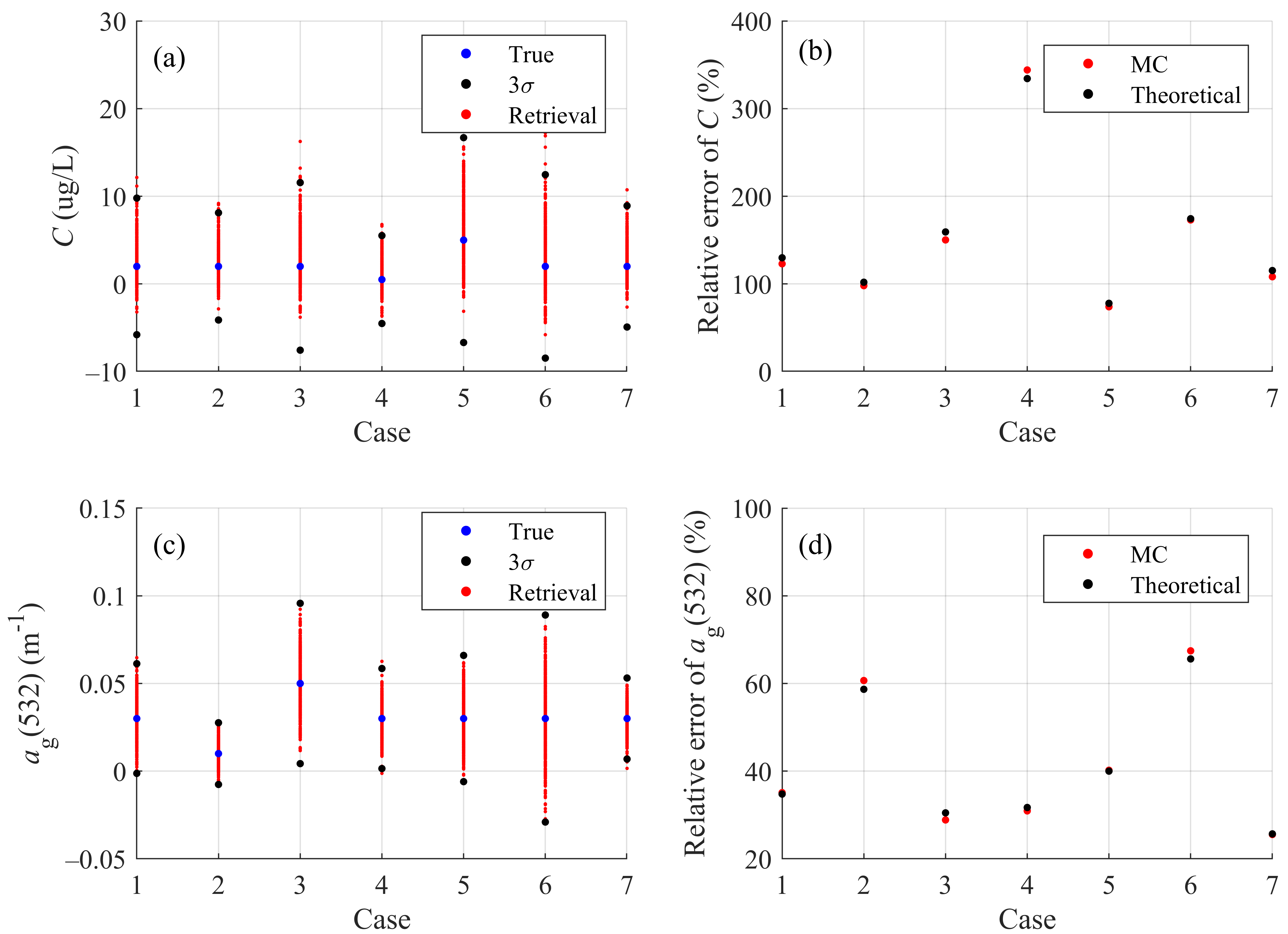
Figure 1. The characteristics of the absorption coefficient in the water: (a) Absorption coefficients of pure seawater [34], Colored Dissolved Organic Matter (CDOM) and particles [27,28,32,35]; (b) total absorption under different C and a g ( λ 0 ) .
Remotesensing 12 03021 g001
Figure 2. C and ag(532) retrieved by the theoretical model and Monte Carlo (MC) method under 7 cases in Table 1. (a) C; (b) relative error of C; (c) ag(532); (d) relative error of ag(532).
Remotesensing 12 03021 g002
Figure 3. Dual-wavelength inversion error under Case 1 in Table 1 of (a) C and (b) ag(532). The black line indicates that the inversion error is 200%.
Remotesensing 12 03021 g003
Figure 4. The effect of λ2 on retrieval error when λ1 is fixed at 532 nm.
Remotesensing 12 03021 g004
Figure 5. Relative errors of chlorophyll (red lines) and CDOM absorption (blue lines) in (a) different ag(532) (Case 1–3 in Table 1); (b) different C (Case 1, 4 and 5 in Table 1); (c) different S (Case 1, 6 and 7 in Table 1).
Remotesensing 12 03021 g005
Figure 6. Relative errors of chlorophyll (red lines) and CDOM absorption (blue lines) in different Δ.
Remotesensing 12 03021 g006
Figure 7. In situ absorption coefficient collected in the Yellow Sea.
Remotesensing 12 03021 g007
Figure 8. Simulated comparison of the retrieval and true results at (a) S1 and (b) S2. Three kinds of retrieval methods are utilized, including (1) dual-wavelengths at 532 and 412 nm, (2) dual-wavelengths at 532 and 440 nm and (3) single wavelength at 532 nm.
Remotesensing 12 03021 g008
Figure 9. Penetration depth probability at (a) 412 nm and (b) 443 nm using the method in [43].
Remotesensing 12 03021 g009
Table 1. Input seawater optical properties in the simulation.
Case1234567
ag(532) (m−1)0.030.010.050.030.030.030.03
C (μg L−1)2.002.002.000.505.002.002.00
S (nm−1)0.0150.0150.0150.0150.0150.0110.019
Table 2. Minimum errors when fixing λ1 and changing λ2 under Case 1 in Table 1.
Retrievalλ1λ2Relative Errors
C412 nm300 nm230.84%
440 nm140.80%
500 nm111.76%
532 nm127.16%
672 nm325.96%
C412 nm358 nm233.66%
440 nm141.42%
500 nm112.06%
532 nm127.62%
672 nm326.10%
ag(532)412 nm300 nm47.64%
440 nm37.58%
502 nm33.64%
532 nm33.60%
672 nm45.98%
ag(532)412 nm358 nm48.08%
440 nm37.46%
502 nm33.38%
532 nm33.52%
672 nm47.28%
Table 3. Inversion error of chlorophyll with single-wavelength lidar under Cases 1–7 and different Δ.
Case1234567
Relative error
(Δ = 10 %)
168.27%66.13%282.32%569.08%79.63%168.27%168.27%
Relative error
(Δ = 20 %)
203.37%102.12%318.17%660.92%100.48%203.37%203.37%
Relative error
(Δ = 30 %)
243.39%142.93%360.77%793.77%126.38%243.39%243.39%

