Comparison of the Sentinel-3A and B SLSTR Tandem Phase Data Using Metrological Principles

Abstract

The Sentinel-3 mission is part of the Copernicus programme space segment and has the objective of making global operational observations of ocean, land and atmospheric parameters with its four on-board sensors. Two Sentinel-3 satellites are currently on orbit, providing near-daily global coverage. Sentinel-3A was launched on 16 February 2016 and Sentinel-3B on 25 April 2018. For the early part of its operation, Sentinel-3B flew in tandem with Sentinel-3A, flying 30 s ahead of its twin mission. This provided a unique opportunity to compare the instruments on the two satellites, and to test the per pixel uncertainty values in a metrologically-robust manner. In this work, we consider the tandem-phase data from the infrared channels of one of the on-board instruments: the Sea and Land Surface Temperature Radiometer, SLSTR. A direct comparison was made of both the Level 1 radiance values and the Level 2 sea surface temperature values derived from those radiances. At Level 1, the distribution of differences between the sensor values were compared to the declared uncertainties for data gridded on to a regular latitude-longitude grid with propagated pixel uncertainties. The results showed good overall radiometric agreement between the two sensors, with mean differences of ∼0.06 K, although there was a scene-temperature dependent difference for the oblique view that was consistent with what was expected from a stray light effect observed pre-flight. We propose a means to correct for this effect based on the tandem data. Level 1 uncertainties were found to be representative of the variance of the data, expect in those channels affected by the stray light effect. The sea surface temperature results show a very small difference between the sensors that could be in part due to the fact that the Sentinel-3A retrieval coefficients were also applied to the Sentinel-3B retrieval because the Sentinel-3B coefficients are not currently available. This will lead to small errors between the S3A and S3B retrievals. The comparison also suggests that the retrieval uncertainties may need updating for two of the retrieval processes that there are extra components of uncertainty related the quality level and the probability of cloud that should be included. Finally, a study of the quality flags assigned to sea surface temperature pixel values provided valuable insight into the origin of those quality levels and highlighted possible uncertainties in the defined quality level.

1. Introduction

The Sentinel-3 (S3) mission contributes to the Copernicus programme space segment, with the objective of making global, long-term observations of atmospheric, ocean and land parameters [1]. There are four main instruments on-board the mission satellites: the Sea and Land Surface Temperature Radiometer (SLSTR), the Ocean and Land Colour Instrument (OLCI); a dual-frequency Synthetic aperture Radar Altimeter (SRAL), and a Microwave Radiometer (MWR). Two S3 satellites are currently on orbit, providing near daily global coverage. Sentinel-3A (S3A) was launched on 16 February 2016 and Sentinel-3B (S3B) on 25 April 2018. Both satellites have a nominal design life of 7.5 years. Two follow-on satellites, models C and D, are in preparation to replace model A and B, so as a whole, the mission is planned to provide 20 years of continuous data.

The SLSTR instrument is primarily designed to retrieve global Surface Temperatures (both Sea (SST) and land (LST)). The specification for the SST retrievals are that they should have an uncertainty of <0.3 K, traceable to international standards and need to continue the 21-year dataset of the Along-Track Scanning Radiometer (ATSR) series [2]. In a similar way to the ATSR sensors, SLSTR scans with two views—measuring both a nadir and a 55${}^{°}$ off-nadir oblique view which provides two atmospheric paths for the same scene, the analysis of which helps mitigate the effect of certain atmospheric components such as stratospheric aerosol. The instrument observes in 11 spectral channels from the visible to the thermal infrared (TIR) (see

Table 1. SLSTR spectral channels.

Channel Name	Centre Wavelength
S1	$0.554$$\mathsf{\mu }$$\mathrm{m}$
S2	$0.659$$\mathsf{\mu }$$\mathrm{m}$
S3	$0.868$$\mathsf{\mu }$$\mathrm{m}$
S4	$1.374$$\mathsf{\mu }$$\mathrm{m}$
S5	$1.613$$\mathsf{\mu }$$\mathrm{m}$
S6	$2.25$$\mathsf{\mu }$$\mathrm{m}$
S7	$3.742$$\mathsf{\mu }$$\mathrm{m}$
S8	$10.85$$\mathsf{\mu }$$\mathrm{m}$
S9	$12.02$$\mathsf{\mu }$$\mathrm{m}$
F1	$3.742$$\mathsf{\mu }$$\mathrm{m}$
F2	$10.85$$\mathsf{\mu }$$\mathrm{m}$

), with TIR channels S7 ( $3.742$ $\mathsf{\mu }$$\mathrm{m}$), S8 ( $10.85$ $\mathsf{\mu }$$\mathrm{m}$) and S9 ( $12.02$ $\mathsf{\mu }$$\mathrm{m}$) used by the SST retrieval [3].

At the launch of S3B, it entered a so-called tandem phase with its twin, S3A. During this initial six-month period of the S3B mission, it flew separated from S3A by just 30 $\mathrm{s}$. This was intended to facilitate a detailed sensor-to-sensor intercomparison to ensure that SLSTR-A and SLSTR-B datasets are well calibrated for the derivation climate data records, before the satellites move to their nominal separated orbits. Such analysis is crucial to build the robust, interoperable data records required for the study of, for example, climatic change. In this study, intercomparisons are performed of the tandem phase data for the S3A and S3B SLSTR instruments (referred to as SLSTR-A and SLSTR-B, respectively), for both the Level 1 (L1) radiometric products and derived Level 2 (L2) SST observations.

In general, such satellite sensor validation activities are capable of monitoring and investigating a wide variety of instrument and retrieval performance characteristics (e.g., [4]). However, a common limitation of such studies is caused by the lack of uncertainty information available for satellite data products. Generally, the outcomes of such comparisons are to compute inter-sensor differences or “biases” in given conditions, but, without uncertainty information, it is difficult to form any definitive quantitative conclusion whether these observed differences indicate the sensors are achieving their specified performance. Efforts are therefore on-going to develop the techniques to facilitate the evaluation and dissemination of satellite sensor uncertainty information [5], with some missions now able to provide this (e.g., Sentinel-2 [6,7]). Sensor uncertainty information is also available for both SLSTR L1 and L2 SST products [3,8].

In this work, the philosophy is to bring metrological principles to Earth Observation data comparison, facilitated by the availability of per-pixel uncertainty components for SLSTR radiometric and SST data products. Crucially within this philosophy, a comparison exercise should be viewed as being primarily aimed at validating uncertainty, as this is ultimately the claimed measurement performance.

In Section 2, the SLSTR tandem data archive is described in more detail, including the available uncertainty information, as well as the methods used for the tandem comparison. Section 3 and Section 4 then provide the radiometric and SST comparison results, respectively. Finally, a discussion of the findings is in Section 5, including describing the advantages of the tandem phase.

2. Materials and Methods

This section details the methodology used to compare SLSTR-A and SLSTR-B within the analysis.

2.1. Tandem Data Archive

The S3A/B tandem phase ran for a period of roughly 6 months and began with an initial drift phase following the launch of S3B, as it moved onto the tandem orbit 30 $\mathrm{s}$ ahead of S3A. The tandem orbit period lasted from 7 June 2018 to 16 October 2018, and was followed by a second drift phase as S3B moved away to its nominal orbit. The final drift phase was divided into two parts, an initial slow drift until 24 October 2018, to facilitate further comparisons during this period increasing of separation, and a final fast drift until S3B reached its nominal orbit on 23 November 2018.

From this full period, a data archive containing the S3A/B products for one full day per week was available for analysis at L1 and smaller subset of this for L2. This was considered sufficient to investigate the full scope of spatial and temporal interest. It should be noted that the tandem phase itself overlapped with initial S3B mission commissioning activities, so the best quality data came from the end of the tandem phase once the instrument had had chance to stabilise.

The SSTs used in this study were derived using the ESA SST retrieval algorithms, which use a set of coefficients derived from modelled brightness temperatures and are a function of path length and total column water vapour taken from a meteorological model [3]. In this study, we have concentrated on the four most common retrievals which are N2 (nadir view only, S8, S9 channels only), N3 (nadir view only, S7, S8, S9 channels), D2 (dual view, S8, S9 channels only) and D3 (dual view, S7, S8, S9 channels). All SST measurements come with flags and quality level estimates based on the GHRSST (Group for High Resolution Sea Surface Temperature) recommendations [9], as well as with an estimate of the likelihood of cloudiness. Uncertainty estimates are also calculated as part of the operational processing and come in two forms: one as the GHRSST Single Sensor Error Statistic (SSES), which has a bias and a standard deviation estimate; and the other as a theoretical uncertainty which is based on trying to propagate different sources of error, including noise and retrieval errors, through to the SST measurement. The SSES and theoretical uncertainty therefore represent two different approaches to SST uncertainty with one based on statistics using observations matched to the drifting buoy network to derive an uncertainty, and the other taking a more metrological approach looking at possible sources of error.

In this study at L1, we focus on the 3 thermal infrared channels used by the SST retrieval. The calibration of these channels is based on the observation of two internal warm blackbody calibration targets that are each viewed once per scan [2]. The data for these channels are provided as brightness temperatures, and come with the information required to evaluate independent (or random) and common (or systematic) components of uncertainty per pixel [10].

2.2. Overview of Methodology

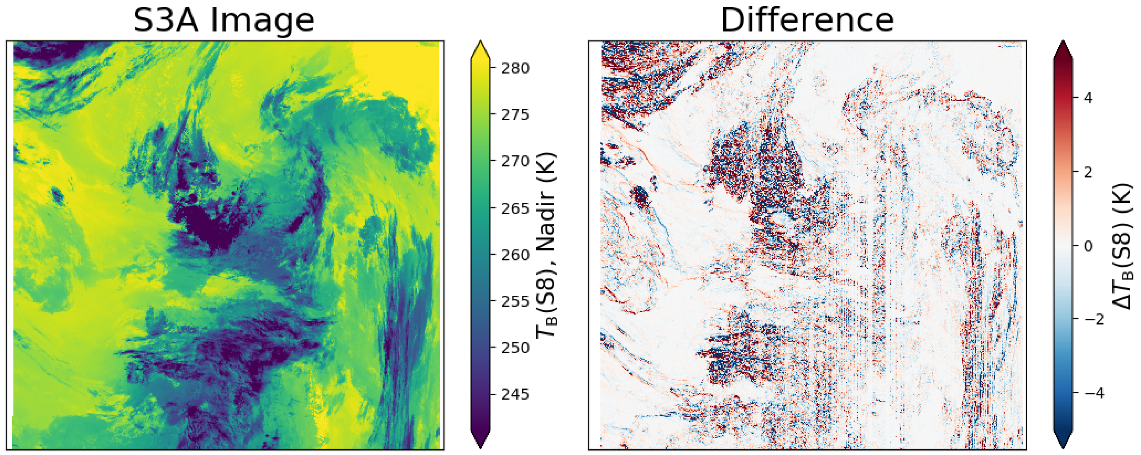
Despite the small time-delay between S3A and B during the tandem phase, pixel-level inter-comparison of co-registered SLSTR-A and B L1 scenes shows that large match-up errors can dominate the observed sensor-to-sensor differences. Such errors are caused by a combination of effects such as geolocation differences, pixel footprint differences, and changes between scenes caused, for example, by cloud movement. These differences affect the L1 data in particular since these scenes are more highly variable than the approximately cloud-free, relatively smoothly varying SST data. An example of this at L1 is shown in Figure 1, where the small radiometric differences found in homogeneous areas are dominated by large differences of up to several kelvin in inhomogeneous areas. The fringing in the difference image is the effect of the nearest-neighbour regridding from the instrument viewing geometry to the image geometry during the L1 ground processing.

For this reason, for the L1 data, comparing a larger region of binned pixels can be preferable, since match-up errors will tend to cancel out. An efficient way to aggregate L1 pixels into larger regions that facilitates a global comparison (enabled by sensors flying in tandem) is to grid the radiometry data onto a regular latitude–longitude grid (often called a Level 3 grid). Match-up errors are further minimised by then filtering for homogeneous grid cells, allowing a more direct comparison of the remaining radiometric biases (described in Section 2.2.2).

L1 products were therefore gridded into $0.5$${}^{°}$ × $0.5$${}^{°}$ grid cells, chosen to balance data volume and match-up error reduction with obtaining a sufficient number of comparison samples to allow statistically robust conclusions across the sensor dynamic range. For the SST data, where we do not expect the same level of spatial variability when compared to the L1 data, the same gridding algorithm was used but on a finer grid of 1 $\mathrm{k}$$\mathrm{m}$ size (the nominal sub-satellite resolution). Furthermore, only pixels with a $30\pm 1$ s time difference between sensors were kept, so, for the SST data, this in general means a single observation only.

2.2.1. Gridding Algorithm and Uncertainty Propagation

To grid the data, the nearest-neighbour method was used, where the value of a given grid cell, ${\langle L\rangle }_{\mathrm{G}}$, is the average of the pixel values, $L_i$, for which it is the nearest grid point, as,

$${\langle L\rangle }_{\mathrm{G}}=\frac{1}{N_{\mathrm{G}}}\sum _{i=1}^{N_{\mathrm{G}}}{L}_i,$$

(1)

where $N_{\mathrm{G}}$ is the number of pixel values contributing to the grid cell. To validate per pixel uncertainties in a comparison of gridded data, the pixel-level uncertainties must be propagated through the gridding process (Equation (1)). This may be achieved following the standard method described in the Guide to the Evaluation of Uncertainty in Measurement (GUM) [11].

For uncertainty propagation, the uncertainty of a given grid cell may be defined with,

$$u^2\left({\langle L\rangle }_{\mathrm{G}}\right)=u_{\mathrm{ind}.}^2\left({\langle L\rangle }_{\mathrm{G}}\right)+u_{\mathrm{com}.}^2\left({\langle L\rangle }_{\mathrm{G}}\right),$$

(2)

where $u_{\mathrm{ind}.}\left({\langle L\rangle }_{\mathrm{G}}\right)$ is the uncertainty due to an error that is uncorrelated (i.e., independent) between grid cells and $u_{\mathrm{com}.}\left({\langle L\rangle }_{\mathrm{G}}\right)$ is the uncertainty due to an error that is fully correlated (i.e., common) between grid cells. This model does not treat error effects that are locally correlated, or structured. This assumption is discussed in more detail below.

Pixel-level error effects that cause the uncertainty $u_{\mathrm{ind}.}\left({\langle L\rangle }_{\mathrm{G}}\right)$, for example instrument noise, may be combined together to give a pixel-level independent uncertainty, $u_{\mathrm{ind}.}\left(L_i\right)$. When pixel-level independent uncertainties are propagated through Equation (1), since independent errors are uncorrelated within $\left\{L_i\right\}$, we obtain,

$$u_{\mathrm{ind}.}^2\left({\langle L\rangle }_{\mathrm{G}}\right)=\frac{1}{N_{\mathrm{G}}^2}\sum _{i=1}^{N_{\mathrm{G}}}{u}_{\mathrm{ind}.}^2\left(L_i\right).$$

(3)

If $u_{\mathrm{ind}.}^2\left(L_i\right)$ is constant for all i, this reduces to $u_{\mathrm{ind}.}^2\left(L_i\right)/N_{\mathrm{G}}$.

Pixel-level error effects that cause the uncertainty $u_{\mathrm{com}.}^2\left({\langle L\rangle }_{\mathrm{G}}\right)$, for example calibration error, may be combined together to give a pixel-level common uncertainty $u_{\mathrm{com}.}^2\left(L_i\right)$. When pixel-level common uncertainties are propagated through Equation (1), since common errors are fully correlated within $\left\{L_i\right\}$, we find,

$$u_{\mathrm{com}.}^2\left({\langle L\rangle }_{\mathrm{G}}\right)={\left[\frac{1}{N_{\mathrm{G}}}\sum _{i=1}^{N_{\mathrm{G}}}{u}_{\mathrm{ind}.}^2\left(L_i\right)\right]}^2.$$

(4)

This is effectively gridding the per pixel common uncertainty and so this does not reduce for increasing $N_{\mathrm{G}}$.

2.2.2. Difference Uncertainty

The comparison of SLSTR-A and B then entails an analysis of the differences between their gridded products, $\Delta {\langle L\rangle }_{\mathrm{G}}$. The uncertainty of a grid cell difference is given by,

$$u^2(\Delta {\langle L\rangle }_{\mathrm{G}})=u^2\left({\langle L_A\rangle }_{\mathrm{G}}\right)+u^2\left({\langle L_B\rangle }_{\mathrm{G}}\right)-2u({\langle L_A\rangle }_{\mathrm{G}},{\langle L_B\rangle }_{\mathrm{G}})+u_{\mathrm{comp}.}^2,$$

(5)

where $u_{\mathrm{comp}.}$ is the comparison uncertainty and $u({\langle L_A\rangle }_{\mathrm{G}},{\langle L_B\rangle }_{\mathrm{G}})$ is the covariance between the SLSTR-A and B gridded values.

The comparison uncertainty, $u_{\mathrm{comp}.}$, is caused by match-up errors that occur on a pixel level. Since these are random from pixel to pixel, the gridding process has the effect of reducing this uncertainty as in Equation (3).

Sensor-to-sensor covariance may be caused by, for example, common calibration errors due to both sensors being calibrated at the same laboratory. Since we are taking the difference of SLSTR-A and B values, a non-zero covariance has the effect of reducing the uncertainty associated with the difference, as errors common to them both should cancel out. No quantitative information, at the time of writing, is available on the covariance between SLSTR-A/B data at L1 or L2, so it is omitted from the uncertainty model, which is a limitation of the following results. In the case of the L1 analysis, this covariance is thought to be relatively small, but, for the SST analysis, the common components are expected to be significant, as the uncertainty is dominated by retrieval effects that are common to both sensors.

Uncertainty Propagation for L1

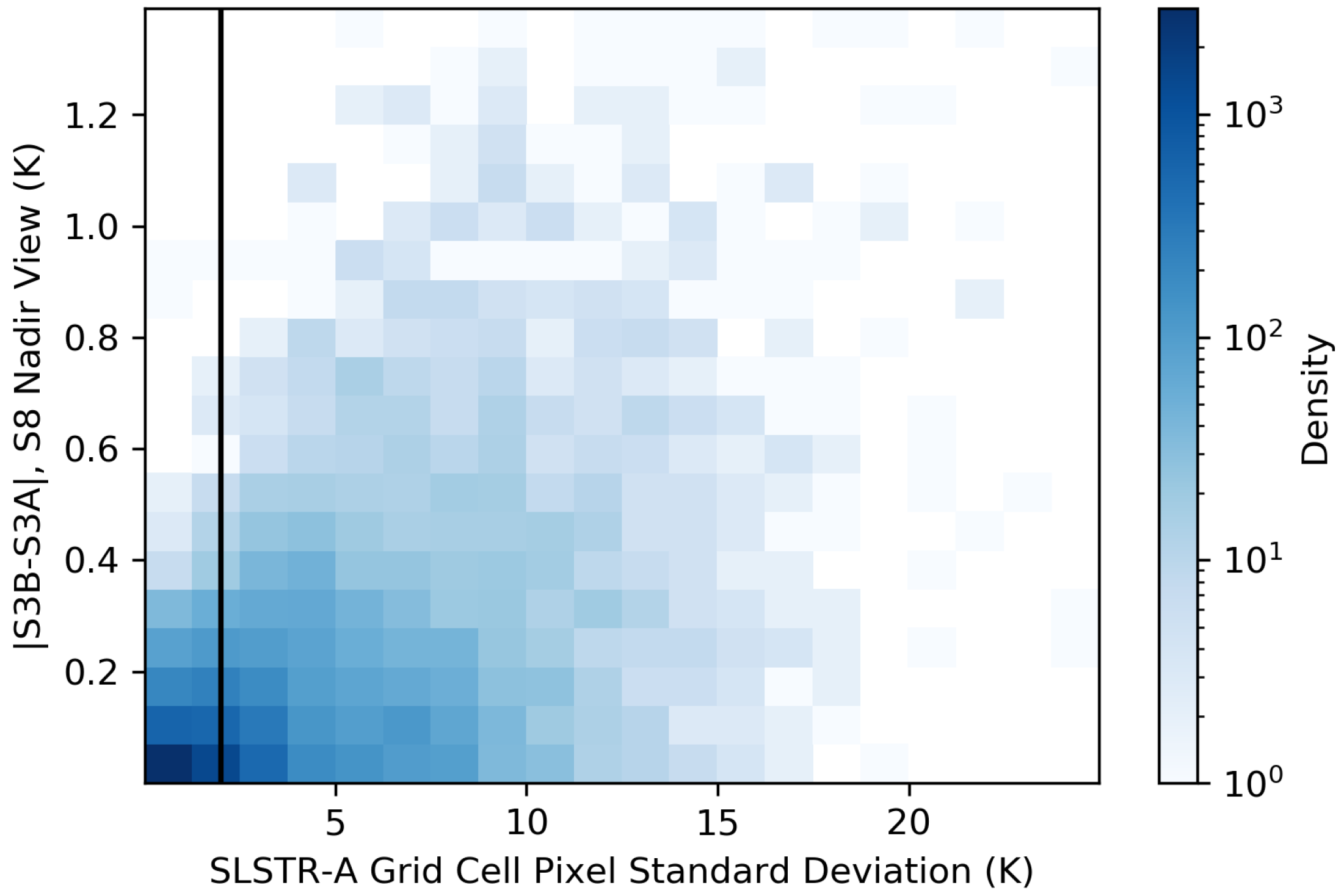
As previously stated, one of the reasons for choosing the L1 grid size was to minimise the impact of random noise and match-up errors. A filtering is then performed to select homogeneous grid cells to further reduce match-up errors. Figure 2 shows the absolute difference between SLSTR-A and B grid cells (S8, nadir view) as a function of the standard deviation of SLSTR-A grid cell pixel values, $\mathrm{std}\left(\left\{L_i\right\}\right)$, for an example orbit of data. The filtering selects pixels where $\mathrm{std}\left(\left\{L_i\right\}\right)<$ 2 $\mathrm{K}$, this is indicated by the black line on the plot. This filtered population of pixels has a standard deviation of SLSTR-A and B differences of ∼$0.2$ $\mathrm{K}$. For SLSTR, typical instrument noise is of the order 30 $\mathrm{m}$$\mathrm{K}$, so random uncertainty in the grid cells differences are therefore driven by the match-up errors.

Since a grid cell of $0.5$${}^{°}$ contains roughly 50 pixels × 50 pixels, random errors are reduced by a factor of 50 compared to their per pixel values (Equation (3)), compared to the common component of uncertainty $u_{\mathrm{com}.}^2\left({\langle L\rangle }_{\mathrm{G}}\right)$ which is of order of $0.05$ $\mathrm{K}$ and does not reduce with averaging, this is small. Thus, we have,

$$u^2(\Delta {\langle L\rangle }_{\mathrm{G}})={\langle u_{\mathrm{cal}.}^2\left(L_{\mathrm{A},i}\right)\rangle }_{\mathrm{G}}^2+{\langle u_{\mathrm{cal}.}^2\left(L_{\mathrm{B},i}\right)\rangle }_{\mathrm{G}}^2,$$

(6)

again noting covariance is omitted. Therefore, a comparison of the gridded products should directly allow the validation of the SLSTR L1 calibration uncertainties.

Not treated here are error effects that are locally correlated, which is not possible as these effects are not described in the available SLSTR uncertainty model [8]. This approximation is assumed reasonable since these locally correlated effects are small (∼1 $\mathrm{m}$$\mathrm{K}$), so handling them separately would not change the evaluated grid cell uncertainty.

Uncertainty Propagation for L2

Since for the finer SST comparison grid resolution, we generally have $N_{\mathrm{G}}=1$, the overall grid cell uncertainty is simply the value of the total pixel-level uncertainty,

$$u^2(\Delta {\langle SST\rangle }_{\mathrm{G}})=u^2\left(SS{T}_{\mathrm{A},i}\right)+u^2\left(SS{T}_{\mathrm{B},i}\right),$$

(7)

again noting covariance is omitted.

2.2.3. Uncertainty-Normalised Differences

The method used to validate these derived uncertainties is based on an analysis of the distribution of SLSTR-A/B differences normalised by the propagated difference uncertainties, i.e.,

$${ϵ}_i=\frac{\Delta {\langle L\rangle }_{\mathrm{G},i}}{u(\Delta {\langle L\rangle }_{\mathrm{G},i})}.$$

(8)

In the case where $u(\Delta {\langle L\rangle }_{\mathrm{G},i})$ represents an uncertainty due to fully uncorrelated error effects within $\{\Delta {\langle L\rangle }_{\mathrm{G},i}\}$, if the variance of differences is well described by its uncertainties, the resulting distribution should be standard normal, i.e., a Gaussian centred on 0 with a standard deviation of 1. Underestimation of uncertainties will lead to an uncertainty-normalised distribution with a standard deviation greater than 1, whereas overestimation of the uncertainties will lead to an uncertainty-normalised distribution with a standard deviation less than 1. As mentioned, particularly at L2, a potentially significant, unquantified covariance between SLSTR-A and B is not included in the estimated difference uncertainty. In this analysis, the effect of this omission would be to cause the uncertainty-normalised difference distribution to narrow, with a standard deviation of less than 1, since the difference uncertainties will be overestimated.

In the case where $u(\Delta {\langle L\rangle }_{\mathrm{G},i})$ represents an uncertainty due to fully correlated error effects within $\{\Delta {\langle L\rangle }_{\mathrm{G},i}\}$, the resulting distribution mean informs if the bias is well described by its uncertainties. If the uncertainty well describes the bias, there is a 68% probability that the uncertainty-normalised distribution mean should be less than 1 and, at a 95% probability, it is less than 2.

3. Results—Radiometric Comparison

The following section gives the results for the comparison of the SLSTR-A/B tandem phase L1 data, including: overall radiometric differences, uncertainty validation and key sensitivity analyses—in particular, scene temperature dependence and temporal stability of the comparison.

3.1. Overall Radiometric Differences

To summarise the average radiometric differences between SLSTR-A and B, we considered a single orbit of night-side gridded data. The selected orbit is from 3 September 2018, a day late on in the tandem phase such that SLSTR-B had stabilised following the initial commissioning activities.

The comparison is restricted to pixel values in the nominally linear region of the instruments’ dynamic ranges, defined here as measured temperatures greater than 250 $\mathrm{K}$. The location of this linear region is largely governed by the set-point temperatures of the instruments’ hot and cold blackbody calibration targets, which are held at ∼303 $\mathrm{K}$ and ∼265 $\mathrm{K}$, respectively. Temperatures close to, and especially between, these points are the effective dynamic range of the sensor, so chosen to optimise performance at sea surface temperatures ($\gtrsim$$-2{}^{°}\mathrm{C}$. Outside of this range measurement uncertainties increase considerably, particular for colder temperatures where the Earth radiance is very low, especially for the S7 channel $\left(3.742\mathsf{\mu }\mathrm{m}\right)$. An analysis of the sensitivity of the differences as a function of scene temperature is given in Section 3.3.

The results of the comparison, given in

Table 2. Mean and standard deviation of differences between SLSTR-A and B observations ($\mathrm{S}3\mathrm{B}-\mathrm{S}3\mathrm{A}$), in the linear detector region (data: 3 September 2018).

Channel Name and View	Mean Difference/K	Standard Deviation/K
S7 Oblique	0.06	0.13
S8 Oblique	−0.01	0.11
S9 Oblique	−0.05	0.11
S7 Nadir	0.06	0.10
S8 Nadir	0.01	0.06
S9 Nadir	−0.04	0.06

, show small mean differences for channels S7, S8 and S9 in both the nadir and oblique views, of order 10 $\mathrm{m}$$\mathrm{K}$, with slightly lower standard deviation of differences in the nadir view, particularly for channels S8 and S9.

3.2. Uncertainty Validation

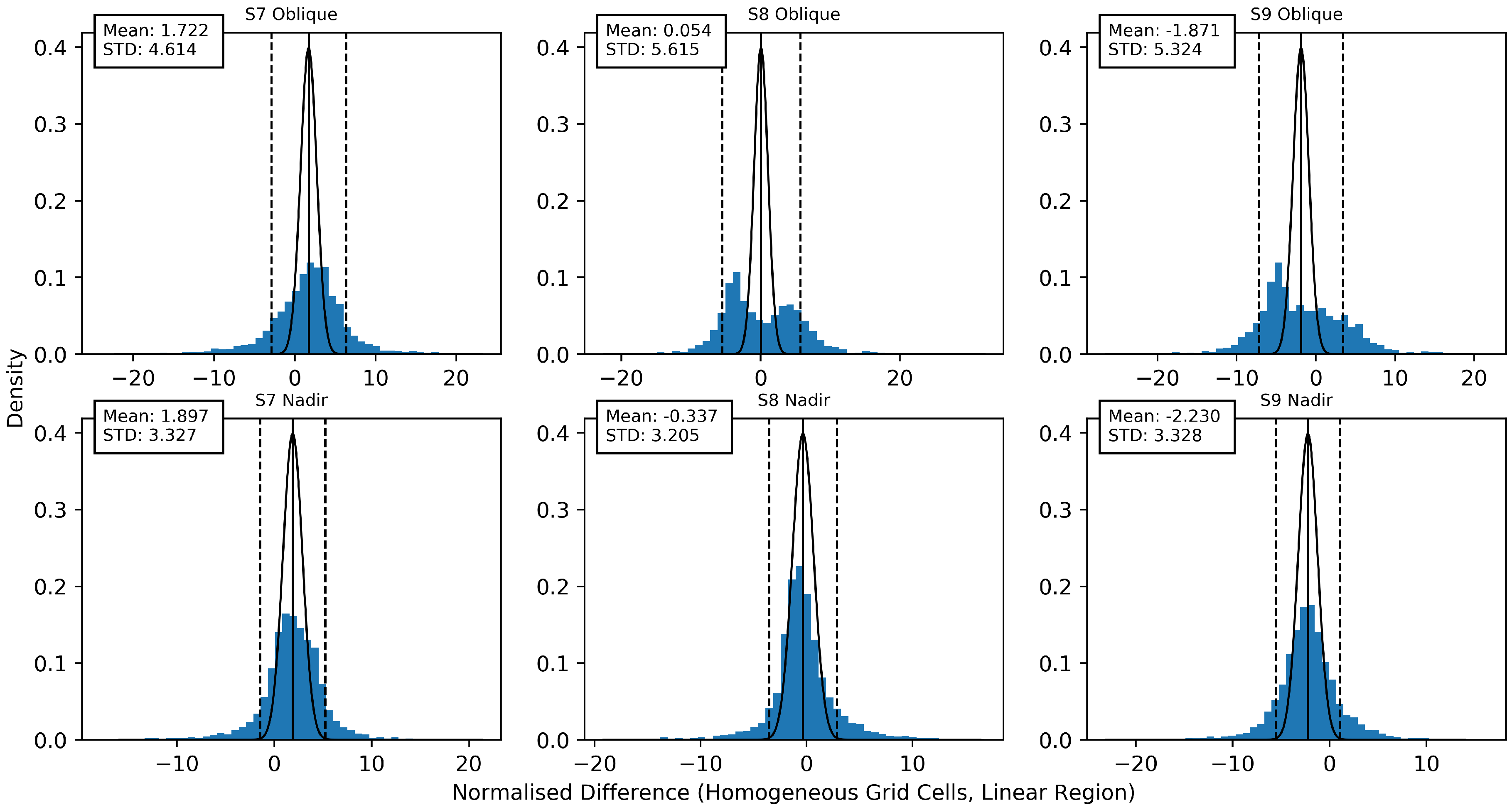
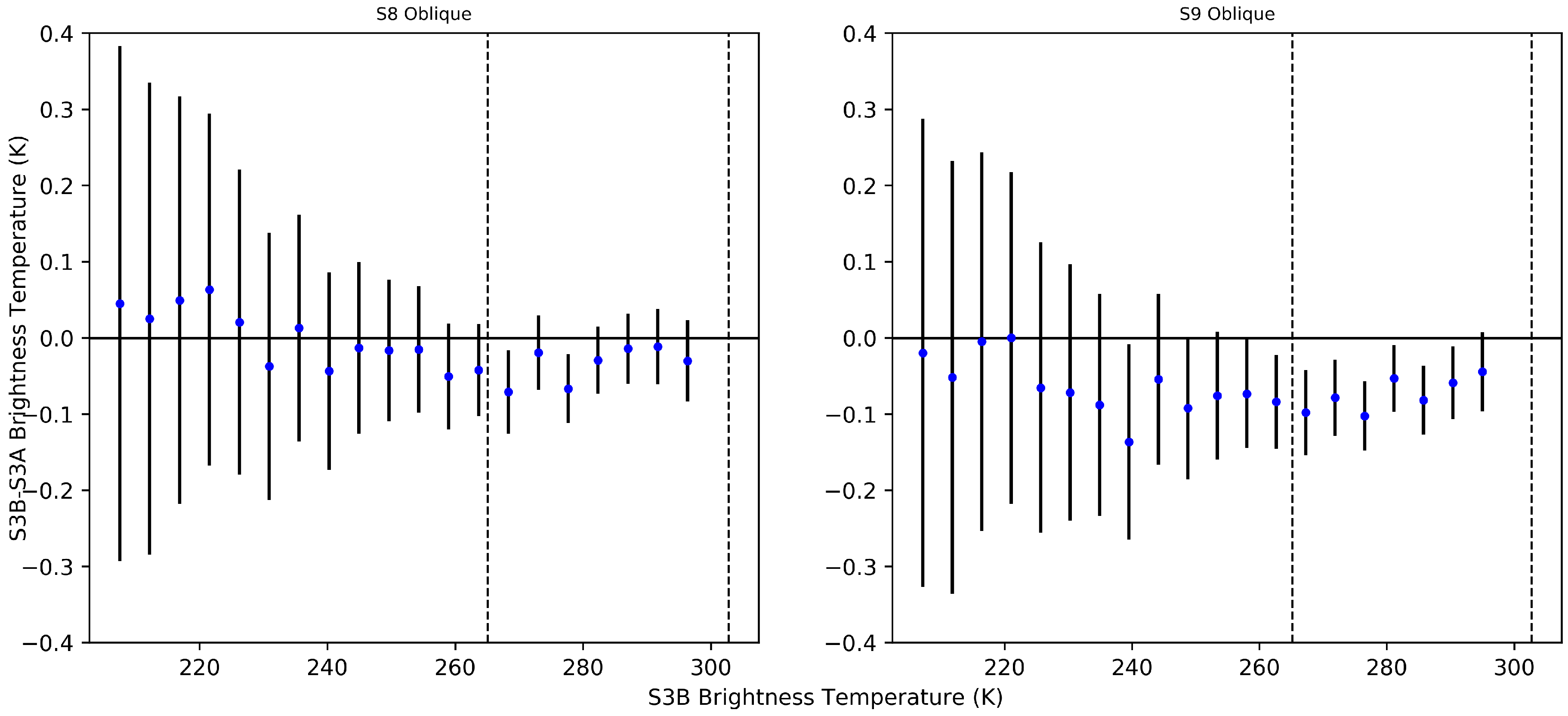
For the data analysed in Section 3.1, the uncertainty validation methodology described in Section 2.2.2 was applied. The resulting plots of uncertainty-normalised SLSTR-A/B differences for channels S7, S8 and S9 in nadir and oblique views are shown in Figure 3. Within the context of the metrology-based approach this study takes, uncertainty validation provides the key result of the comparison exercise, quantitatively determining if the sensors are meeting their expected performance.

Since the uncertainty that the data are normalised by is due to calibration errors that are fully correlated within the measurements, the distribution mean, $\mu$, is the metric of interest. The width of the distribution is caused by unquantified uncertainty due to random errors, for example, remaining match-up errors.

As found in the analysis of radiometric differences, the nadir channels appear to perform best. In particular, the S8 nadir channel is performing well, where for the uncertainty-normalised distribution $\left|\mu \right|<1$, validating the claimed uncertainty this channel. The S9 nadir performs somewhat worse, where $\left|\mu \right|>2$, indicating the calibration uncertainty for this channel is likely too small. For the S7 channel in both the nadir and oblique view, we find $\left|\mu \right|<2$ indicating the calibration uncertainties seem reasonable given the observed bias.

For channels S8 and S9 in the oblique view, however, we find non-normal distributions that point to a more significant issue. This indicates there is a significant error effect missing from the radiometric uncertainty budget for these channels, demonstrating the need for either some sort of correction or an update to the uncertainty budget. This is discussed further in Section 3.3, where a potential correction is investigated.

Figure 3 shows that, in general, the calibration uncertainties for SLSTR TIR channels are likely somewhat underestimated. This is especially the case since any covariance between SLSTR-A and B (omitted from this uncertainty budget) would tend to reduce the difference uncertainties, which the existing uncertainties would have to further compensate for.

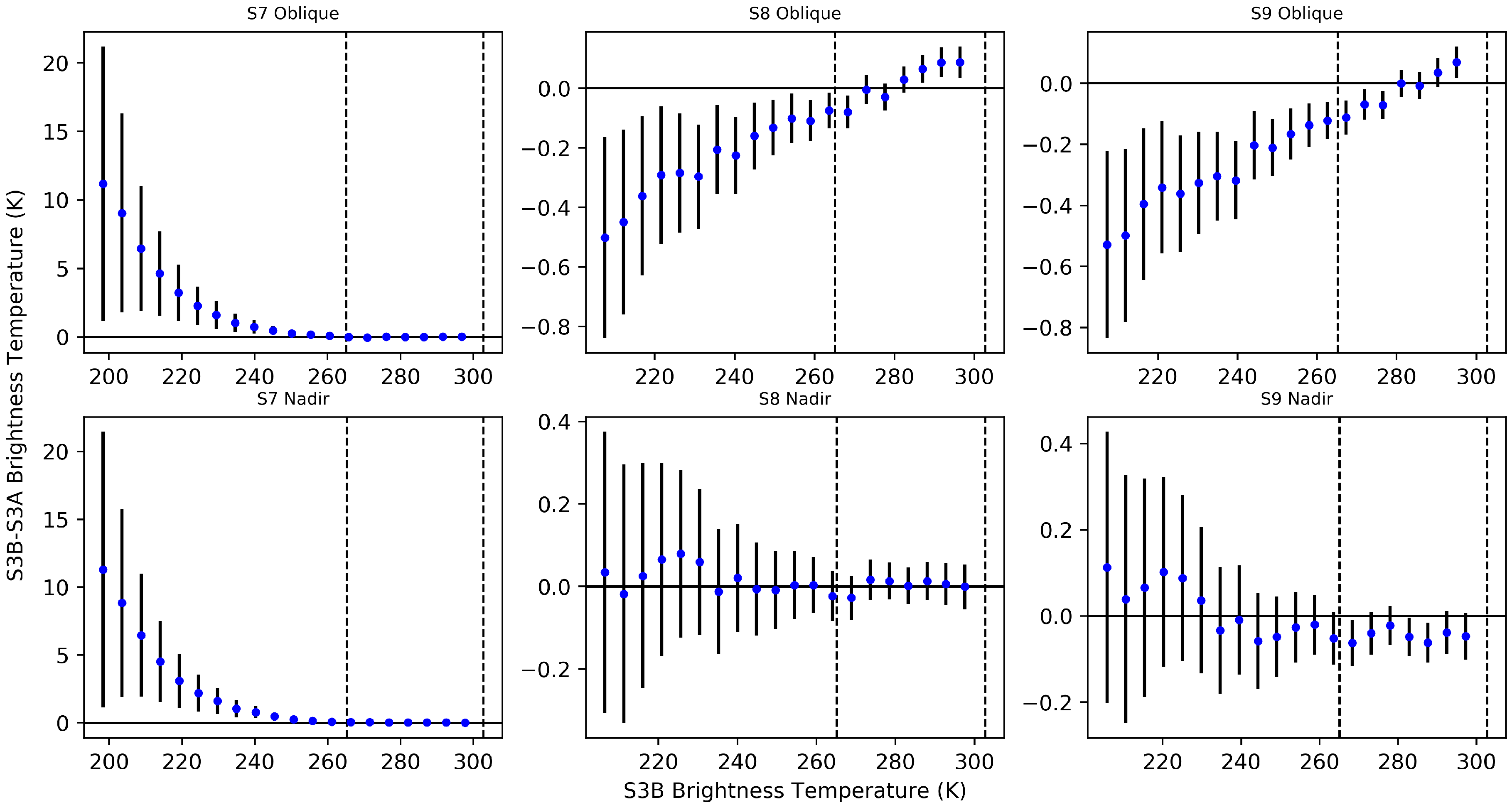
3.3. Sensor Linearity

The linearity of the sensors, may be examined by plotting their differences as a function of scene temperature. This gives an insight into the performance and validity of the instrument measurement function, as artefacts of poorly characterised and formulated measurement function will be present in functional form of the comparison results. Figure 4 shows the linearity of the grid cell difference data examined in Section 3.1. Here, the SLSTR-A/B differences have been binned into evenly-spaced brightness temperature bins, with uncertainties propagated following the the same approach as for spatial binning described in Section 2.2.1.

The uncertainties shown in Figure 4 are displayed as “expanded uncertainties” [11]—in this case with a coverage factor, k, of 3 (often called 3 $\sigma$). If the uncertainties are valid, there is therefore a ∼99.7% probability that the observed difference is covered by these uncertainties (i.e., the uncertainty bar crosses 0). As expected from the results in the previous section, the plots show this is the case for only some channels/views within the linear region of the detectors. Again, the linear region of instrument response, as explained in Section 3.1, is defined as scene temperatures close to those of the two blackbody calibration targets (roughly >250 $\mathrm{K}$). These blackbody temperatures are plotted as dashed lines in Figure 4 for reference, which define the linear region of detector response.

The best performing channels are again in the nadir view, especially for S8, which shows reasonable consistency all the way to lower end of the scene temperature range. For S9, a small offset (∼50 $\mathrm{m}$$\mathrm{K}$) is observed between SLSTR-A and B, which generally exceeds a level justified by the uncertainties, as observed in Section 3.2. One potential cause for this could be detector spectral response sensitivity to temperature, as this is not compensated for in the SLSTR measurement function. This is recommended for future analysis.

S7 performs similarly in both nadir and oblique views, with reasonable agreement found in the linear region that severely degrades at colder scene temperatures. As previously remarked, signal at these temperatures is extremely low in this $3.742$ $\mathsf{\mu }$$\mathrm{m}$ channel, but the large differences are not explained by the large uncertainties. Additionally, the differences vary very smoothly as a function of decreasing temperature and so there is scope in future work to model this to, for example, harmonise the calibration of the two SLSTR sensors.

Again, poor performance is found for the S8 and S9 channels in the oblique view. For these channels, an offset that trends across the scene temperature range is found, explaining the non-normal distributions found in Figure 3. Such a result indicates there is an error effect in one or both of the instruments that should be corrected for, or an additional component should be added to the uncertainty budget. Such an effect has, in fact, been observed since the pre-flight calibration in both instruments, though primarily SLSTR-A, in channels S8 and S9 in the oblique view [10] and is thought to be the result of an internal stray light effect caused by a non-black coating of an optical stop within the instrument that was modified for SLSTR-B.

An empirical correction was proposed for this effect; however, although it is clearly seen in the tandem analysis, initial comparisons between SLSTR-A and IASI-A could not observe this effect on-orbit and so no correction was applied at the time [12].

Here, we now propose to apply the correction originally defined in [10] to both SLSTR-A and B data, $\Delta L$, as

$$\Delta L=X\Delta L_{\mathrm{BB}1}-(1-X)\Delta L_{\mathrm{BB}2},$$

(9)

where X is

$$X=\frac{C_{\mathrm{E}}-C_{\mathrm{BB}2}}{C_{\mathrm{BB}1}-C_{\mathrm{BB}2}},$$

(10)

with $C_{\mathrm{E}}$, $C_{\mathrm{BB}1}$, and $C_{\mathrm{BB}2}$ the observed counts from the Earth and black body calibration targets, respectively. Finally,

$$\Delta L_{\mathrm{BB}1/\mathrm{BB}2}=g\left[L\left(T_{\mathrm{Stray}}\right)-L\left(T_{\mathrm{BB}1/\mathrm{BB}2}\right)\right],$$

(11)

where g and $L\left(T_{\mathrm{Stray}}\right)$ are the model parameters to be optimised.

The result of fitting and applying this correction to both SLSTR-A and B based on the tandem dataset are shown in Figure 5. A significant overall improvement in the agreement between SLSTR-A and B is found, removing the strong trending bias in the uncorrected data. However, the performance is still worse than the equivalent channels in the nadir view, particularly in the S9 channel. Further investigation is required before any recommendation could be made for implementation, to test the performance of the correction.

3.4. Temporal Stability

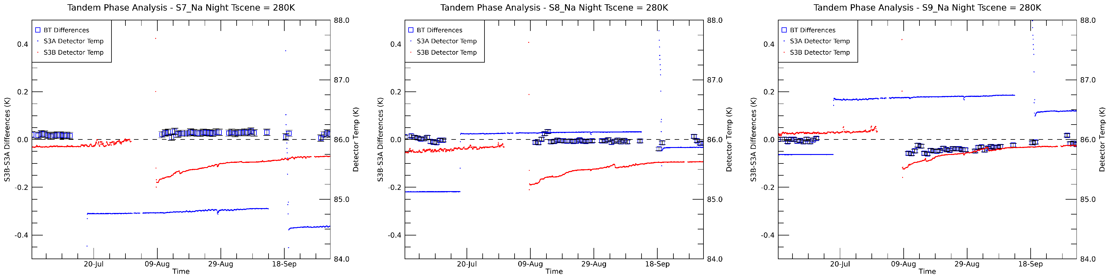
Finally, an analysis of the temporal stability of SLSTR-A/B during the tandem phase was performed by monitoring changes in the sensor-to-sensor differences in days of gridded data during the tandem phase, as shown in Figure 6 for night-time observations of 280 $\mathrm{K}$ scene temperatures.

The most obvious feature during this period is a step change in the observed differences apparent from August onwards. This step change is likely to be caused by two scheduled mission activities that took place shortly before this. Firstly, a planned change in the set-point temperature of the SLSTR-A detectors occurred in July; this was followed by outgassing of SLSTR-B shortly after. The resultant temperature change for both sensors is shown as solid lines in Figure 6 for reference. The spectral response functions (SRFs) of SLSTR TIR channels have been shown to be temperature sensitive [10], and so the change in the radiometric response is likely to be linked to the change in instrument temperature. Temperature sensitivity as the source of step change is further supported by the fact that channel S9 is the most temperature sensitive channel and shows the largest step change. After this initial step change, the channels S7 and S8 seem to stabilise fairly quickly, whereas S9 differences drift by almost 0.1 K as the temperature of SLSTR-B levels off.

4. Results—Sea Surface Temperature Comparison

Only a limited amount of data was made available for the SST analysis with SLSTR-A and SLSTR-B data provided for certain days in September and December 2018. September was when the closest approach occurred so we have concentrated on the three available days of data (3, 10 and 24 September 2018, respectively). September 17 was not used due to a processing error which led to all SLSTR-A SST data being flagged as bad.

Each SST observation comes with a set of flags which provide information related to quality and status [9] as well as algorithm type (N2, N3, D2, D3) and the probability of cloud. In this analysis, only quality flags 3 to 5 for ocean pixels have been considered.

4.1. Quality Level 5 (Best) SSTs

The differences in SST between SLSTR-A and SLSTR-B for all valid pixels of excellent quality (GHRSST quality level of 5) for the September data are closely matched with a mean bias of $-0.014$ $\mathrm{K}$ and a standard deviation of $0.119$ $\mathrm{K}$. Figure 7 shows the differences separated out by retrieval algorithm (N2, N3, D2 and D3) and small differences between them can be seen at the sub 0.1 K level (see

Table 3. Mean and standard deviations ($\sigma$) for different quality levels and algorithms for the SST differences. The “All” case on the first line means all algorithm retrievals are combined together to give a single set of statistics.

Algorithm	Quality Level 3		Quality Level 4		Quality Level 5
	Mean/K	$\mathit{\sigma }$/K	Mean/K	$\mathit{\sigma }$/K	Mean/K	$\mathit{\sigma }$/K
All	−0.18	0.18	−0.093	0.13	0.014	0.119
N2	−0.23	0.16	−0.12	0.12	−0.076	0.082
N3	−0.03	0.17	−0.03	0.12	−0.043	0.096
D2	0.06	0.13	0.05	0.14	0.074	0.100
D3	−0.01	0.24	−0.06	0.14	0.031	0.130

). In part, these small differences are likely due to the use of incorrect retrieval coefficients for S3B, where currently the S3A coefficients are being used for S3B data, as the S3B specific coefficients are yet to be derived and applied within the operational SLSTR processing. Any bias caused by the missing SST coefficients can be reduced further by applying the SSES bias term (see below).

The fact that such small differences in the data are observable using the tandem data does, however, highlight the level of detail it is possible to attain. Because of the issue with the current SLSTR-B SST retrieval coefficients, however, care must be taken in interpreting the data as some of the variance will, in part, be due to using incorrect retrieval coefficients rather than showing true differences between the sensors and/or the errors caused by small timing/geolocation differences. Once the SLSTR-B retrieval coefficients have been properly calculated, the tandem data will need to be reassessed so the current work must be considered to be very preliminary.

4.2. SST Differences at Different Quality Levels

SST data are available for a range of quality levels defined in

Table 4. Criteria for different quality levels defined for SLSTR (based on private communication, Claire Henocq, ACRI) and range of $P_{\mathrm{Clear}}$ per quality level in data.

Quality Level	QL Comment	${\mathit{P}}_{\mathbf{Cloudy}}$ Threshold	Additional Factors
0	No data	<0	No data
1	Cloud contaminated data	>0.5	$SST<SS{T}_{\min }$ and/or missing meteorology data
2	Worst quality of usable data	>0.2	Zenith Angle > 55${}^{°}$
3	Low quality of usable data	0.1–0.2	Twilight, inland water
4	Acceptable quality of usable data	<0.1	Aerosol detected
5	Best quality of usable data	"

. Here, we have concentrated on data with quality level 3 to quality level 5 while noting that the current recommendation is that only quality level 5 (best quality) data should be used for accurate analyses. Table 3 shows the statistics for all algorithms/quality levels and shows a similar pattern to the quality level 5 plots in that there are algorithm dependent biases/standard deviations of varying sizes. In particular, the N2 retrieval has an increasingly large bias for quality levels 3 and 4 compared to the other retrieval algorithms. Lastly, as the quality level decreases (from 5 to 3), the standard deviations show an increase for all retrieval algorithms which indicates that there is likely to be a missing uncertainty component related to the quality level itself.

We also note that the SLSTR-B GHRSST data includes an SSES bias term which is designed to correct for some of the retrieval coefficient errors.

Table 5. GHRSST SST bias values for SLSTR-A and SLSTR-B for quality levels 3, 4 and 5.

Algorithm	Quality Level 3		Quality Level 4		Quality Level 5
	SLSTR-A	SLSTR-B	SLSTR-A	SLSTR-B	SLSTR-A	SLSTR-B
N2	−0.3	−0.15	0.24	0.34	−0.01	0.01
N3	0.0	−0.07	0.06	0.00	0.04	0.06
D2	0.15	−0.07	−0.5	−0.18	0.02	−0.05
D3	0.12	0.07	0.39	−0.13	0.00	0.01

shows the SLSTR-A/SLSTR-B SSES bias terms. In the data provided, there was no difference in the bias values between SLSTR-A and SLSTR-B because the data were taken during commissioning where no updated estimates of the SLSTR-B retrieval coefficients or of the SSES values were available. The SLSTR-B values shown in Table 5 are therefore taken from a file taken on 2 July 2019 when SLSTR-B SSES values were available. It should also be understood that the SSES values for quality levels 3 and 4 are not well determined due to a lack of matchup data and that the recommendation is that they should only be trusted for quality level 5 data.

Applying the SSES bias values to the mean values from the Tandem data (Table 3) would then give SSES bias corrected means for quality level 5 pixels differences of N2: $-0.056$, N3: $-0.023$, D2: $-0.03$ and D3: $-0.041$ which are, apart form the D3 case, closer to a zero difference than was the case for uncorrected values. It can also be seen, however, that the SSES bias will not improve most of the means for the lower quality levels, reinforcing the recommendation not to use them for quality levels 3 and 4.

One last point to make about the SSES bias term is that there can be significant differences in the bias between quality levels. As we will show below, the Tandem data have cases where the quality level itself changes between SLSTR-A and SLSTR-B observations so the application of the SSES bias term to the data would then lead to spurious jumps in the values. For this reason, and the reason that the SSES bias terms are not applicable for quality levels 3 and 4, we have not applied the GHRSST SSES bias to any of the subsequent Tandem analysis to retain a systematic approach across all quality levels.

4.3. Changes in SST Quality Levels

While the previous sections have shown the SST differences between SLSTR-A and SLSTR-B for different quality levels, there are also cases where at the same location the quality level changes between the SLSTR-A and SLSTR-B observations.

Table 6. Fraction of pixels with a 30 s time difference in different quality levels for SLSTR-A and SLSTR-B.

QL SLSTR-A & SLSTR-B	Number of Matches	Fraction of Total
5 & 5	47,135,591	76.1%
4 & 4	7,575,917	12.2%
3 & 3	3,684,585	6.0%
5 & 4	1,472,581	2.4%
5 & 3	1,654,688	2.7%
4 & 3	421,671	0.7%

shows the number of cases for the different SLSTR-A and SLSTR-B quality level combinations where we have limited it to cases where the quality level has to be greater than or equal to 3. Most pixels have a quality level of 5 for both SLSTR-A and SLSTR-B and overall 94% of pixels have the same quality level. Six percent of pixels, however, change their quality level after 30 s. Uniquely, the tandem data allow us to try and see why, in part, the quality level can change within such a short time interval.

A change in quality level can be caused by a number of processes. Most obviously, there may be a change in the local conditions (such as the close proximity of cloud), but the impact of noise on the cloud/aerosol detection probability can also change the quality level.

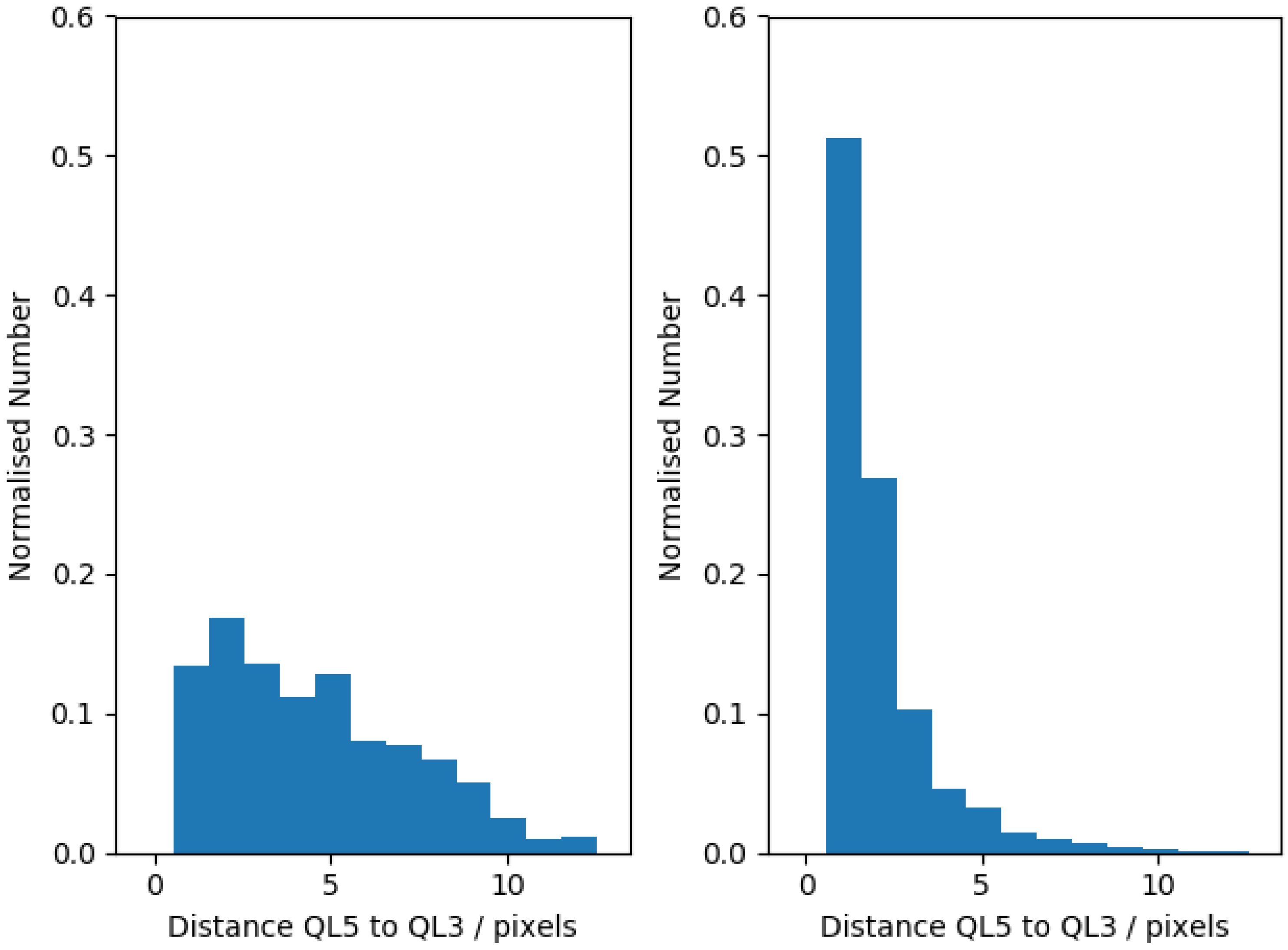
To investigate the impact of nearby clouds, we can look at the location of the nearest SLSTR-A pixel which has the same quality level as the SLSTR-B pixel. Figure 8 shows two plots. The left-hand plot shows the distribution of the distance in pixels of the nearest quality level 3 pixel when both SLSTR-A and SLSTR-B are at a quality level of 5. This can be considered to be analogous to the background distribution. The right-hand plot shows the distribution of the nearest quality level 3 pixel when the SLSTR-B observation has changed the quality level to a value of 3 from an SLSTR-A quality level of 5. Compared with the background distribution, this distribution is much more peaked to smaller distances implying that the change in quality level is due to the proximity of lower quality (likely cloudy) pixels. Figure 8 shows that approximately 80% of the cases where the quality level changes may be caused by the proximity of a lower quality level pixel and 20% may be due to observational uncertainty.

What does a change in quality level in 30 s mean? Clearly, the nearby presence of lower quality pixels indicates that the SST quality level may be subject to rapid change over time and thus is not stable. Of course, this does not impact the quality level derived from the instantaneous measurement but may change the interpretation of cloud mask/quality level assignment schemes which use cloud proximity as one of the tests. This variability may also impact uncertainty components related to SST averaging such as those described in [13].

There is also a population of pixels where the distance to the lower quality level pixel is large. In this case, it is likely that the change in quality level is driven more by measurement uncertainty. This then means that there is a form of uncertainty in the quality level assignment itself. To date, no consideration of an uncertainty on the quality level assignment within SST datasets has been made.

4.4. SST Differences When Quality Level Changes

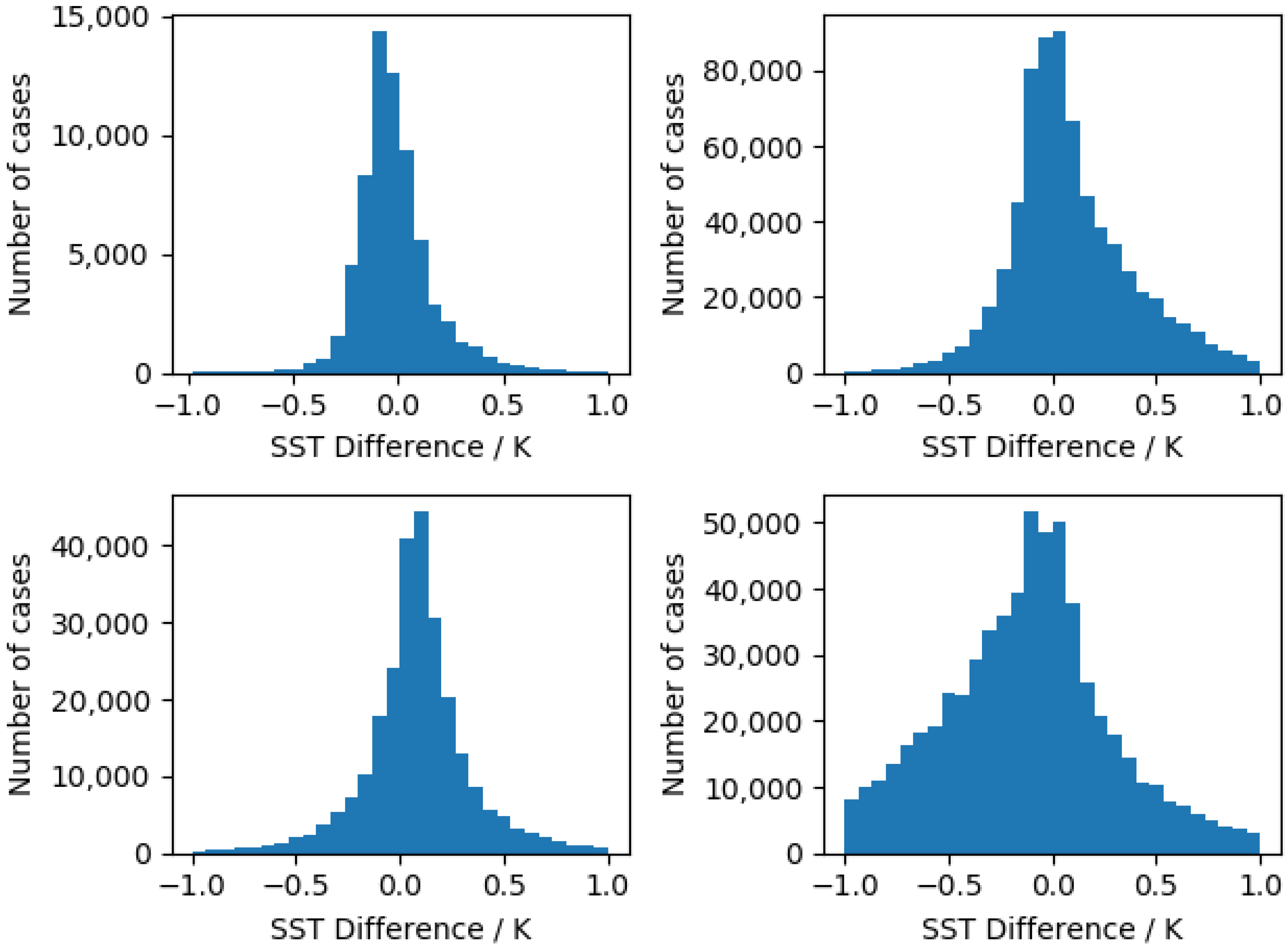
Figure 9 shows the SST differences where SLSTR-A uses quality level 5 pixels and SLSTR-B uses quality level 3 pixels for all algorithm types and shows small mean differences (less than or of order $0.1$ $\mathrm{K}$) together with distinct non-Gaussian behaviour with extended tails with, for example, the D3 differences being very large. This implies that there is an extra source of error between the two quality levels which may be related to the presence of higher probability of cloud. This will be looked at in the next section.

4.5. SST Difference and Cloud Probability

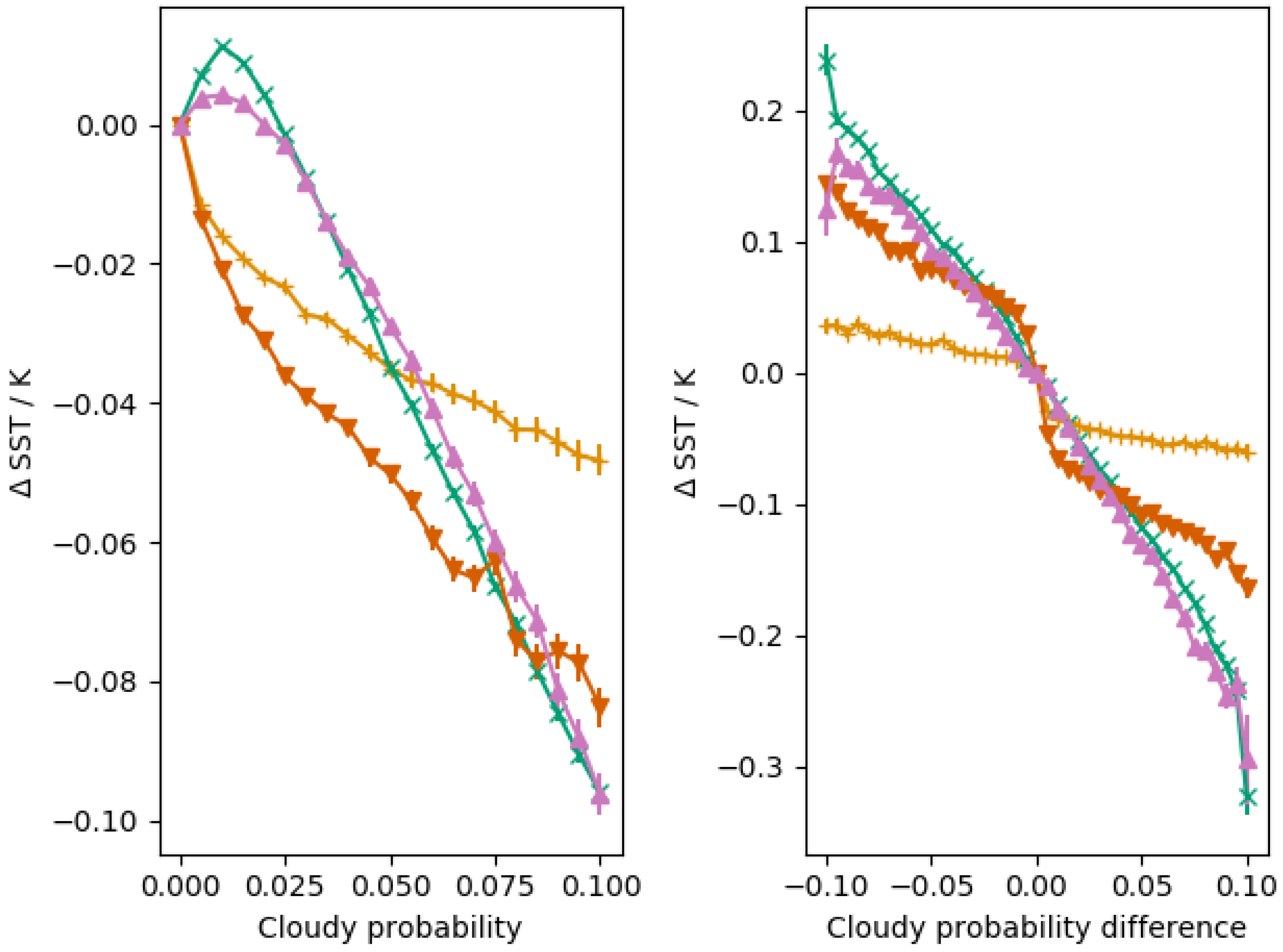
The right-hand panel of Figure 10 shows trends in all algorithms (N2—blue, N3—Orange, D2—Green, D3—Red) as a function of cloud probability (defined as the probability of cloud for the nadir view only) for quality level 5 where any bias at zero cloud probability has been removed. All retrieval algorithms show a small increasing negative bias a function of increasing SLSTR-A nadir cloud probability. We can also look at the SST difference as a function of the difference in the probability of cloud between SLSTR-A and SLSTR-B (right-hand plot) which will reflect real differences in the observed scene and shows that the SST is colder when one sensor has a higher cloud probability. While this may seem obvious, the tandem data are now allowing this trend to be parameterised and modelled. Looking more closely, it also looks like the two channel algorithms (N2—Blue, D2—Green) have a slightly different behaviour to the three channel algorithms and the N2 algorithm is again an outlier.

4.6. SST Uncertainties

Along with the SSTs, the SLSTR L2 data come with two forms of uncertainty. The first is the GHRSST uncertainty parameterized in the SSES (Single Sensor Error Statistic) standard deviation. For each algorithm and quality level, there is a single value which provides a very coarse estimate of what the SST uncertainty really is. In addition, included with the SLSTR L2 is an estimate of a theoretical uncertainty based on a combination of instrumental (L1) uncertainty terms (of order 0.05 K see Figure 4) as well as other, more systematic terms related to possible retrieval biases such as the pseudo-random uncertainty (of order 0.07 K, [3]).

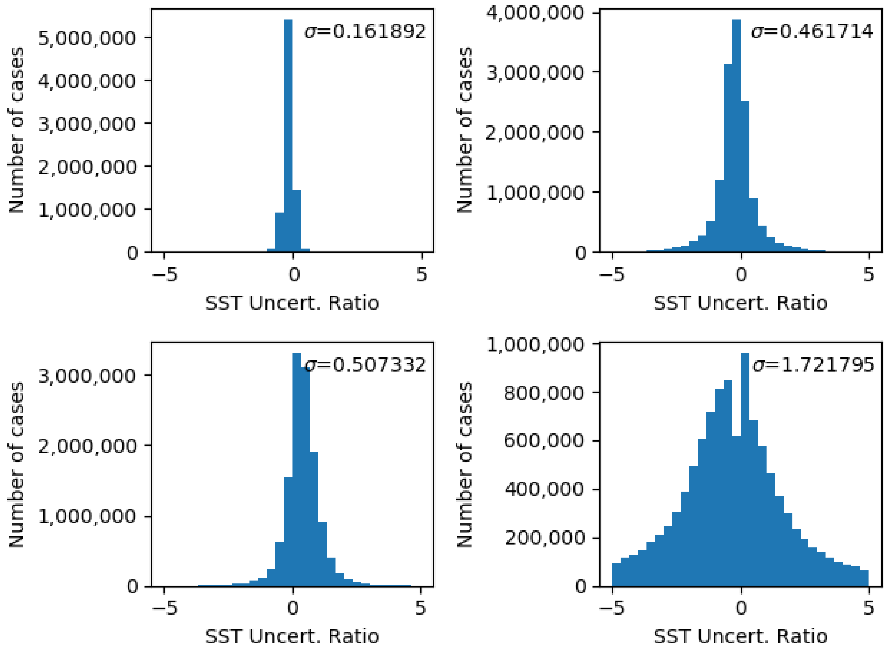
Figure 11 compares the SSES values to the theoretical uncertainties and shows that there are distinct differences between the SSES value per algorithm and the theoretical estimates. For N3/D2, it looks like there may be some small, missing components to the theoretical uncertainty budget, but for N2 and D3 the difference is far larger. For N2, the uncertainty-normalised distribution standard deviation looks like the retrieval is significantly over estimating the theoretical uncertainty, while for D3 the uncertainties look to be significantly underestimated. Of course, the SSES values are themselves uncertain due to to representivity issues (including spatial errors, time errors and geolocation errors).

For the purpose of this study, we have concentrated on the theoretical uncertainties primarily because they more closely approximate a metrologically based uncertainty. However, it must be remembered that the systematic components of SST uncertainty that are covariant between SLSTR-A and B are likely to be much larger than was the case for the L1 analysis so the uncertainty-normalised distribution standard deviation should be less than 1. In fact, we expect the standard deviation to be closer to 0.5 given the relative size of the random and systematic components included in the uncertainty model (see above). 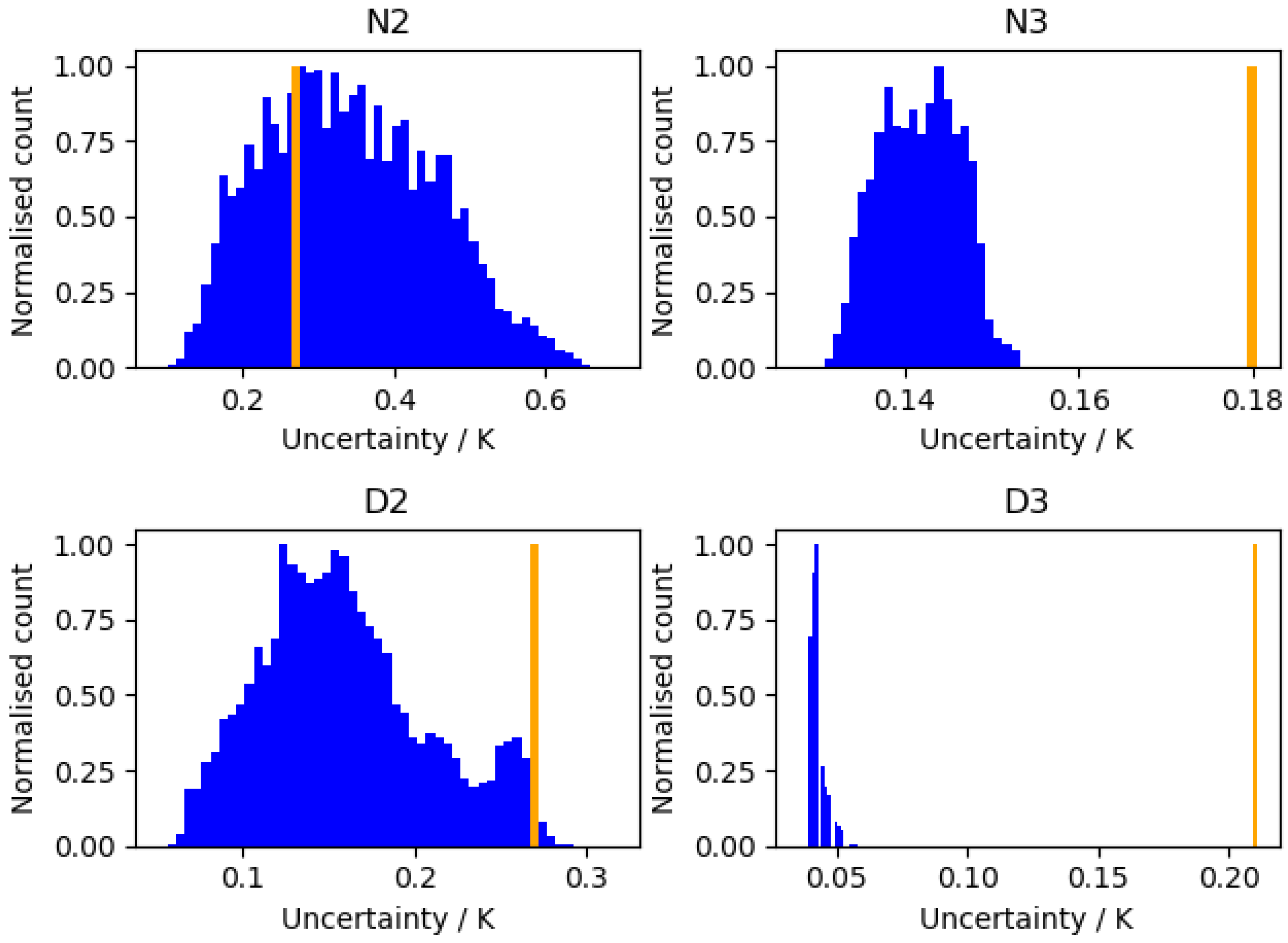Figure 12 shows the uncertainty-normalised distribution for each algorithm and indicates again that the theoretical uncertainty will need revision. As discussed previously, comparing the SSES to the N2 theoretical uncertainties implied that many were overestimates relative to the SSES values, whereas the D3 theoretical uncertainties seem to be significantly underestimated. We note that, from [3], the N2 theoretical uncertainty model for the pseudo-random component includes a $\sec \left(\theta \right)$ term based on an AATSR model which is not included for the other retrievals. Given that SLSTR has a much wider swath than the AATSR, the use of an AATSR based model may be causing issues with the SLSTR N2 uncertainty model. For D3, it looks like there are significant missing uncertainty components the origin of which will need to be further investigated. In the case of the N3 and D2 retrievals, the uncertainty-normalised distribution width is more in line with the expectations assuming the values of the random and systematic uncertainties quoted above.

Looking at the other quality levels,

Table 7. Standard deviations ($\sigma$) of the uncertainty-normalised distributions for different quality levels and algorithms.

Algorithm	Quality Level 3	Quality Level 4	Quality Level 5
	$\mathit{\sigma }$/K	$\mathit{\sigma }$/K	$\mathit{\sigma }$/K
N2	0.14	0.15	0.16
N3	0.77	0.62	0.46
D2	0.67	0.83	0.51
D3	2.36	1.93	1.72

shows a similar pattern to that shown in Figure 12. It can also be seen that the standard deviations in general are larger for the lower quality SSTs implying that, as discussed above, there should be an extra component of uncertainty related to quality level. In part, this may be related to the bias trend seen in the data related to the probability of cloud shown above which will, of course, have its own component of uncertainty. 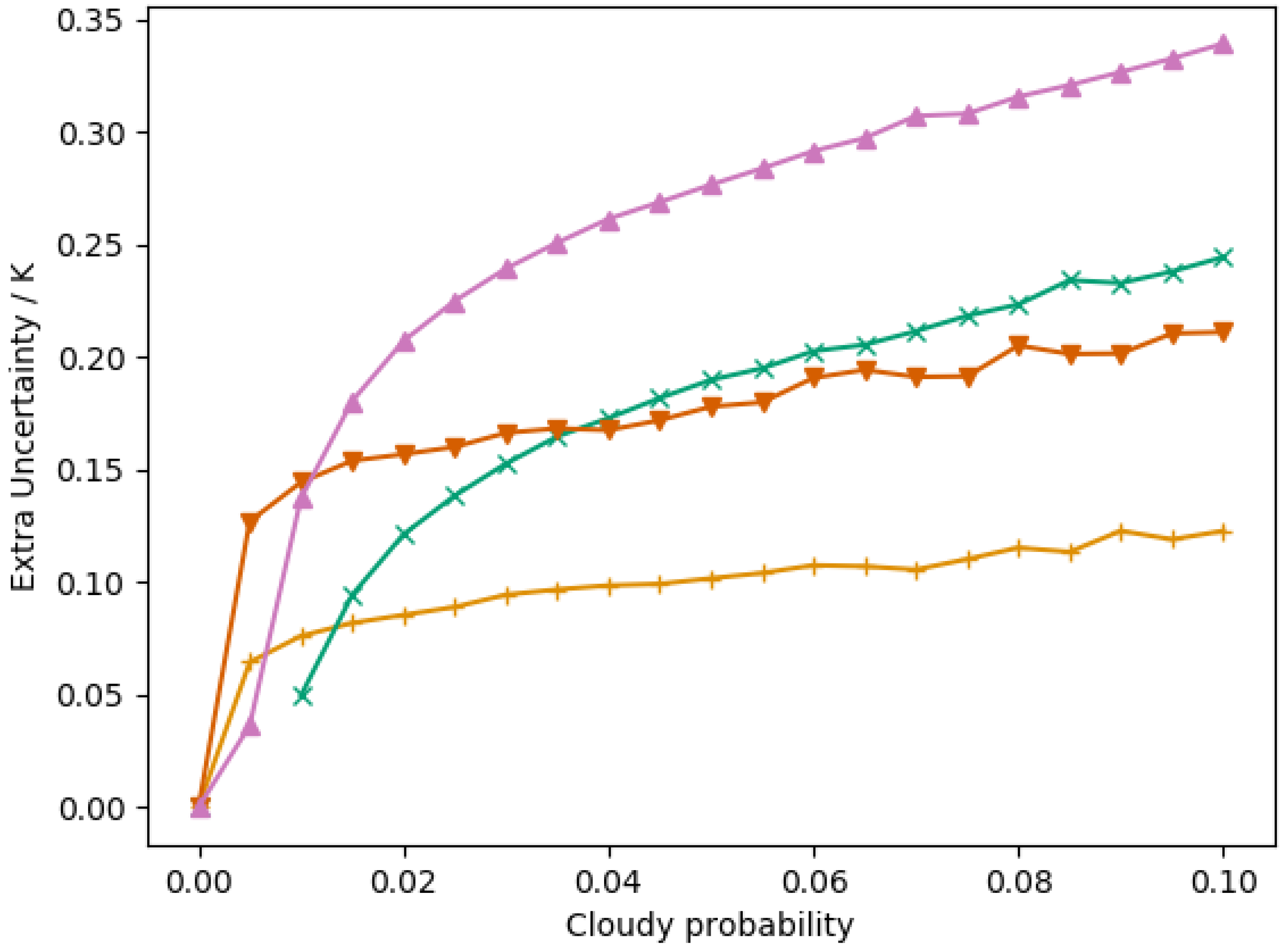Figure 13 shows the standard deviation of the SST differences as a function of cloud probability for the difference retrieval algorithms and shows an increase in standard deviation for a higher likelihood of cloud for quality level 5 pixels. This implies that pixels with a higher cloud probability should have a larger associated uncertainty than a fully clear sky pixel. Again, this is a missing component of uncertainty in the current uncertainty budget. Figure 13 also shows that, in terms of the possible extra component of uncertainty, the D3 (three channel, dual view) retrieval seems to be the most sensitive and the N2 (two channel, nadir view) the least sensitive to the extra source of error related to cloud probability. This also matches with the case looking at the SST difference as a function of cloud probability discussed above, where the D3 algorithm also showed the largest SST differences.

5. Discussion

The S3A/B tandem phase has enabled a detailed analysis of SLSTR radiometric and SST-retrieval performance that would be challenging to reproduce with typical validation techniques, such as using simultaneous nadir overpasses (SNOs) with other satellite sensors for L1 or in-situ measurements for L2 SST. The large tandem dataset covers a comprehensive range of sensor observations; for example, it fully covers the temperature dynamic range, which provides a high-level of fidelity to the comparison. Additionally, common issues encountered in other validation methodologies, such as temporal, spatial or geometric mismatch, are significantly minimised by the tandem configuration. It is also important to note, in the context of the remainder of the S3 mission, that such direct comparison of SLSTR-A and B will not be possible once the instruments are on their nominal orbit, so, in this context, the tandem phase is crucial to ensure interoperability going forward.

The results from this analysis can be split into two different topics: first, those related to the analysis of the measurements themselves, and, second, those related to the provided estimates of uncertainty—these are discussed separately below.

5.1. Measurement Analysis

The comparison of L1 TIR radiometry has shown that at a global level SLSTR-A and B agree well, with mean differences of order 10 $\mathrm{m}$$\mathrm{K}$ observed in the S7, S8 and S9 channels for oblique and nadir views. A particular advantage of the tandem configuration for SLSTR at L1 is that it facilitates a direct comparison of the oblique view in its native geometry, which is not possible when comparing to other nadir-viewing sensors. Additionally, as mentioned, match ups are readily available right across the sensors’ dynamic ranges. The combination of these factors allowed for a detailed analysis of performance as a function of scene temperature in both the nadir and oblique views. In the oblique view, this has confirmed a suspected nonlinearity effect in one or both of SLSTR-A/B that trends across the dynamic range. This apparent stray-light issue, originally observed in the pre-flight data, is at a level that significantly exceeds the estimated measurement uncertainty and so a correction should be applied. This study investigated a potential empirical correction, which was found to perform well for the tandem data, further analysis of which is recommended.

The observed L1 differences were found to be relatively stable in the period following the end of SLSTR-B commissioning activities and the modification of the SLSTR-A detector set-point temperature. This apparent consistency, combined with the low overall biases described above, make the constellation a good candidate for the retrieval of accurate Climate Data Records.

The time series results also highlight the importance of tandem phase planning to its success as a validation exercise. Necessary commissioning phase activities should be scheduled so that they occur prior to a sufficiently long tandem phase. Clear temporal separation of significant events would ease the disentangling of the effects of the S3A and B mission activities. Furthermore, the duration of the tandem phase must ensure that there is a chance for analysis after the instruments have stabilised.

In terms of the SST retrievals, the tandem phase data have shown that using two independent, temporally-coincident observations allows a study of the detail of the retrieval process to a level that would be very difficult using more standard validation techniques. With the tandem data, it is possible to see small biases between the sensors at the hundredth of degree level even for the lower quality level data. This comparison has shown that the use of the SLSTR-A retrieval algorithm on SLSTR-B data (as is currently the case) introduces small but real biases in the highest quality level data. There are two conclusions to be drawn from this. Not only does the tandem phase allow a detailed study of very small differences in the SST retrieval process, but the fact that using the wrong set of retrieval coefficients led to such small differences shows that the two SLSTR instruments are indeed very closely matched (as described in the L1 analysis above) and also means that the Sentinel-3 series will be a good benchmark for climate-related SST studies.

The tandem data have also allowed a detailed study of the SST retrievals as a function of GHRSST quality level. This has shown that work needs to be done to harmonise the different retrieval algorithms (N2, N3, D2, D3) across the different quality levels and has shown that and the N2 retrieval is an outlier. The tandem data are also highlighting questions related to the meaning of the GHRSST quality levels. In particular, the data are showing that in a small but significant number of cases the GHRSST quality level can change between the SLSTR-A and SLSTR-B observation after only a 30 s time gap. This then means that the concept of a GHRSST quality level is not necessarily fixed for a given location but may be more fluid. For example, from the analysis above, it seems that cloud proximity has a role to play in determining the observed quality level giving rise to more variability in assigning a given quality level near cloudy regions. Secondly, there is evidence for variations in quality level directly related to measurement uncertainty which then means that there is a small but real uncertainty in the quality level itself. This is the first time that any sort of analysis on the possible variable nature of the GHRSST quality level has been done and again is only possible with tandem data where two measurements of essentially the same location at close to the same time are taken.

Lastly, the tandem data are providing information of the impact of variable amounts of detected cloud in the SST estimates. In particular, the tandem data are showing evidence of a small amounts of cold bias caused by cloud in the data within the same quality level. Therefore, for the first time, it should be possible to formulate a model of SST bias as a function of the cloud probability once the SLSTR-B SSTs are fully formulated. Again, this sort of work is only really possible using tandem data as the changes seen are related to changes in the local environment (e.g., clouds) rather than in changes in the underlying SST itself and so processes such as cloud contamination can be studied in a way not possible with other techniques.

5.2. Uncertainty Validation

A key objective of this study was to apply metrological principles to the comparison of satellite observations. As previously described, within this context, uncertainty validation provides the key result of the comparison exercise, quantitatively determining if the sensors are meeting their expected performance. Since uncertainty information is available in both the SLSTR L1 and L2 products, such analysis was possible for the radiometric and SST data looked at in this study. The valuable quantitative conclusions that have been drawn on the basis of such uncertainty analysis demonstrates a key utility of the provision uncertainty information in satellite data products.

At L1, it was found that the estimated uncertainties were reasonable for the S8 nadir channel and S7 channel in both views. Aside from the stray light issue previously described for the S8 and S9 oblique channels, the consistent 50 $\mathrm{m}$$\mathrm{K}$ difference for the S9 channel was not explained by the uncertainties. The latter could be due to uncorrected detector temperature sensitivity, which should be further investigated. For the L2 SST data, the analysis was somewhat limited by a large component of covariance between SLSTR-A and B observations, but it has been shown that the theoretical uncertainties as provided likely need updating. At the very least, the N2 and D3 theoretical uncertainties will need updating being seemingly too large and too small, respectively.

Beyond the current uncertainties in the data, the tandem data are also showing that there may be missing components of uncertainty in the SST data. It is clear from the statistics that in moving to a lower quality level there is an increase in the standard deviation that an extra component of uncertainty should be associated with a lower quality level. While this may seem obvious, with the tandem data, we can begin to provide an estimate of how large such a component should be and therefore we have the possibility of adding a quality-level-related uncertainty estimate. In addition, on top of this, the tandem data are also showing evidence of the extra uncertainty associated with the cloud probability, which is again a currently missing component of uncertainty. While the data used is not sufficient to pin this down fully because the SLSTR-B SST is not derived using the correct retrieval coefficients, the use of tandem data will clearly have a role in estimating a more complete SST theoretical uncertainty in the future.

6. Conclusions

In conclusion, the tandem phase has proved to be a valuable addition to the understanding of the SLSTR L1 and L2 SST data. Looking at the same location twice in a very short period of time with essentially the same viewing geometry allows for a comparison with a level of detail challenging to achieve with other common validation methodologies. Additionally, applying metrological principles to the comparison, facilitated by the availability of the uncertainties in the L1 and L2 SST products, has enabled a more quantified analysis of the derived results.

For the L1 radiometric comparison, good performance was found in nadir view TIR channels S7, S8 and S9, and the oblique view S7. However, in the S8 and S9 channels, in the oblique view, a strong nonlinearity effect was found, as previously observed in the pre-flight analysis. A correction was proposed for this effect, which is recommended for further investigation.

The tandem data have also been useful in finding small differences in SST, and by looking at them as a function of difference aspects of the SST retrieval process (e.g., retrieval algorithm, quality level, cloud probability), some new processes related to SST bias and uncertainty have been identified. These include the nature of the SST retrieval as a function of quality level as well of as a function of cloudy probability, both of which have not been studied at this level of detail before. The Tandem data have also proven to be useful in finding problems with the operational retrievals related to the current set of coefficients and should be included in subsequent updates to the SST retrieval algorithms.

References

- Donlon, C.; Berruti, B.; Buongiorno, A.; Ferreira, M.H.; Féménias, P.; Frerick, J.; Goryl, P.; Klein, U.; Laur, H.; Mavrocordatos, C.; et al. The Global Monitoring for Environment and Security (GMES) Sentinel-3 mission. Remote Sens. Environ. 2012, 120, 37–57. [Google Scholar] [CrossRef]
- Coppo, P.; Ricciarelli, B.; Brandani, F.; Delderfield, J.; Ferlet, M.; Mutlow, C.; Munro, G.; Nightingale, T.; Smith, D.; Bianchi, S.; et al. SLSTR: A high accuracy dual scan temperature radiometer for sea and land surface monitoring from space. J. Mod. Opt. 2010, 57, 1815–1830. [Google Scholar] [CrossRef]
- Merchant, C. Sea Surface Temperature (SLSTR) Algorithm Theoretical Basis Document; Report; ESA: Paris, France, 2012. [Google Scholar]
- Lamquin, N.; Woolliams, E.; Bruniquel, V.; Gascon, F.; Gorroño, J.; Govaerts, Y.; Leroy, V.; Lonjou, V.; Alhammoud, B.; Barsi, J.A.; et al. An inter-comparison exercise of Sentinel-2 radiometric validations assessed by independent expert groups. Remote Sens. Environ. 2019, 233, 111369. [Google Scholar] [CrossRef]
- Mittaz, J.; Merchant, C.J.; Woolliams, E.R. Applying principles of metrology to historical Earth observations from satellites. Metrologia 2019, 56, 032002. [Google Scholar] [CrossRef]
- Gorroño, J.; Fomferra, N.; Peters, M.; Gascon, F.; Underwood, C.I.; Fox, N.P.; Kirches, G.; Brockmann, C. A radiometric uncertainty tool for the Sentinel-2 mission. Remote Sens. 2017, 9, 178. [Google Scholar] [CrossRef]
- Gorroño, J.; Hunt, S.E.; Scanlon, T.; Banks, A.; Fox, N.; Woolliams, E.; Underwood, C.; Gascon, F.; Peters, M.; Fomferra, N.; et al. Providing uncertainty estimates of the Sentinel-2 top-of-atmosphere measurements for radiometric validation activities. Eur. J. Remote Sens. 2018, 51, 650–666. [Google Scholar] [CrossRef]
- Smith, D.; Hunt, S.E.; Woolliams, E.; Etxaluze, M.; Peters, D.; Nightingale, T.; Mittaz, J. Traceability of the Sentinel-3 SLSTR Level-1 Infrared Radiometric Processing. In Preparation.
- Casey, K.; Donlan, C. The Recommended GHRSST Data Specification v2.0; Report; Group for High Resolution Sea Surface Temperature: Leicester, UK, 2016. [Google Scholar]
- Smith, D.; Barillot, M.; Bianchi, S.; Brandani, F.; Coppo, P.; Etxaluze, M.; Frerick, J.; Kirschstein, S.; Lee, A.; Maddison, B.; et al. Sentinel-3A/B SLSTR Pre-Launch Calibration of the Thermal InfraRed Channels. Remote Sens. 2020, 12, 2510. [Google Scholar] [CrossRef]
- JCGM. Evaluation of Measurement Data—Guide to the Expression of Uncertainty in Measurement; JCGM: Paris, France, 2008; Volume 100. [Google Scholar]
- Tomazic, I.; O’Carroll, A.; Hewison, T.; Ackerman, J.; Donlon, C.; Nieke, J.; Andela, B.; Coppens, D.; Smith, D. Initial comparison between Sentinel- 3A SLSTR and IASI aboard MetOp-A and MetOp-B. GSICS Q. 2016, 10, 1–3. [Google Scholar] [CrossRef]
- Bulgin, C.; Embury, O.; Merchant, C. Sampling uncertainty in gridded sea surface temperature products and Advanced Very High Resolution Radiometer (AVHRR) Global Area Coverage (GAC) data. Remote Sens. Environ. 2016, 177, 287–294. [Google Scholar] [CrossRef]
Figure 1.
Example of a SLSTR-A scene from the tandem phase in the nadir view, S8 channel (left), and the difference between this scene and the corresponding SLSTR-B scene (right) separated in time by 30 (data: 13 August 2018).
Figure 2.
Density of differences between SLSTR-A and B gridded data in the S8 channel, nadir view as a function of the standard deviation of SLSTR-A grid cell pixel values, (data: 3 September 2018). The solid black line shows the filtering threshold of 2 , which is used to select for homogeneous grid cells.
Figure 3.
Distribution of uncertainty-normalised differences between SLSTR-A and B gridded data in the linear detector region (data: 3 September 2018). The solid line vertical line indicates the distribution mean, the dashed vertical lines indicate the distribution standard deviation. The black curve indicates a normal distribution with a standard deviation of 1, centred on the mean of the difference distribution.
Figure 4.
Differences between SLSTR-A and SLSTR-B for thermal infrared channels in the oblique and nadir views plotted as functions of binned scene radiance, error bars indicate propagated instrument calibration uncertainties at , the two dashed vertical lines indicate the temperatures of SLSTR’s blackbody calibration targets (data: 3 September 2018).
Figure 5.
Differences between SLSTR-A and SLSTR-B for channels S8 and S9 in the oblique view plotted as functions of binned scene radiance, as in
Figure 4, with the proposed stray light correction applied. Error bars indicate propagated instrument calibration uncertainties at
, with no additional uncertainty corresponding to the straylight correction applied. The two dashed vertical lines indicate the temperatures of SLSTR’s blackbody calibration targets (data: 3 September 2018).
Figure 6.
Time series of differences between SLSTR-A and SLSTR-B TIR channels during S3A/B tandem phase. Data points represent radiometric differences observed for days of night-time gridded data at 280 K. The solid lines provide the temperature of SLSTR-A and B during this period.
Figure 7.
SST differences for different retrieval algorithms (N2—Orange, N3—Green, D2—Brown, D3—Purple) for excellent (QL5) cases and a 30 s time difference.
Figure 8.
Distributions of the distance in pixels of the nearest SLSTR-A quality level 3 pixel from a quality level 5 pixel for locations where (left-hand side) the quality level doesn’t change between SLSTR-A and SLSTR-B and (right-hand side) for when the quality level changes from a 5 to a 3 in SLSTR-B.
Figure 9.
SST difference histograms for pixels with an SLSTR-A quality level of 5 and an SLSTR-B quality level of 3.
Figure 10.
Left-hand plot shows the mean SST difference between SLSTR-A and SLSTR-B as a function of cloud probability for quality level 5 data together with the standard error on the mean where the data has been normalised to the zero cloud probability case. Different colours show different retrieval algorithms (N2—Orange (+), N3—Green (×), D2—Brown (▽), D3—Purple (△)). Right-hand plot shows the same normalised data plotted as a function of the cloud probability difference.
Figure 11.
Theoretical uncertainty (Blue) and associated SSES standard deviation (Orange) for the quality level 5 data for the different retrieval algorithms.
Figure 12.
Theoretical uncertainty-normalised distributions for quality level 5 pixels for the different retrieval algorithms.
Figure 13.
Standard deviation of SST differences for quality level 5 data as a function of cloud probability for N2, N3, D2 and D3 algorithms (see
Figure 10 for key). The plot has normalised the curves to zero cloud probability.