Article

Tree Line Identification and Dynamics under Climate Change in Wuyishan National Park Based on Landsat Images

1
Department of Ecology, College of Biology and the Environment, Nanjing Forestry University, Nanjing 210037, China
2
Co-Innovation Center for Sustainable Forestry in Southern China, Nanjing Forestry University, Nanjing 210037, China
3
Wuyishan National Park, Wuyishan 354300, China
*
Author to whom correspondence should be addressed.
Remote Sens. 2020, 12(18), 2890; https://doi.org/10.3390/rs12182890
Submission received: 4 August 2020 / Revised: 3 September 2020 / Accepted: 4 September 2020 / Published: 6 September 2020

Abstract

:
The alpine tree line ecotone, reflecting interactions between climate and ecology, is very sensitive to climate change. To identify tree line responses to climate change, including intensity and local variations in tree line advancement, the use of Landsat images with long-term data series and fine spatial resolution is an option. However, it is a challenge to extract tree line data from Landsat images due to classification issues with outliers and temporal inconsistency. More importantly, direct classification results in sharp boundaries between forest and non-forest pixels/segments instead of representing the tree line ecotone (three ecological regions—tree species line, tree line, and timber line—are closely related to the tree line ecotone and are all significant for ecological processes). Therefore, it is important to develop a method that is able to accurately extract the tree line from Landsat images with a high temporal consistency and to identify the appropriate ecological boundary. In this study, a new methodology was developed based on the concept of a local indicator of spatial autocorrelation (LISA) to extract the tree line automatically from Landsat images. Tree line responses to climate change from 1987 to 2018 in Wuyishan National Park, China, were evaluated, and topographic effects on local variations in tree line advancement were explored. The findings supported the methodology based on the LISA concept as a valuable classifier for assessing the local spatial clusters of alpine meadows from images acquired in nongrowing seasons. The results showed that the automatically extracted line from Landsat images was the timber line due to the restriction in spatial autocorrelation. The results also indicate that parts of the tree line in the study area shifted upward vertically by 50 m under a 1 °C temperature increase during the period from 1987 to 2018, with local variations influenced by slope, elevation, and interactions with aspect. Our study contributes a novel result regarding the response of the alpine tree line to global warming in a subtropical region. Our method for automatic tree line extraction can provide fundamental information for ecosystem managers.

Graphical Abstract

1. Introduction

The alpine tree line ecotone provides important ecosystem services (hotspots of biodiversity [1], slope stability, high-quality water for downstream areas [2], nutrient input, and carbon sequestration for lower-elevation ecosystems [3]) and reflects interactions among climate, species ecology, physiography, and physiology [4,5]. It is also very sensitive to climate change [6,7,8] and is one of the most sensitive bio-indicators of past climate fluctuations [9]. Thus, the dynamics of tree line ecotones are useful indicators of vegetation response to climate change [10,11].

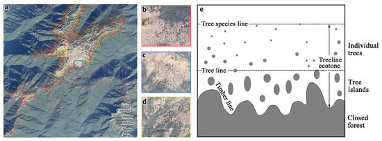
1.1. Alpine Tree Line Ecotone

The alpine tree line ecotone is defined as a forest–grassland or forest–tundra transition boundary between a subalpine forest and a treeless grassland or between a subalpine forest and a treeless tundra [12,13]. The upper boundary of the alpine tree line (tree species line; Figure 1) is the higher elevational limit of individual tree establishment and growth (Figure 1). This limit is generally set by the minimum temperature for tree growth at high altitudes [14]. While the lower boundary of the alpine tree line is often referred to as the timber line, the upper boundary of the closed subalpine forest is also called the timber line (Figure 1) [2]. The alpine tree line ecotone is the belt region between the tree species line and the timber line of a closed forest; the tree line often refers to the transition line between tree islands and isolated individual trees (Figure 1) [2].
Among studies that have focused on the movement of tree lines in the past century, several have observed that tree lines move upward in mountainous regions [10,12,16,17,18,19,20,21,22,23,24], while others have not observed any clear upward [25,26,27] or downward [2,28,29] movement of tree lines. Four reasons have been cited to explain these inconsistent research findings. First, the research time period is typically short. Time scale (short period, median period, and long-term) is very important for tree line advancement research [30]. As Lloyd [31] indicated, the mean time lag between initial tree recruitment and forest development is 200 years, but study duration have comprised a fraction of this. Second, the intensity of upward tree line shift varies between climate zones, largely due to the uneven global climate change effects [32], as well as significantly different dominant vegetation species and communities correlated with climate zones [33]. Third, historical anthropogenic disturbances (e.g., deforestation) have caused upward tree line shifts [16,24], where they may be carried out due to climate conditions [17]. This creates an enormous challenge in studying tree line upslope advance responses to climate change [2]. Finally, temperature has not been a primary factor dominating tree line upward advancement under long-term global warming until now [28]. Even within a single area, strong local variations in tree line shifts have been observed in many studies [10,12,20,34,35]. Therefore, it is important to improve our understanding of tree line shifts with climate change and to explore other environmental factors that can cause local variation in tree line advancement. The long-term historical mapping of tree lines with detailed local spatial information, as opposed to studies in several elevational transitions [12,23,36,37], is fundamental for modern studies of tree line shifting.

1.2. Remote Sensing Applications for Tree Line Dynamics
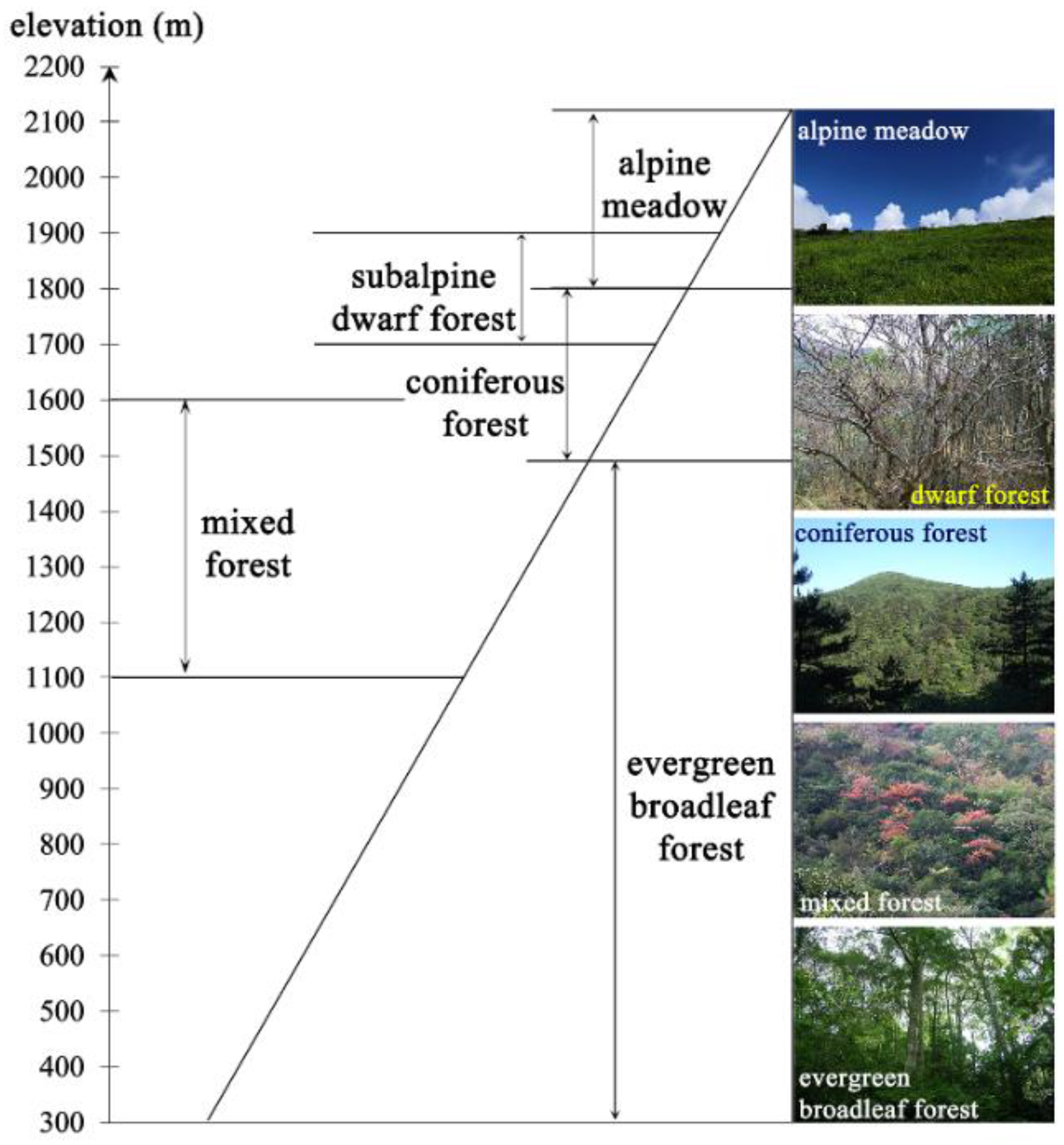
Traditional research methods for monitoring tree line ecotone dynamics use either tree-seedling demographics [38], natality and mortality [20,37,39,40], recruitment [41,42], establishment [9,10], radial growth [29,43,44,45,46,47], age structure [8,12,41,48,49], population density [48,50,51], or tree islands [52] as indicators. Alternatively, these methods compare current field observations and historical documents to measure tree line advancements [23,53], or they even compare pollen and vegetation remnant analyses to reconstruct past tree line patterns [54,55,56,57,58]. However, it is difficult to evaluate temporal changes in tree line positions while incorporating local variations using these traditional research methods.
Remote-sensing approaches have the potential to capture spatial variations in tree line positions and enable long-term analyses of upward tree line advancement. Previous studies applying remote-sensing methods to tree line ecotones have followed one of three directions: evaluating biophysical parameters in tree line ecotones, measuring topographic factors that impact tree line dynamics, or measuring tree line position and shifting. Biophysical parameter research has used temporal canopy cover information [13,21,59], tree density [60], species abundance [61,62,63], fraction of absorbed photosynthetically active radiation (FAPAR), and vegetation water content [64] measured from remote-sensing data (or directly from temporal changes of vegetation indices [65,66]) as indicators for tree line dynamics. Second, digital elevation models (DEMs) have been applied to extract parameters to analyze topographic effects on tree line position and tree density along the tree line [13,67]. Finally, the classification of forest and non-forest areas from moderate-resolution imagery [13,16,17,24,68] and the detection of individual trees and tree islands from high-resolution imagery [21,69,70,71,72], aerial photos, or Lidar data [73,74] have been reported in the literature with regard to measuring the spatial variation of tree line position and the temporal change of tree line advancement. Nevertheless, few studies have attempted to use a searching window to find the highest-elevation forest pixels in order to identify potential tree line locations, as determined by climate factors instead of anthropogenic disturbance [17].
However, it remains a challenge to extract temporal changes in tree line position using remotely sensed images due to mismatches between ecological conditions and remote-sensing outputs. One issue comes from spatial resolution and the length of time over which tree line dynamics are studied. Long-term remote-sensing imagery (e.g., Landsat with a 30 m spatial resolution) has a limited ability to analyze the upward advancement of a tree line due to climate change if the shift is less than a single pixel’s breadth (e.g., the tree line of the Khibiny Mountains in Russia advanced about 27 m vertically over 55 years [21]). However, when the slope is less than 45°, the horizontal distance is larger than vertical distance, which gives Landsat imagery the potential to monitor tree line advancement within its 30 m spatial resolution.
Another mismatch is that the direct output of remote-sensing classification from forest and non-forest pixels/segments is usually sharp boundaries between alpine meadows and forests instead of the location of a tree line ecotone, even when the spatial resolution of the image is high enough to detect tree islands. Therefore, it is unclear which ecotone type (i.e., tree species line, tree line, or timber line; Figure 1) is extracted from remote-sensing images. Moreover, results from conventional pixel-based classification approaches (e.g., supervised or decision-tree classification) normally include erroneous land cover, which is a challenge for long-term temporal change analysis [75]. Maintaining a consistent remote-sensing dataset of spectral reflectance is a further challenge that must be overcome to ensure long-term the consistency of remote-sensing applications in ecosystems, especially with a background of rapid global change [76]. Thus, remote sensing has its own particular challenges in measuring tree line advancement with climate change due to the heterogeneity of ecotones caused by individual trees and tree islands (Figure 1). Therefore, it often requires expert knowledge to conduct post-classification analysis and change detection to identify land-cover errors in order to properly attribute land-cover change [75].
There is also inconsistency in detecting temporal change from remote-sensing images. Studies have used pixel clustering on homogeneous segments with thresholding algorithms prior to classification to reduce erroneous results [77]. Local indicator of spatial association (LISA), another method that captures spatial clusters, performs well as a classifier for ecological research (e.g., burn severity [78] and vegetation fragmentation in urban areas [79]). However, LISA, as a geostatistical technique, is still rarely used as a classifier of remotely-sensed images even though it has been shown to be more accurate than conventional classification approaches [77]. These studies have also shown that introducing spatial weights (a major parameter of LISA) would improve the temporal consistency of land-cover classification from remote-sensing images [80]. For tree line mapping, LISA may have great potential to distinguish alpine meadows from closed forests and tree line ecotones because high spatial autocorrelation is common within alpine meadows, in contrast to heterogeneous tree line ecotones and closed forests.
This study aimed to develop a new detection method based on the LISA concept in order to detect tree line position and dynamics from Landsat imagery. The specific objectives were (1) to use LISA to develop a new method of automatically identifying tree line location from Landsat imagery and explaining detected ecotone types, (2) to evaluate the dynamics of tree line positioning over 30 years, (3) to analyze the response of upward tree line shifts to climate change, and (4) to explore topographic effects on local variations of tree line advancement.

2. Study Area

The study area was in the boundary of Wuyishan National Park in the northern Fujian and Jiangxi Provinces, China (27°49′–27°53′N, 117°45′–117°49′E; Figure 2). This area, characterized as a subtropical evergreen broad-leaf forest, has been identified as important for its contribution to world biodiversity [81]. Wuyi Mountain (Wuyishan) is included in the World Natural and Cultural Heritage list (23rd Session of the World Heritage Committee; December 1999) [82]. Wuyishan was first declared a national park in 2017, and its area includes Wuyishan National Nature Reserve (NNR; 565.27 km2), the Nine-Bend Stream Ecological Protection Area (NEPA; 353.32 km2), and the Wuyishan National Scenic Area (NSA; 64 km2) [83].
The region has a typical humid subtropical monsoon climate that is characterized by warm summer temperatures, cool winter temperatures, and abundant annual precipitation [84]. Across the elevation gradient in the study area, the mean annual rainfall is approximately 2050, 2530, and 2820 mm at 1200, 1600, and 2000 m a.s.l., respectively, with approximately 70% of the precipitation falling during the growing season (from March to August) [85]. Nearly all the precipitation is rainfall instead of snowfall, however, extreme weather events (e.g., El Nino effects) can cause snowfall in winter time (e.g., strong snowfall in 2008). The annual mean temperature is 13, 11, and 9 °C at 1200, 1600, and 2000 m a.s.l., respectively [86]. The month with the lowest temperature is January or February, and the average temperature of the coldest month is 7.6 °C. There is no prevailing wind direction at the top of the mountain due to valley wind from different directions, but westerly and northwesterly winds are more frequent in the winter. The soil type is classified as yellow-red soil based on the Chinese soil classification system, which is equivalent to Ultisol in the US Department of Agriculture (USDA) soil taxonomy [87]. Along the altitude gradient from high to low, there are five distinct vegetation communities (Figure 3): the alpine meadow (AM; Figure 2b), the subalpine dwarf forest (DF; Figure 2b), the subalpine coniferous forest (CF; Figure 2b), the mixed forest, and the evergreen broad-leaf forest [88,89]. Along the tree line, the alpine meadow is dominated by Miscanthus sinensis, Deyeuxia arundinacea, and Molinia japonica; the subalpine dwarf forest is dominated by Buxus sinica (Rehd. et Wils.) and Cheng ex M. Cheng subsp. sinica var. parvifolia M. Cheng, and the coniferous forest is dominated by Pinus taiwanensis Hayata, Tsuga chinensis (Franch.), Pritz. var. tchekiangensis (Flous) Cheng et L.K. Fu, and Pinus massoniana Lamb. Overall, the climate conditions characterized by low temperature, low pressure, and strong wind formed the alpine meadow in the study area. In some areas, the tree line is dominated by a transactional ecotone between the dwarf forest and the alpine meadow, while in other areas, the tree line is dominated by a transactional ecotone between the coniferous forest and the alpine meadow (Figure 2b and Figure 3).

3. Materials and Methods

3.1. Datasets

3.1.1. Remotely Sensed Imagery

A total of 54 Landsat Thematic Mapper (TM) images taken from 1987 to 2011, 33 Enhanced Thematic Mapper Plus (ETM+) images taken from 2000 to 2012, and 14 Operational Land Imager (OLI) images taken from 2013 to 2018 were used in this study to extract the tree line in Wuyishan National Park (Table 1). All images had been previously geometrically and atmospherically corrected (Landsat Level-2 from Landsat Collection 1: surface reflectance data, https://www.usgs.gov/land-resources/nli/landsat/landsat-collection-1) when downloaded from the United States Geological Survey (USGS) website (https://earthexplorer.usgs.gov/). Based on the Landsat Collection 1 information, the algorithm used for generating surface-reflectance data of Landsat TM and ETM+ was the Landsat Ecosystem Distribution Adaptive Processing System (LEDAPS), and that of Landsat OLI was the Land Surface Reflectance Code (LaSRC). The spatial resolution of all images was 30 × 30 m, and the projection was UTM (Universal Transverse Mercator) Zone 50N, WGS1984 (World Geodetic System 1984). The digital numbers of the Landsat Level 2 imagery were the reflectance values, with a scale factor of 10,000 (e.g., if the digital number is 4230, the reflectance is 0.423).
In total, 31 historical RGB (Red, Green and Blue: true color composition) images were downloaded from Google Earth (the software used for downloading was BIGEMAP, Chengdu, China). Among these, 26 images with a 16.9 × 16.9 m spatial resolution were acquired from 1987–2016, within which the images from 1991, 1994, 1997, and 2013 were left out due to poor quality. All images were acquired for the same date (31 December) in each year. Another five RGB images were acquired for 23 December 2014 with spatial resolutions of 0.53 × 0.53, 1.06 × 1.06, 2.11 × 2.11, 4.22 × 4.22, and 8.42 × 8.42 m for tree line extraction.
DEM data were from the ASTER (Advanced Spaceborne Thermal Emission and Reflection Radiometer) Global Digital Elevation Model V002 (GDEM2). One DEM image of the study area was downloaded from the NASA website (https://reverb.echo.nasa.gov/reverb/). The spatial resolution for the DEM image was 30 × 30 m, and it was projected as UTM Zone 50N, WGS1984. The horizontal errors for GDEM2 data were −0.13 arc-seconds (east/west shift) and −0.19 arc-seconds (north/south shift). The vertical error was −0.74 m on average, based on Japanese studies, ranging from −5.58 to +15.45 m—with 8.68 m over forest regions and −1.09 m over farmland. The horizontal and vertical accuracy were drawn from an ASTER GDEM2 validation report (https://ssl.jspacesystems.or.jp/ersdac/GDEM/ver2Validation/Summary_GDEM2_validation_report_final.pdf).

3.1.2. Climate Data

Climate data from 1984 to 2017, including monthly accumulated precipitation and mean temperature, were acquired from meteorological station no. 58730 (27°27′36″N, 118°1′12″E).

3.2. Methods

To develop a new method for extracting tree lines and identifying the type of extracted lines (i.e., tree line, timber line, or tree species line), potential available bands for ecotone detection were tested for automatic tree line identification from Landsat series images (Figure 4). The optimal season for tree line extraction (i.e., acquisition time for Landsat images) was also evaluated. To achieve our objectives, climate impacts on upward tree line shifts, as well as local variations in the intensity of upward tree line movement, were measured. This research also explored the topographic effects on local variations in the intensity of upward tree line shifts.

3.2.1. Automatic Tree Line Extraction from Remote-Sensing Imagery

Preprocessing for all Landsat images, including TM, ETM+, and OLI images, involved clipping to the specific study area and conversion to point format from rasters. LISA (in this study, Anselin Local Moran’s I in the ArcGIS Spatial Statistics toolbox was used as the LISA tool) was then applied to the point data for each Landsat image. LISA was used to capture hot spots (i.e., spatial clusters with high values clustering together) and cold spots (i.e., spatial clusters with low values clustering together) in images based on the concept of spatial autocorrelation between pixels and their surrounding pixels. Taking the normalized difference vegetation index (NDVI) as an example, the alpine meadow had lower NDVI values than other vegetation communities (coniferous and dwarf forests). Therefore, the spatial arrangement for the alpine meadow in images was spatial clusters with low NDVI values clustered together, especially in the grass senescence season when the subalpine forest was evergreen. Thus, low–low clusters (spatial clusters with low values) were selected for the NDVI and near-infrared band (NIR) (the reflectance of NIR was lower for the alpine meadow than for the subalpine forest) of point data with a p-value equal to 0.002 (statistically significant). High–high clusters (spatial clusters with high values) were selected for the blue band (B), green band (G), red band (R), first shortwave infrared band (SWIR1), and second shortwave infrared band (SWIR2) of point data (p-value = 0.002) because the alpine meadow had a higher reflectance in those bands than the subalpine forest (coniferous and dwarf forests in the study area). Statistically, a p-value < 0.05 indicated significance for low–low or high–high clusters. We selected the lowest p-value (0.002 was the lowest p-value result from Anselin Local Moran’s I) to capture the smoother alpine meadow in order to decrease the heterogeneity effects of isolated tree island regions in the tree line ecotone. Postprocessing steps included analyzing the point density (30 × 30 m spatial resolution, consistent with Landsat images) and selecting point densities larger than 0.0005. This processing step converted the selected spatial cluster points (low–low or high–high clusters) into the raster format. The 0.0005 threshold was set to eliminate some small patches of the alpine meadow in the study area; however, it could be adjusted. If it was set lower, more small patches of the alpine meadow would be extracted. Steps also included converting rasters to polygons, eliminating small polygons (area < 2000 m2; this threshold setting, about the area of two pixels, was used to reduce the “salt-and-pepper” effect in images), smoothing polygons, and converting polygons to the tree line (line feature). The shadow effect was an issue when extracting tree lines from NDVI images, so NIR reflectance was used to control it (controlling NIR reflectance values higher than 0.035 to eliminate shadow effects; after exploring the spectral characteristics between mountain shadows and the alpine meadow in the study area, this threshold sufficiently reduced the noise effect of shadows). All steps for extracting the tree line from bands were coded as a Python script, which is available for download (see Supplementary Materials).
To test the impact of the spatial resolution of imagery on tree line extraction, RGB images acquired on 23 December 2014 with spatial resolutions of 1.06 × 1.06, 2.11 × 2.11, 4.22 × 4.22, and 8.42 × 8.42 m were tested and compared.

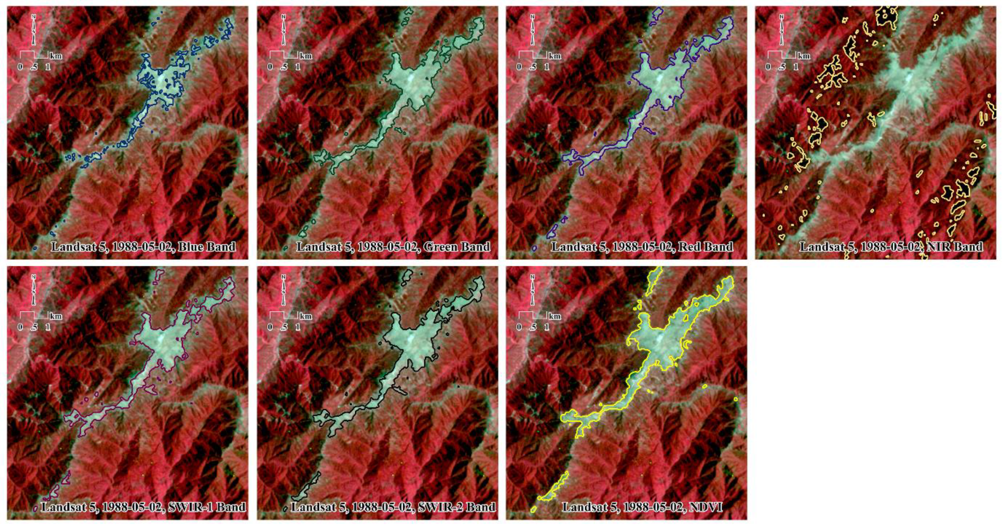
3.2.2. Selecting Optimum Band and Season for Tree Line Extraction

The strategy for selecting the optimum band and season for tree line extraction was to compare all extraction results with the reference RGB image acquired in the same year. The boundaries between different vegetation communities do not change much within a year, so the variations of tree line extraction from different bands acquired for the same year were caused by extraction accuracy. It is necessary to choose the optimum extraction band and season for consistent temporal analysis. Vegetation phenology causes a high variation of spectral signals for the same vegetation type (e.g., this was noteworthy for the alpine meadow—the spectral signals of evergreen vegetation communities do not change much within a year), which may result in different extraction results even with images acquired in the same year. In addition, an accuracy assessment with the reference RGB image (spatial resolution of 0.53 × 0.53 m, with individual trees visible) acquired on 23 December 2014 was conducted for tree line extraction from the Landsat OLI images acquired on 2 January, 17 October, and 20 December 2014 to select the optimum extraction season.

3.2.3. Identification of Type of Extracted Tree Line

The tree line ecotone in the study area is transitional (the mosaic region of the alpine meadow and tree islands or individual trees; see Figure 1) between the coniferous forest and the alpine meadow or between the dwarf forest and the alpine meadow. In other words, the tree line ecotone potentially has an upper boundary (tree species line; Figure 1), lower boundary (timber line; Figure 1), and tree line (boundary between tree islands and individual trees; Figure 1). However, it is interpreted as a boundary line between the alpine meadow and forest when using remote-sensing imagery. Therefore, it is important to identify which line (timber line, tree line, or tree species line) is being extracted based on the LISA concept used in this study. The extracted line was identified visually by comparison to RGB images in which individual trees and tree islands were clearly visible at a high spatial resolution (0.53 × 0.53 m).

3.2.4. Time-Series Analysis and Segmented Linear Regression for Climate Data

To accurately capture the annual trend of temperature change, the seasonal effects of monthly mean temperature were reduced by a time-series analysis (TSA) using the Extensible Time Series (xts) package in the R software (https://www.r-project.org/). From this, the annual temperature trend data were analyzed using the segmented linear relationship with the Segmented package in the R software. The segmented linear relationship, which is also called the broken-line relationship, is widely used in ecological research [90]. In this study, the segmented linear relationship was used to analyze thresholds in temperature change trends and to evaluate the alpine meadow area trend.

3.2.5. Topographic Effects on Local Variations of Upward Tree Line Shift

The topographic factors of aspect, slope, and contour were estimated from DEM data using surface analysis in the ArcGIS software. To analyze the topographic effects on local variations of tree line advancement along an altitudinal gradient with climate change, a t-test was used to compare whether there was a significant difference of slope and elevation between stable and rapidly upward shifting tree lines. A two-way ANOVA was conducted to determine whether there were significant differences of slope and elevation between different tree line types (stable and advanced tree line) and aspects (flat, north, northeast, east, southeast, south, southwest, west, and northwest). The samples used for testing topographic effects were from the pixel values (slope, elevation, or aspect) where the tree line was located for the stable tree line, as well as from all pixels in the location between the current advanced tree line and previous tree lines during the study period.

4. Results

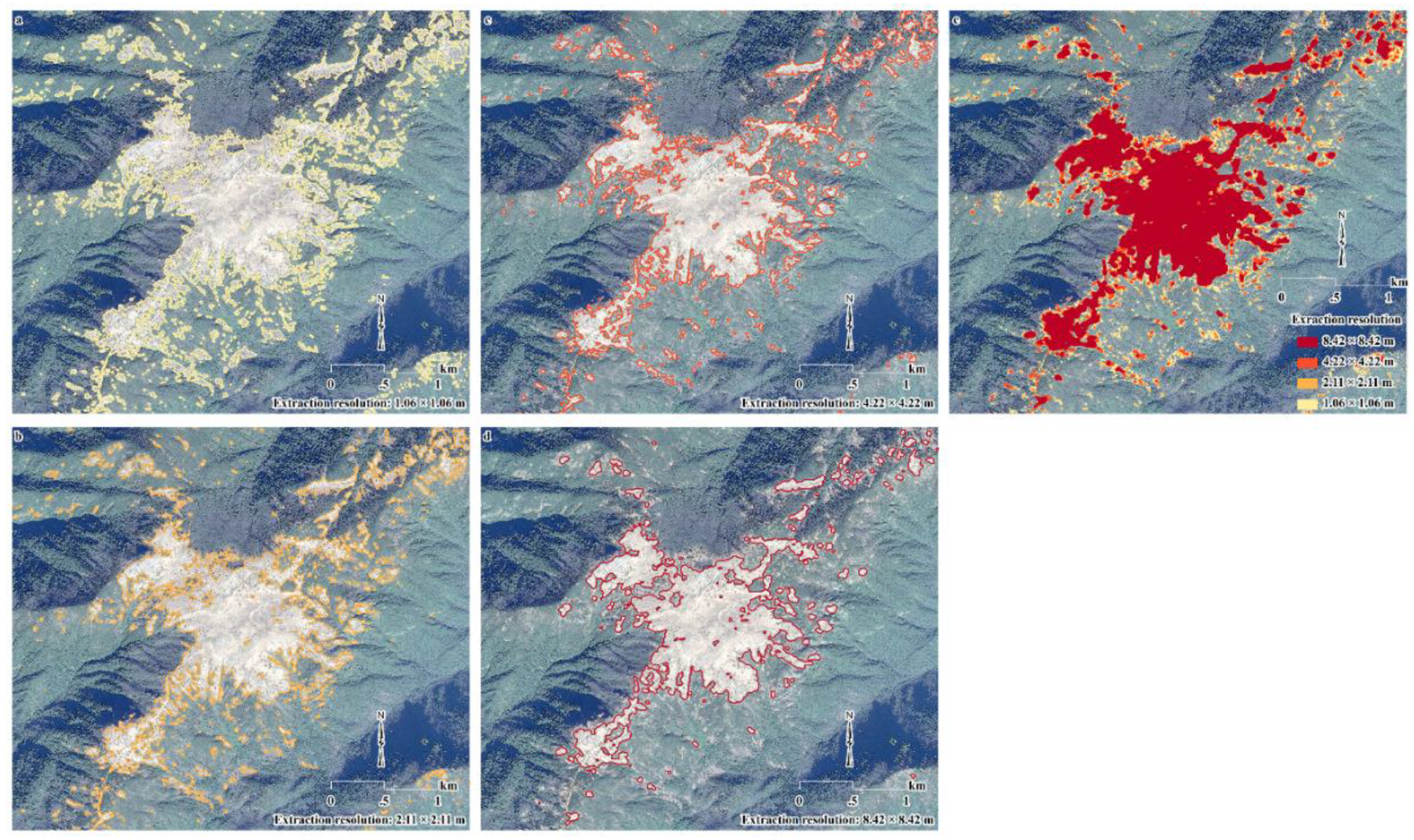
4.1. Automatic Extraction of Tree Line from Landsat Imagery

With our methodology for automatic tree line extraction, the NDVI performed best of all bands based on the visual comparison with the RGB reference images (16.9 × 16.9 m spatial resolution) for each year (Figure 5). According to the spectral signatures of different vegetation communities around the tree line ecotone (alpine meadow, subalpine coniferous forest, and subalpine dwarf forest in the study area), the use of the NIR band to detect the alpine meadow was the least accurate. Therefore, significant low–low clusters (low values significantly clustered) from spatial autocorrelation analysis were selected for the alpine meadows. However, the results from the NIR bands were greatly influenced by mountain shadows (Figure 5) because they had even lower reflectance in the NIR bands than the alpine meadow. Based on these constraints, the reflectance values of B, G, R, SWIR1, and SWIR2 in the alpine meadow were higher than those of other vegetation communities because dead materials cause higher reflectance in the B, G, and R bands than green vegetation and they hold less water content, resulting in higher reflectance values in the SWIR1 and SWIR2 bands. Compared to tree line extraction from the NDVI, extraction results from B, G, R, SWIR1, and SWIR2 showed patchiness, especially the B band, due to strong atmospheric effects. Regardless, the NDVI performed optimally in extracting the tree line and was only slightly affected by mountain shadows. Therefore, the shadow effects of extraction from the NDVI band were controlled by reflectance from the NIR band because its reflectance of shadow was much lower than in alpine meadows. Reflectance values larger than 0.035 (the default value set in Python script) in the NIR band were selected to reduce the shadow effects as an additional postprocessing step.
According to tree line extraction results from available cloud-free Landsat images, the optimal extraction time was from late October to early May (Figure 6; see tree line extraction from the NDVI of all images from Landsat series in Supplementary Material A). From the images acquired during June to September, only the disturbed region (the area surrounding the tourist trail to the mountain top) was extracted (Figure 6). This optimal extraction season is consistent with the senescent phenology period of the alpine meadow. The alpine meadow in the study area starts to green up in early May and senesce in late September. Therefore, the extracted meadow area from 13 May was significantly smaller than that from 3 May (Figure 6), and it gradually increased from 25 September to 21 October (Figure 6). Based on the accuracy assessment results with the reference RGB image acquired on 23 December 2014 (0.53 × 0.53 m spatial resolution), the tree line extracted from the Landsat OLI images acquired on 2 January 2014 (overall accuracy = 98%; kappa coefficient = 95.77%) and 20 December 2014 (overall accuracy = 98%; kappa coefficient = 95.80%) was better than that acquired on 17 October 2014 (overall accuracy = 88.67%; kappa coefficient = 75.30%—see distribution of points and error matrix for accuracy assessment in Supplementary Material B). Therefore, images acquired in the completely senescent season of the alpine meadow were the best choice for tree line extraction for each year. Based on this criterion and the comparison with reference RGB images, one tree line extraction was selected for each year to study the temporal dynamics of tree line advancement (for more information on the best extractions of each year, see Supplementary Material C and D).
From the extraction results of the RGB images with four spatial resolutions based on the methods introduced in this study, images with a 1.06 × 1.06 m spatial resolution contained the largest number of patches, including both tree islands within the alpine meadow and small meadow patches (Figure 7). Compared with the reference RGB image with a 0.53 × 0.53 m spatial resolution, the extractions of images with 1.06 × 1.06 and 2.11 × 2.11 m spatial resolutions extracted the areas of the alpine meadow and individual tree regions of the tree line ecotone, while use of the images with 8.42 × 8.42 and 4.22 × 4.22 m spatial resolutions only extracted the alpine meadow and excluded the isolated individual tree regions of the tree line ecotone (Figure 7). However, the tree line was defined here as the elevational boundary between individual tree regions and isolated tree island regions of the alpine tree line ecotone. Therefore, tree line extraction depends on the spatial resolution of remotely sensed images. Based on the results of this study, images with a spatial resolution higher than 2.11 × 2.11 m have high potential for use to extract alpine tree lines.

4.2. Type of Line in Tree Line Ecotone Automatically Extracted from Landsat Imagery

After the cross-identification of the tree lines extracted using RGB images with a high spatial resolution (0.53 × 0.53 m) as reference at various spatial locations (Figure 8), the tree line identified using the methods based on the LISA concept from Landsat imagery was determined to actually be the timber line, which is the lower boundary of the tree line ecotone (Figure 1) and the upper boundary of the closed forest (the subalpine dwarf and coniferous forests in this study area). In the largest mountaintop meadow region (Figure 8), four tree islands within the tree line ecotone with areas of 17,843.35, 4292.55, 3368.89, and 6158.43 m2 were extracted. Many small tree islands in the tree line ecotone were not identified from Landsat imagery using the automatic extraction method developed in this study, and some small patches of the alpine meadow were also not successfully extracted (Figure 8). However, the tree lines extracted from the images with high spatial resolutions (1.06 × 1.06 and 2.11 × 2.11 m; Figure 7) were the boundaries separating tree islands and the alpine meadow or tree islands within the tree line ecotone—not the timber lines extracted from Landsat images.

4.3. Climate Impact on Tree Line Upward Shift

The meteorological station records indicated periods of temperature stability in the study area (1957–1984; Figure 9a) and periods of fluctuating temperature increase (1984–2003; Figure 9b). The decreasing area of the extracted alpine meadow from 1987 to 2011 (Figure 9c) indicated tree encroachment into the alpine meadow (i.e., an upward tree line shift). Increasing temperature is a factor correlated with tree line advancement (i.e., a decrease in the area of the alpine meadow) at this the altitude during 1987–2003 (linear regression results between temperature and meadow area in 1987 to 2003: R2 = 0.51 and p < 0.01; Figure 9). However, there was an inconsistent correlation between temperature and the area of the alpine meadow during 2003–2012 compared to 1987–2003. From 2003 to 2012, the area of the alpine meadow continued to decrease along with decreasing temperature (Figure 9). In 2008, heavy snowfall destroyed a portion of the coniferous forest, resulting in an increased alpine meadow area.
Overall, the area of the alpine meadow decreased significantly from 1987 to 2012 (Figure 9c), which indicated that the tree line shifted upward along the elevation in the study area. However, the intensity of the tree line advancement had high local variation (Figure 10). In some locations (Figure 10a–c), the tree line was relatively stable from 1987 to 2018, but it advanced rapidly during 1987–2018 (Figure 10d–i). The tree line shifted approximately 210 m horizontally and 10 m vertically at the location noted in Figure 10d; approximately 220 m horizontally and 100 m vertically at the location noted in Figure 10e; approximately 130 m horizontally and 50 m vertically at the location noted in Figure 10f; approximately 160 m horizontally and 50 m vertically at the location noted in Figure 10g; approximately 100 m horizontally and 30 m vertically northeast, 90 m horizontally and 50 m vertically southeast, and 260 m horizontally and 65 m vertically west at the location noted in Figure 10h; and approximately 50 m horizontally and 3 m vertically at the location noted in Figure 10i. The average diameter at breast height (DBH), crown diameter, tree height, and canopy density in the coniferous forest were found to be 20 cm, 0.8 m, 15 m, and 70%, respectively. In the subalpine dwarf forest, trees are normally clustered together, and the average DBH, crown diameter, tree height, and canopy density for single trees were found to be 8 cm, 1 m, 5 m, and 85%, respectively. In the coniferous tree line ecotone of the study area, tree height and crown size were seen to decrease dramatically with increasing elevation, and shrubs are very common in the tree line ecotones.

4.4. Topographic Effects on Spatial Variations of Tree Line Response to Climate Change

Slope, elevation, and aspect were significantly different between the advanced and stable tree lines (t-test, p < 0.001; see descriptive statistics and normality test in Supplementary Material E). The tree lines in locations with steeper slopes were more stable than that in areas with shallower slopes (Figure 11a). The tree line was more stable at higher elevations than at lower elevations (Figure 11c). The tree line advancement on slopes and elevations interacted with aspect (Figure 11b,d) (the results of two-way ANOVA showed significant differences for both slope and elevation; for more information on these results and Tukey HSD (Honestly Significant difference) test results, see Supplementary Material E). In all directions, tree lines with higher slopes were more likely to be stable; however, the impact of slope on the northern, northeastern, northwestern, and southeastern aspects was statistically significant (Figure 11b and Tables E9, E10, E12, and E14 in Supplementary material E). Tree lines at higher elevations were generally more stable than those at lower elevations, while elevation was not a factor affecting tree line advancement on the eastern and southeastern aspects (Figure 11d and Tables E11 and 12 in Supplementary Material E).

5. Discussions

5.1. Advantages and Disadvantages of Automatic Tree Line Extraction from Landsat Imagery

Though the remotely sensed datasets used in this study for the temporal changes of tree line advancement was from the same satellite series, the images (TM, ETM+, and OLI) were not exactly consistent in spectral characteristics during the study’s time period. This was due to the slight difference in sensor design for spectral band, sun, and viewing geometry. Our method was a qualitative analysis, which may have mitigated some of the impact of temporal spectral signal inconsistency [91] among the Landsat data series. Choosing the NDVI for the LISA analysis of each image to extract the tree line was an additional way to maintain temporal consistency in automatic tree line extraction. Previous research has demonstrated that NDVI variation is primarily controlled by land-cover type and vegetation phenology and secondarily affected by atmospheric conditions, thus accounting for inconsistencies between sensors [92]. The results of this study indicated that the NDVI performed best in extracting the timber line from among all bands in Landsat imagery.
One reason for this appears to be that the NDVI reduced the effect of poor Landsat image quality (e.g., the salt-and-pepper effect in Landsat TM and ETM+ images) to smooth the image for the LISA analysis. Another reason is that the NDVI minimized the difference between the individual tree region of the tree line ecotone and the alpine meadow, smoothing the two regions and helping to identify the timber line (Figure 5). The potential of vegetation indices (other than the NDVI) for smoothing images and minimizing the difference between the alpine meadow and individual tree regions is worth exploring in future research. The extraction from B had the greatest patchiness, because B in Landsat images is the most influenced by the atmosphere (Figure 5). Tree lines can be extracted from G, R, SWIR1, and SWIR2 if the NDVI band is not available. However, lines extracted from these bands inaccurately identify the timber line, as they are affected by heterogeneity in the tree line ecotone (i.e., tree island size; Figure 5 and Figure 7d).
The best extraction season in which to delineate the tree lines of alpine meadows is the vegetation senescence period. This is due to the NDVI being quite similar to that of other vegetation communities (Figure 3) during the growing season (Figure 6). Overall, the methodology based on the LISA concept has the potential to distinguish tree islands, closed forests, and alpine meadows with high accuracy and temporal consistency from remote-sensing imagery with an appropriate spatial resolution. The weakness of this methodology is that it only extracts relatively homogeneous vegetation types with higher (high–high clusters) or lower (low–low clusters) reflectance or vegetation index values compared to other vegetation types. In this study, the alpine meadow was easy to extract because it was more homogeneous with a lower NDVI than coniferous, dwarf, or evergreen broadleaf forests, especially in the winter. However, the extraction results also depended on the spatial resolution. With an appropriate spatial resolution, when the alpine meadow had similar characteristics in the image bands to individual tree regions of the tree line ecotone (Figure 7), the alpine meadow and individual tree regions were distinguished from isolated tree islands of the alpine tree line ecotone and the closed forest, which led to the actual tree line location according to ecological concepts (Figure 1). With the spatial resolution of Landsat images, the alpine meadow had similar characteristics in the image bands to the tree line ecotone, including individual tree regions and tree islands. Thus, the timber line instead of the tree line was extracted from Landsat images based on the developed methodology.
The methods used here also had error sources that reduced the accuracy of tree line extraction from Landsat images. Spatial resolution, image quality, distance for spatial autocorrelation, smoothing polygons, and the elimination of small polygons were all error sources. Clouds and cloud shadows in images had a large impact on tree line extraction using this methodology (Supplementary Figure S1). The LISA methodology used here might be an alternative for extracting clouds and cloud shadows. Extraction results from B, G, R, SWIR1, and SWIR from cloudy Landsat images were part cloud with extensive patchiness (Supplementary Figure S1). This also indicated that the NDVI smoothed the image to some extent, which was helpful for tree line extraction (Figure 5). Postprocessing steps, including smoothing polygons and eliminating small polygons, introduced some errors in tree line extraction. Smoothing polygons might have caused some variation (about 30 m horizontal shift) in the final extracted tree line, and eliminating small polygons (a default set for the area of small polygons in Python script was 2000 m2) might have lost some tree islands in the tree line ecotone. The advantage of the two steps (smoothing polygons and eliminating small polygons) was that they eliminated image quality effects (e.g., salt-and-pepper effect) in the classification results.

5.2. Identifying Which Line for the Tree Line Ecotone Was Automatically Extracted from Landsat Imagery

The ecological transition between the subalpine forest and the alpine meadow is an ecotone associated with tree species line, tree line, and timber line. However, remote-sensing techniques (land cover classification and change detection) interpret an ecotone as a sharp boundary line. Therefore, it is important to identify which line was automatically extracted from Landsat imagery via the methodology used in this study. The line extracted automatically based on the NDVI was the timber line, which lies above the elevational limit of the closed forest (Figure 8). The NDVI contributed to timber line extraction because it smoothed the individual tree regions of the tree line ecotone and the alpine meadow. This differed from extraction using individual bands of Landsat images, which were very patchy due to the heterogeneity inherent in the tree line ecotone (Figure 5). Therefore, the NDVI reduced heterogeneity effects caused by individual trees and small tree islands in the tree line ecotone.
Spatial resolution was the primary reason that Landsat images extracted the timber line. Tree islands were not obviously different from the alpine meadow in these images because Landsat’s 30 × 30 m spatial resolution was not detailed enough to capture small tree islands in the ecotone (Figure 8). However, tree line islands were extracted from remote-sensing images with appropriately high spatial resolutions (Figure 7). The boundary of tree islands in the tree line ecotone is not an ecotone in the ecological sense, where the tree line is the elevational boundary between individual trees and tree islands in the tree line ecotone (Figure 1e). The actual ecological tree line (Figure 1e) could be distinguished from the elevational boundary between regions, with identifiable tree islands and regions of the alpine meadow. Regions with individual trees could not be distinguished from the alpine meadow based on the methodology developed in this study; therefore, the tree species line (Figure 1e) was not identified in our study area.

5.3. Climate Impact on Upward Tree Line Shift

The annual mean temperature increased by 1 °C from 1987 (18.23 °C) to 2017 (19.23 °C) in the study area. With this degree of climate change, the tree line shifted upward to a maximum of 100 m, with an average of 50 m (Figure 10). This finding was consistent with previous research that found that a 1 °C increase in mean annual temperature was associated with an upward tree line shift of about 70 m [18]. The majority of tree lines in the study area advanced upward 1.6 m (vertical) per year (0–3.2 m with an average of 1.6 m per year) in 1987–2018. This was quite rapid compared to reported findings of tree line shifts in other climate regions: 0.54 m per year in the tundra climate region of Khibiny Mountain, northwest Russia [21]; 0.23 m per year in Tornetrask, northern Sweden [23]; 0.3–0.5 m per year at Putorana Mountain, northern Siberia [19]; and 1.3–1.7 m per year in Yukon, Canada [10]. In the subarctic climate region, tree line advancement has been found to be 0.5 m per year in Finland [12] and 0.8 m per year in a humid continental climate region [18]. In our study area, few anthropogenic factors affect the tree line ecotone. Anthropogenic disturbances in the high-altitude region are limited to hiking tourists along a trail, field surveys by researchers, and an abandoned military building (Figure 8 and Figure 10), all of which only affect a small region along the trail in the alpine meadow. The productivity of the alpine meadow is lower in these anthropogenically disturbed regions, indicated by a low NDVI in the peak growing season (Figure 6, Landsat 5, 4 June 1994, NDVI). The long, narrow alpine meadow region in the southwest of the study area (Figure 10f) became increasingly fragmented from 1987 to 2018, which indicated a strong vertical tree line advancement.
The results of this study indicate a relatively rapid upslope tree line advancement under increasing temperatures in this subtropical region. This differs from findings in studies on large upward shifts occurring in heavily anthropogenically disturbed areas of tropical highlands [24] without reaching the maximum potential tree line position [17]. In addition, the area of the alpine meadow continued to increase from 2003 to 2012, while the temperature decreased slightly during the same period, which might have indicated lag effects (nine year lag) of increasing temperature on tree line advancement (Figure 9). However, the inconsistent temporal trend between temperature and area of the alpine meadow during 2012–2018 may have been caused by heavy snowfall in 2008 or it might imply that temperature is not a driving factor of tree line shifts (Figure 9). At the regional scale, environmental factors that influence alpine tree line position and dynamics are more complex, because such factors related to tree line position vary from site to site and from species to species [38] or are due to interactions between climate factors and local environmental factors [16,41]. In the literature, many studies have observed local variations of tree line upward shifting [10,12,34,35], even in the same study area [20]. The local variation phenomena for tree line position and upward shifting also indicates that temperature is no longer the primary environmental parameter that promotes tree line upward advancement. Besides temperature, the dominant drivers of upward tree line shift at the regional scale that have been proven in the literature are aspect [13,60], soil moisture [27,41], soil fertilization [93], wind exposure and wind speed [22,52,94,95], N (Nitrogen) deficiency [96], radiation stress [97], biotic interactions [98], species composition [12], surrounding vegetation shielding tree seedlings [99], drought [1,100], volcanic eruptions [101], fire [58,102,103,104], grazing [105,106,107,108], land-use change [13,16,19,73], and land management [53,109].

5.4. Local Variations in Tree Line Response to Climate Change

Two classes of tree lines exist in the study area: the dwarf forest and the coniferous forest. Based on the results of tree line advancement from this research, it seems that the dwarf forest tree line is quite stable (Figure 10a,b) and the coniferous forest tree line is not (Figure 10d,e). The habitat of the subalpine dwarf forest (Figure 2b) is in areas with less sunlight, where coniferous species are less likely to survive [110]. More importantly, long-term exposure to winter wind (in the north or northwest direction) makes trees with needle leaves unable to survive (the subalpine dwarf forest northern and northwestern aspects in Figure 10a,b, respectively) [110]. Another characteristic of the subalpine dwarf forest habitat is the abrupt change in topography between it and the alpine meadow (i.e., the dwarf forest in the western part of the alpine meadow (Figure 2) is located in the fault zone), which may prevent the dwarf forest tree line from shifting upward along the elevation gradient. Therefore, different regeneration stages of dwarf tree species were not visible along the elevation gradient, unlike the coniferous tree line ecotone. In addition, in subalpine dwarf forests, various species of trees are clustered together instead of scattered individual trees or isolated tree islands in preferable sites in the mosaic region between the alpine meadow and the subalpine coniferous forest. For the coniferous forest, the stable tree line was found to be in locations with steeper slopes (Figure 10c), while the highly advanced tree line was found to be in areas with shallower slopes (Figure 10d–i).
In addition to slope, elevation is a primary topographic factor that results in local variations of climate impact on tree line advancement. The coniferous forest tree line tended to be more stable at high elevations (about 2063 m a.s.l.; Figure 11c) than that at lower elevations (about 1963 m, a.s.l.; Figure 11d). Most of the current tree line is located along an elevation gradient between 2000 and 2050 m (Figure 10). Our results indicated that slope is one of the main factors affecting local variations in tree line advancement, even in the face of ecological responses to climate change. Indeed, the slope where tree lines were stable was steeper than that with the advancing tree line on all aspects (Figure 11b). Nevertheless, the impact of slope on tree line advancement did interact with aspect to a degree (Figure 11b). It was weaker in the southeast, southwest, and west aspects than in the other aspects (Figure 11b). In addition, elevation was no longer considered one of the primary topographic factors influencing local variations of tree line advancement in the southeast and east aspects (Figure 11d).

6. Conclusions

The main conclusions of this study are as follows. (1) The methodology based on the LISA concept has good potential for identifying ecological tree lines; we determined that the line extracted from Landsat images was actually the timber line. (2) The NDVI is better for tree line extraction than single bands from Landsat images, and the optimal season for tree line extraction in alpine meadows is the nongrowing season. (3) Most tree lines moved upward by 50 m under 1 °C warming during 1987–2018 with local variations. (4) Tree lines are more likely to move upward with increasing temperature on shallower slopes than on steeper slopes, and the impact of slope on local variations of tree line advancement decreases on the southeast, southwest, and west aspects. (5) Tree lines are more stable at higher elevations than at lower elevations, except for those on the east and southeast aspects.

Supplementary Materials

The following are available online at https://www.mdpi.com/2072-4292/12/18/2890/s1. Figure S1. Cloud and cloud shadow effects on automatic tree line extraction from Landsat images; Supplement A: Tree line extraction by NDVI from all Landsat images; Supplement B: Accuracy assessment with reference to RGB image with a spatial resolution of 0.53 × 0.53 m; Supplement C: Best extraction of tree line for each year from Landsat images; Supplement D: Comparison of tree line extraction from Landsat and RGB images with a 16.9 m spatial resolution; Supplement E: Sample statistics for testing topographic effects, Python script, ArcToolbox.

Author Contributions

D.X. contributed by coming up with the initial ideas, developing the methodology, writing the Python script, analyzing the data, and writing the manuscript. Q.G. contributed by downloading and pre-processing images, improving the methodology and Python script, and revising the manuscript. C.J. and Z.X. contributed by providing information of the study area, explaining the research results, and writing the discussion. X.X. guided the organization of initial ideas and research directions. All authors have read and agreed to the published version of the manuscript.

Funding

This research was funded by the National Natural Science Foundation of China (31700376, 41901361) and the Six Talent Peaks Project of Jiangsu Province (TD-XYDXX-006, JY-041).

Acknowledgments

The authors would like to acknowledge Wuyishan National Park for logistical support.

Conflicts of Interest

The authors declare no conflict of interest.

References

  1. Barros, C.; Gueguen, M.; Douzet, R.; Carboni, M.; Boulangeat, I.; Zimmermann, N.E.; Munkemuller, T.; Thuiller, W. Extreme climate events counteract the effects of climate and land-use changes in Alpine tree lines. J. Appl. Ecol. 2017, 54, 39–50. [Google Scholar] [CrossRef] [Green Version]
  2. Jacob, M.; Annys, S.; Frankl, A.; De Ridder, M.; Beeckman, H.; Guyassa, E.; Nyssen, J. Tree line dynamics in the tropical African highlands—Identifying drivers and dynamics. J. Veg. Sci. 2015, 26, 9–20. [Google Scholar] [CrossRef]
  3. Balestrini, R.; Arese, C.; Freppaz, M.; Buffagni, A. Catchment features controlling nitrogen dynamics in running waters above the tree line (central Italian Alps). Hydrol. Earth Syst. Sci. 2013, 17, 989–1001. [Google Scholar] [CrossRef] [Green Version]
  4. Prentice, I.C.; Cramer, W.; Harrison, S.P.; Leemans, R.; Monserud, R.A.; Solomon, A.M. A global biome model based on plant physiology and dominance, soil properties and climate. J. Biogeogr. 1992, 19, 117–134. [Google Scholar] [CrossRef]
  5. Woodward, F.I. Climate and Plant Distribution; Cambridge University Press: Cambridge, UK, 1987. [Google Scholar]
  6. Dawes, M.A.; Philipson, C.D.; Fonti, P.; Bebi, P.; Haettenschwiler, S.; Hagedorn, F.; Rixen, C. Soil warming and co2 enrichment induce biomass shifts in alpine tree line vegetation. Glob. Chang. Biol. 2015, 21, 2005–2021. [Google Scholar] [CrossRef]
  7. Hicks, S. The use of annual arboreal pollen deposition values for delimiting tree-lines in the landscape and exploring models of pollen dispersal. Rev. Palaeobot. Palynol. 2001, 117, 1–29. [Google Scholar] [CrossRef]
  8. Batllori, E.; Gutierrez, E. Regional tree line dynamics in response to global change in the pyrenees. J. Ecol. 2008, 96, 1275–1288. [Google Scholar] [CrossRef]
  9. Dang, H.; Zhang, K.; Zhang, Y.; Tan, S.; Jiang, M.; Zhang, Q. Tree-line dynamics in relation to climate variability in the Shennongjia Mountains, central China. Can. J. For. Res. 2009, 39, 1848–1858. [Google Scholar] [CrossRef]
  10. Danby, R.K.; Hik, D.S. Variability, contingency and rapid change in recent subarctic alpine tree line dynamics. J. Ecol. 2007, 95, 352–363. [Google Scholar] [CrossRef]
  11. Woods, K.D. Problems with edges: Tree lines as indicators of climate change (or not). Appl. Veg. Sci. 2014, 17, 4–5. [Google Scholar] [CrossRef]
  12. Aakala, T.; Hari, P.; Dengel, S.; Newberry, S.L.; Mizunuma, T.; Grace, J. A prominent stepwise advance of the tree line in north-east Finland. J. Ecol. 2014, 102, 1582–1591. [Google Scholar] [CrossRef]
  13. Bader, M.Y.; Ruijten, J.J.A. A topography-based model of forest cover at the alpine tree line in the tropical Andes. J. Biogeogr. 2008, 35, 711–723. [Google Scholar] [CrossRef]
  14. Batllori, E.; Julio Camarero, J.; Gutierrez, E. Current regeneration patterns at the tree line in the Pyrenees indicate similar recruitment processes irrespective of the past disturbance regime. J. Biogeogr. 2010, 37, 1938–1950. [Google Scholar] [CrossRef]
  15. Korner, C.; Paulsen, J. A world-wide study of high altitude treeline temperatures. J. Biogeogr. 2004, 31, 713–732. [Google Scholar] [CrossRef]
  16. Ameztegui, A.; Coll, L.; Brotons, L.; Ninot, J.M. Land-use legacies rather than climate change are driving the recent upward shift of the mountain tree line in the Pyrenees. Glob. Ecol. Biogeogr. 2016, 25, 263–273. [Google Scholar] [CrossRef] [Green Version]
  17. Gehrig-Fasel, J.; Guisan, A.; Zimmermann, N.E. Tree line shifts in the Swiss Alps: Climate change or land abandonment? J. Veg. Sci. 2007, 18, 571–582. [Google Scholar] [CrossRef]
  18. Kharuk, V.I.; Im, S.T.; Dvinskaya, M.L.; Ranson, K.J. Climate-induced mountain tree-line evolution in southern Siberia. Scand. J. For. Res. 2010, 25, 446–454. [Google Scholar] [CrossRef]
  19. Kirdyanov, A.V.; Hagedorn, F.; Knorre, A.A.; Fedotova, E.V.; Vaganov, E.A.; Naurzbaev, M.M.; Moiseev, P.A.; Rigling, A. 20th century tree-line advance and vegetation changes along an altitudinal transect in the Putorana Mountains, northern Siberia. Boreas 2012, 41, 56–67. [Google Scholar] [CrossRef]
  20. Mamet, S.D.; Kershaw, G.P. Subarctic and alpine tree line dynamics during the last 400 years in north-western and central Canada. J. Biogeogr. 2012, 39, 855–868. [Google Scholar] [CrossRef]
  21. Mathisen, I.E.; Mikheeva, A.; Tutubalina, O.V.; Aune, S.; Hofgaard, A. Fifty years of tree line change in the Khibiny Mountains, Russia: Advantages of combined remote sensing and dendroecological approaches. Appl. Veg. Sci. 2014, 17, 6–16. [Google Scholar] [CrossRef]
  22. Payette, S. Contrasted dynamics of northern Labrador tree lines caused by climate change and migrational lag. Ecology 2007, 88, 770–780. [Google Scholar] [CrossRef] [PubMed]
  23. Van Bogaert, R.; Haneca, K.; Hoogesteger, J.; Jonasson, C.; De Dapper, M.; Callaghan, T.V. A century of tree line changes in sub-Arctic Sweden shows local and regional variability and only a minor influence of 20th century climate warming. J. Biogeogr. 2011, 38, 907–921. [Google Scholar] [CrossRef] [Green Version]
  24. Jacob, M.; Frankl, A.; Beeckman, H.; Mesfin, G.; Hendrickx, M.; Guyassa, E.; Nyssen, J. North Ethiopian Afro-Alpine Tree Line Dynamics and Forest-Cover Change Since the Early 20th Century. Land Degrad. Dev. 2015, 26, 654–664. [Google Scholar] [CrossRef]
  25. Cullen, L.E.; Stewart, G.H.; Duncan, R.P.; Palmer, J.G. Disturbance and climate warming influences on New Zealand Nothofagus tree-line population dynamics. J. Ecol. 2001, 89, 1061–1071. [Google Scholar] [CrossRef]
  26. Harsch, M.A.; Buxton, R.; Duncan, R.P.; Hulme, P.E.; Wardle, P.; Wilmshurst, J. Causes of tree line stability: Stem growth, recruitment and mortality rates over 15 years at New Zealand Nothofagus tree lines. J. Biogeogr. 2012, 39, 2061–2071. [Google Scholar] [CrossRef]
  27. Liang, E.; Lu, X.; Ren, P.; Li, X.; Zhu, L.; Eckstein, D. Annual increments of juniper dwarf shrubs above the tree line on the central Tibetan Plateau: A useful climatic proxy. Ann. Bot. 2012, 109, 721–728. [Google Scholar] [CrossRef]
  28. Fajardo, A.; McIntire, E.J.B. Reversal of multicentury tree growth improvements and loss of synchrony at mountain tree lines point to changes in key drivers. J. Ecol. 2012, 100, 782–794. [Google Scholar] [CrossRef]
  29. Lara, A.; Villalba, R.; Wolodarsky-Franke, A.; Aravena, J.C.; Luckman, B.H.; Cuq, E. Spatial and temporal variation in Nothofagus pumilio growth at tree line along its latitudinal range (35 degrees 40′–55 degrees S) in the Chilean Andes. J. Biogeogr. 2005, 32, 879–893. [Google Scholar] [CrossRef]
  30. Holtmeier, F.K.; Broll, G. Sensitivity and response of northern hemisphere altitudinal and polar treelines to environmental change at landscape and local scales. Glob. Ecol. Biogeogr. 2005, 14, 395–410. [Google Scholar] [CrossRef]
  31. Lloyd, A.H. Ecological histories from Alaskan tree lines provide insight into future change. Ecology 2005, 86, 1687–1695. [Google Scholar] [CrossRef] [Green Version]
  32. IPCC. IPCC fifth assessment report. Weather 2013, 68, 310. [Google Scholar]
  33. Schrag, A.M.; Bunn, A.G.; Graumlich, L.J. Influence of bioclimatic variables on tree-line conifer distribution in the Greater Yellowstone Ecosystem: Implications for species of conservation concern. J. Biogeogr. 2008, 35, 698–710. [Google Scholar] [CrossRef]
  34. Schworer, C.; Gavin, D.G.; Walker, I.R.; Hu, F.S. Holocene tree line changes in the Canadian Cordillera are controlled by climate and topography. J. Biogeogr. 2017, 44, 1148–1159. [Google Scholar] [CrossRef] [Green Version]
  35. Trant, A.J.; Lewis, K.; Cranston, B.H.; Wheeler, J.A.; Jameson, R.G.; Jacobs, J.D.; Hermanutz, L.; Starzomski, B.M. Complex Changes in Plant Communities across a Subarctic Alpine Tree Line in Labrador, Canada. Arctic 2015, 68, 500–512. [Google Scholar] [CrossRef]
  36. Hertel, D.; Schoeling, D. Norway Spruce Shows Contrasting Changes in Below- Versus Above-Ground Carbon Partitioning towards the Alpine Tree line: Evidence from a Central European Case Study. Arct. Antarct. Alp. Res. 2011, 43, 46–55. [Google Scholar] [CrossRef] [Green Version]
  37. Mazepa, V.S. Stand density in the last millennium at the upper tree-line ecotone in the Polar Ural Mountains. Can. J. For. Res. Rev. Can. Rech. For. 2005, 35, 2082–2091. [Google Scholar] [CrossRef]
  38. Batllori, E.; Camarero, J.J.; Ninot, J.M.; Gutierrez, E. Seedling recruitment, survival and facilitation in alpine Pinus uncinata tree line ecotones. Implications and potential responses to climate warming. Glob. Ecol. Biogeogr. 2009, 18, 460–472. [Google Scholar] [CrossRef]
  39. Elliott, G.P. Influences of 20th-century warming at the upper tree line contingent on local-scale interactions: Evidence from a latitudinal gradient in the Rocky Mountains, USA. Glob. Ecol. Biogeogr. 2011, 20, 46–57. [Google Scholar] [CrossRef]
  40. Kullman, L. Tree line population monitoring of Pinus sylvestris in the Swedish Scandes, 1973-2005: Implications for tree line theory and climate change ecology. J. Ecol. 2007, 95, 41–52. [Google Scholar] [CrossRef]
  41. Astudillo-Sanchez, C.C.; Villanueva-Diaz, J.; Endara-Agramont, A.R.; Nava-Bernal, G.E.; Gomez-Albores, M.A. The influence of climate on Pinus hartwegii Lindl. recruitment at the alpine tree line ecotone in Monte Tlaloc, Mexico. Agrociencia 2017, 51, 105–118. [Google Scholar]
  42. Trant, A.J.; Hermanutz, L. Advancing towards novel tree lines? A multispecies approach to recent tree line dynamics in subarctic alpine Labrador, northern Canada. J. Biogeogr. 2014, 41, 1115–1125. [Google Scholar] [CrossRef]
  43. Asselin, H.; Payette, S. Origin and long-term dynamics of a subarctic tree line. Ecoscience 2006, 13, 135–142. [Google Scholar] [CrossRef]
  44. Berninger, F.; Hari, P.; Nikinmaa, E.; Lindholm, M.; Merilainen, J. Use of modeled photosynthesis and decomposition to describe tree growth at the northern tree line. Tree Physiol. 2004, 24, 193–204. [Google Scholar] [CrossRef] [PubMed]
  45. Cullen, L.E.; Palmer, J.G.; Duncan, R.P.; Stewart, G.H. Climate change and tree-ring relationships of Nothofagus menziesii tree-line forests. Can. J. For. Res. 2001, 31, 1981–1991. [Google Scholar] [CrossRef]
  46. Trant, A.J.; Jameson, R.G.; Hermanutz, L. Persistence at the Tree Line: Old Trees as Opportunists. Arctic 2011, 64, 367–370. [Google Scholar] [CrossRef] [Green Version]
  47. Franke, A.K.; Braeuning, A.; Timonen, M.; Rautio, P. Growth response of Scots pines in polar-alpine tree-line to a warming climate. For. Ecol. Manag. 2017, 399, 94–107. [Google Scholar] [CrossRef]
  48. Gou, X.; Zhang, F.; Deng, Y.; Ettl, G.J.; Yang, M.; Gao, L.; Fang, K. Patterns and dynamics of tree-line response to climate change in the eastern Qilian Mountains, northwestern China. Dendrochronologia 2012, 30, 121–126. [Google Scholar] [CrossRef]
  49. Fang, K.; Gou, X.; Chen, F.; Peng, J.; D’Arrigo, R.; Wright, W.; Li, M.-H. Response of regional tree-line forests to climate change: Evidence from the northeastern Tibetan Plateau. Trees Struct. Funct. 2009, 23, 1321–1329. [Google Scholar] [CrossRef]
  50. Rundqvist, S.; Hedenas, H.; Sandstrom, A.; Emanuelsson, U.; Eriksson, H.; Jonasson, C.; Callaghan, T.V. Tree and Shrub Expansion Over the Past 34 Years at the Tree-Line Near Abisko, Sweden. Ambio 2011, 40, 683–692. [Google Scholar] [CrossRef] [Green Version]
  51. Bello-Rodriguez, V.; Cubas, J.; Del Arco, M.J.; Martin, J.L.; Maria Gonzalez-Mancebo, J. Elevational and structural shifts in the treeline of an oceanic island (Tenerife, Canary Islands) in the context of global warming. Int. J. Appl. Earth Obs. Geoinf. 2019, 82. [Google Scholar] [CrossRef]
  52. Alftine, K.J.; Malanson, G.P. Directional positive feedback and pattern at an alpine tree line. J. Veg. Sci. 2004, 15, 3–12. [Google Scholar] [CrossRef]
  53. Pennisi, E. Tree Line Shifts. Science 2013, 341, 484. [Google Scholar] [CrossRef] [PubMed]
  54. Binney, H.A.; Gething, P.W.; Nield, J.M.; Sugita, S.; Edwards, M.E. Tree line identification from pollen data: Beyond the limit? J. Biogeogr. 2011, 38, 1792–1806. [Google Scholar] [CrossRef]
  55. Birks, H.H.; Bjune, A.E. Can we detect a west Norwegian tree line from modern samples of plant remains and pollen? Results from the DOORMAT project. Veg. Hist. Archaeobot. 2010, 19, 325–340. [Google Scholar] [CrossRef]
  56. Bjune, A.E. Holocene vegetation history and tree-line changes on a north-south transect crossing major climate gradients in southern Norway—Evidence from pollen and plant macrofossils in lake sediments. Rev. Palaeobot. Palynol. 2005, 133, 249–275. [Google Scholar] [CrossRef]
  57. Bjune, A.E. After 8 years of annual pollen trapping across the tree line in western Norway: Are the data still anomalous? Veg. Hist. Archaeobot. 2014, 23, 299–308. [Google Scholar] [CrossRef]
  58. Colombaroli, D.; Henne, P.D.; Kaltenrieder, P.; Gobet, E.; Tinner, W. Species responses to fire, climate and human impact at tree line in the Alps as evidenced by palaeo-environmental records and a dynamic simulation model. J. Ecol. 2010, 98, 1346–1357. [Google Scholar] [CrossRef]
  59. Wilmking, M.; Harden, J.; Tape, K. Effect of tree line advance on carbon storage in NW Alaska. J. Geophys. Res. Biogeosci. 2006, 111. [Google Scholar] [CrossRef] [Green Version]
  60. Danby, R. A multiscale study of tree-line dynamics in-southwestern Yukon. Arctic 2003, 56, 427–429. [Google Scholar] [CrossRef] [Green Version]
  61. Chen, Y.; Lu, D.; Luo, G.; Huang, J. Detection of vegetation abundance change in the alpine tree line using multitemporal Landsat Thematic Mapper imagery. Int. J. Remote Sens. 2015, 36, 4683–4701. [Google Scholar] [CrossRef]
  62. Virtanen, R.; Luoto, M.; Rama, T.; Mikkola, K.; Hjort, J.; Grytnes, J.-A.; Birks, H.J.B. Recent vegetation changes at the high-latitude tree line ecotone are controlled by geomorphological disturbance, productivity and diversity. Glob. Ecol. Biogeogr. 2010, 19, 810–821. [Google Scholar] [CrossRef]
  63. Coops, N.C.; Morsdorf, F.; Schaepman, M.E.; Zimmermann, N.E. Characterization of an alpine tree line using airborne LiDAR data and physiological modeling. Glob. Chang. Biol. 2013, 19, 3808–3821. [Google Scholar] [CrossRef]
  64. Cervena, L.; Kupkova, L.; Sucha, R. Field Spectroscopy for Vegetation Evaluation along the Nutrient and Elevation Gradient above the Tree Line in the Krkonose Mountains National Park. In XXIII ISPRS Congress, Commission VI; Halounova, L., Safar, V., Gong, J., Hanzl, V., Wu, H., Vyas, A., Wang, L., Musikhin, I., Tsai, F., Gruen, A., et al., Eds.; ISPRS: Prague, Czech Republic, 2016; Volume 41, pp. 211–214. [Google Scholar]
  65. D’Arrigo, R.D.; Kaufmann, R.K.; Davi, N.; Jacoby, G.C.; Laskowski, C.; Myneni, R.B.; Cherubini, P. Thresholds for warming-induced growth decline at elevational tree line in the Yukon Territory, Canada. Glob. Biogeochem. Cycles 2004, 18. [Google Scholar] [CrossRef]
  66. Zhang, Y.; Xu, M.; Adams, J.; Wang, X. Can Landsat imagery detect tree line dynamics? Int. J. Remote Sens. 2009, 30, 1327–1340. [Google Scholar] [CrossRef]
  67. Smith, E.K.; Resler, L.M.; Vance, E.A.; Carstensen, L.W., Jr.; Kolivras, K.N. Blister Rust Incidence in Tree line Whitebark Pine, Glacier National Park, USA: Environmental and Topographic Influences. Arct. Antarct. Alp. Res. 2011, 43, 107–117. [Google Scholar] [CrossRef] [Green Version]
  68. Carlson, B.Z.; Georges, D.; Rabatel, A.; Randin, C.F.; Renaud, J.; Delestrade, A.; Zimmermann, N.E.; Choler, P.; Thuiller, W. Accounting for tree line shift, glacier retreat and primary succession in mountain plant distribution models. Divers. Distrib. 2014, 20, 1379–1391. [Google Scholar] [CrossRef]
  69. Rosen, P.; Persson, P. Fourier-transform infrared spectroscopy (FTIRS), a new method to infer past changes in tree-line position and TOC using lake sediment. J. Paleolimnol. 2006, 35, 913–923. [Google Scholar] [CrossRef]
  70. Paulsen, J.; Korner, C. GIS-analysis of tree-line elevation in the Swiss Alps suggests no exposure effect. J. Veg. Sci. 2001, 12, 817–824. [Google Scholar] [CrossRef]
  71. Groen, T.A.; Fanta, H.G.; Hinkov, G.; Velichkov, I.; Van Duren, I.; Zlatanov, T. Tree Line Change Detection Using Historical Hexagon Mapping Camera Imagery and Google Earth Data. Gisci. Remote Sens. 2012, 49, 933–943. [Google Scholar] [CrossRef]
  72. Zong, S.; Wu, Z.; Xu, J.; Li, M.; Gao, X.; He, H.; Du, H.; Wang, L. Current and Potential Tree Locations in Tree Line Ecotone of Changbai Mountains, Northeast China: The Controlling Effects of Topography. PLoS ONE 2014, 9. [Google Scholar] [CrossRef] [Green Version]
  73. Wallentin, G.; Tappeiner, U.; Strobl, J.; Tasser, E. Understanding alpine tree line dynamics: An individual-based model. Ecol. Model. 2008, 218, 235–246. [Google Scholar] [CrossRef]
  74. Luo, G.; Dai, L. Detection of alpine tree line change with high spatial resolution remotely sensed data. J. Appl. Remote Sens. 2013, 7. [Google Scholar] [CrossRef]
  75. Liu, S.; Su, H.; Cao, G.; Wang, S.; Guan, Q. Learning from data: A post classification method for annual land cover analysis in urban areas. ISPRS J. Photogramm. Remote Sens. 2019, 154, 202–215. [Google Scholar] [CrossRef]
  76. Claverie, M.; Vermote, E.F.; Franch, B.; Masek, J.G. Evaluation of the Landsat-5 TM and Landsat-7 ETM + surface reflectance products. Remote Sens. Environ. 2015, 169, 390–403. [Google Scholar] [CrossRef]
  77. Wang, L.; Shi, C.; Diao, C.; Ji, W.; Yin, D. A survey of methods incorporating spatial information in image classification and spectral unmixing. Int. J. Remote Sens. 2016, 37, 3870–3910. [Google Scholar] [CrossRef]
  78. Holden, Z.A.; Evans, J.S. Using fuzzy C-means and local autocorrelation to cluster satellite-inferred burn severity classes. Int. J. Wildland Fire 2010, 19, 853–860. [Google Scholar] [CrossRef]
  79. Kowe, P.; Mutanga, O.; Odindi, J.; Dube, T. Exploring the spatial patterns of vegetation fragmentation using local spatial autocorrelation indices. J. Appl. Remote Sens. 2019, 13. [Google Scholar] [CrossRef]
  80. Gong, W.; Fang, S.; Yang, G.; Ge, M. Using a Hidden Markov Model for Improving the Spatial-Temporal Consistency of Time Series Land Cover Classification. ISPRS Int. J. Geo Inf. 2017, 6, 292. [Google Scholar] [CrossRef] [Green Version]
  81. Guo, L.; Xue, P.; Li, M.; Shao, X. Seed bank and regeneration dynamics of Emmenopterys henryi population on the western side of Wuyi Mountain, South China. J. For. Res. 2017, 28, 943–952. [Google Scholar] [CrossRef]
  82. You, W.; Lin, L.; Wu, L.; Ji, Z.; Yu, J.; Zhu, J.; Fan, Y.; He, D. Geographical information system-based forest fire risk assessment integrating national forest inventory data and analysis of its spatiotemporal variability. Ecol. Indic. 2017, 77, 176–184. [Google Scholar] [CrossRef]
  83. He, S.; Gallagher, L.; Su, Y.; Wang, L.; Cheng, H. Identification and assessment of ecosystem services for protected area planning: A case in rural communities of Wuyishan national park pilot. Ecosyst. Serv. 2018, 31, 169–180. [Google Scholar] [CrossRef]
  84. Ye, H.; Li, G.; Yuan, X.; Zheng, M. Fractionation and Bioavailability of Trace Elements in Wuyi Rock Tea Garden Soil. Pol. J. Environ. Stud. 2018, 27, 421–430. [Google Scholar] [CrossRef]
  85. Huang, S.; Ye, G.; Lin, J.; Chen, K.; Xu, X.; Ruan, H.; Tan, F.; Chen, H.Y.H. Autotrophic and heterotrophic soil respiration responds asymmetrically to drought in a subtropical forest in the Southeast China. Soil Biol. Biochem. 2018, 123, 242–249. [Google Scholar] [CrossRef]
  86. Li, M.; Zheng, Y.; Fan, R.; Zhong, Q.; Cheng, D. Scaling relationships of twig biomass allocation in Pinus hwangshanensis along an altitudinal gradient. PLoS ONE 2017, 12. [Google Scholar] [CrossRef] [PubMed]
  87. Shi, X.; Hu, H.-W.; Wang, J.; He, J.-Z.; Zheng, C.; Wan, X.; Huang, Z. Niche separation of comammox Nitrospira and canonical ammonia oxidizers in an acidic subtropical forest soil under long-term nitrogen deposition. Soil Biol. Biochem. 2018, 126, 114–122. [Google Scholar] [CrossRef]
  88. Li, Q.; Cheng, X.; Luo, Y.; Xu, Z.; Xu, L.; Ruan, H.; Xu, X. Consistent temperature sensitivity of labile soil organic carbon mineralization along an elevation gradient in the Wuyi Mountains, China. Appl. Soil Ecol. 2017, 117, 32–37. [Google Scholar] [CrossRef]
  89. Sun, J.; Fan, R.; Niklas, K.J.; Zhong, Q.; Yang, F.; Li, M.; Chen, X.; Sun, M.; Cheng, D. “Diminishing returns” in the scaling of leaf area vs. dry mass in Wuyi Mountain bamboos, Southeast China. Am. J. Bot. 2017, 104, 993–998. [Google Scholar] [CrossRef] [Green Version]
  90. Xu, D.D.; Guo, X.L.; Li, Z.Q.; Yang, X.H.; Yin, H. Measuring the dead component of mixed grassland with Landsat imagery. Remote Sens Environ. 2014, 142, 33–43. [Google Scholar] [CrossRef]
  91. Syariz, M.A.; Lin, B.-Y.; Denaro, L.G.; Jaelani, L.M.; Math Van, N.; Lin, C.-H. Spectral-consistent relative radiometric normalization for multitemporal Landsat 8 imagery. ISPRS J. Photogramm. Remote Sens. 2019, 147, 56–64. [Google Scholar] [CrossRef]
  92. Fan, X.; Liu, Y. A global study of NDVI difference among moderate-resolution satellite sensors. ISPRS J. Photogramm. Remote Sens. 2016, 121, 177–191. [Google Scholar] [CrossRef]
  93. Rousi, M.; Possen, B.J.M.H.; Ruotsalainen, S.; Silfver, T.; Mikola, J. Temperature and soil fertility as regulators of tree line Scots pine growth and survival-implications for the acclimation capacity of northern populations. Glob. Chang. Biol. 2018, 24, E545–E559. [Google Scholar] [CrossRef] [PubMed]
  94. Peringer, A.; Rosenthal, G. Establishment patterns in a secondary tree line ecotone. Ecol. Model. 2011, 222, 3120–3131. [Google Scholar] [CrossRef]
  95. Wagemann, J.; Ties, B.; Rollenbeck, R.; Peters, T.; Bendix, J. Regionalization of wind-speed data to analyse tree-line wind conditions in the eastern andes of southern Ecuador. Erdkunde 2015, 69, 3–19. [Google Scholar] [CrossRef]
  96. Wang, L.; Godbold, D.L. Soil N mineralization profiles of co-existing woody vegetation islands at the alpine tree line. Eur. J. For. Res. 2017, 136, 881–892. [Google Scholar] [CrossRef]
  97. McIntire, E.J.B.; Piper, F.I.; Fajardo, A. Wind exposure and light exposure, more than elevation-related temperature, limit tree line seedling abundance on three continents. J. Ecol. 2016, 104, 1379–1390. [Google Scholar] [CrossRef]
  98. Tingstad, L.; Olsen, S.L.; Klanderud, K.; Vandvik, V.; Ohlson, M. Temperature, precipitation and biotic interactions as determinants of tree seedling recruitment across the tree line ecotone. Oecologia 2015, 179, 599–608. [Google Scholar] [CrossRef] [PubMed] [Green Version]
  99. Maher, E.L.; Germino, M.J.; Hasselquist, N.J. Interactive effects of tree and herb cover on survivorship, physiology, and microclimate of conifer seedlings at the alpine tree-line ecotone. Can. J. For. Res. Rev. Can. Rech. For. 2005, 35, 567–574. [Google Scholar] [CrossRef]
  100. Gavilan, R.G.; Callaway, R.M. Effects of foundation species above and below tree line. Plant. Biosyst. 2017, 151, 665–672. [Google Scholar] [CrossRef]
  101. Gervais, B.R.; MacDonald, G.M. Tree-ring and summer-temperature response to volcanic aerosol forcing at the northern tree-line, Kola Peninsula, Russia. Holocene 2001, 11, 499–505. [Google Scholar] [CrossRef]
  102. Brown, C.D. Tree-line Dynamics Adding Fire to Climate Change Prediction. Arctic 2010, 63, 488–492. [Google Scholar] [CrossRef]
  103. Cierjacks, A.; Iglesias, J.E.; Wesche, K.; Hensen, I. Impact of sowing, canopy cover and litter on seedling dynamics of two Polylepis species at upper tree lines in central Ecuador. J. Trop. Ecol. 2007, 23, 309–318. [Google Scholar] [CrossRef]
  104. Lloyd, A.H.; Wilson, A.E.; Fastie, C.L.; Landis, R.M. Population dynamics of black spruce and white spruce near the arctic tree line in the southern Brooks Range, Alaska. Can. J. For. Res. 2005, 35, 2073–2081. [Google Scholar] [CrossRef] [Green Version]
  105. Cairns, D.M.; Moen, J. Herbivory influences tree lines. J. Ecol. 2004, 92, 1019–1024. [Google Scholar] [CrossRef]
  106. Ducic, V.; Milovanovic, B.; Durdic, S. Identification of recent factors that affect the formation of the upper tree line in eastern Serbia. Arch. Biol. Sci. 2011, 63, 825–830. [Google Scholar] [CrossRef]
  107. Grace, J.; Berninger, F.; Nagy, L. Impacts of climate change on the tree line. Ann. Bot. 2002, 90, 537–544. [Google Scholar] [CrossRef] [Green Version]
  108. Sarmiento, F.O.; Frolich, L.M. Andean cloud forest tree lines—Naturalness, agriculture and the human dimension. Mt. Res. Dev. 2002, 22, 278–287. [Google Scholar] [CrossRef] [Green Version]
  109. Milligan, A.L.; Putwain, P.D.; Cox, E.S.; Ghorbani, J.; Le Duc, M.G.; Marrs, R.H. Developing an integrated land management strategy for the restoration of moorland vegetation on Molinia caerulea-dominated vegetation for conservation purposes in upland Britain. Biol. Conserv. 2004, 119, 371–385. [Google Scholar] [CrossRef]
  110. Yamazaki, J.Y.; Tsuchiya, S.; Nagano, S.; Maruta, E. Photoprotective mechanisms against winter stresses in the needles of Abies mariesii grown at the tree line on Mt. Norikura in Central Japan. Photosynthetica 2007, 45, 547–554. [Google Scholar] [CrossRef]
Figure 1. Tree line ecotone concept (image is true-color composite downloaded from Google Earth; spatial resolution 0.53 × 0.53 m; acquired on 23 December 2014). (a) Full view of alpine meadow in Wuyishan National Park (study area). (b) Close-up of red box in (a). (c) Close-up of blue box in panel (a). (d) Close-up of yellow box in panel (a). (e) Illustration of ecosystem concept; it is a modified illustration from Korner and Paulsen’s research [15].
Remotesensing 12 02890 g001
Figure 2. Study area. (a) Elevation map of Wuyishan National Nature Reserve (NNR—one part of Wuyishan National Park) and digital elevation model (DEM) from ASTER (Advanced Spaceborne Thermal Emission and Reflection Radiometer) Global Digital Elevation Model V002. (b) Close-up of blue box in (a): vegetation communities related to the tree line ecotone, including alpine meadow (AM), dwarf forest (DF), and coniferous forest (CF). Background image is a Landsat 8 scene acquired on 28 March 2016, with a standard false-color composition (near-infrared band in red, red band in green, and green band in blue).
Remotesensing 12 02890 g002
Figure 3. Vertical vegetation zone spectrum in Wuyishan National Park, with elevation ranges as follows. Alpine meadow: about 1800–2158 m; dwarf forest: about 1700–1900 m; coniferous forest: 1500–1800 m; mixed forest: 1100–1600 m; and broadleaf evergreen forest: 300–1500 m [88,89].
Remotesensing 12 02890 g003
Figure 4. Methodology flowchart. TSA: time-series analysis; segmented: segmented linear regression; NDVI: normalized difference vegetation index; B: blue band; G: green band; R: red band; NIR: near-infrared band; SWIR 1 and 2: first and second shortwave infrared bands; DEM: digital elevation model image with a 30 × 30 m spatial resolution. Cold spot: low values significantly clustered together spatially; hot spot: high values significantly clustered together spatially.
Remotesensing 12 02890 g004
Figure 5. Automatic tree line extraction results from NDVI and Landsat imagery bands using methods based on the concept of local indicator of spatial autocorrelation (LISA).
Remotesensing 12 02890 g005
Figure 6. Seasonal variation of automatic tree line extraction. The area of the alpine meadow was not extracted from images acquired from June to September because this was its maximum growing season. The extracted area in the image acquired on 13 May was smaller than that from the 3 May image because grass started to green up in this interval. The extracted area in the images increased from 25 September to 21 October because this was the senescent vegetation period of the alpine meadow.
Remotesensing 12 02890 g006
Figure 7. Tree line extraction from RGB (Red, Green and Blue) images (true-color composition images acquired on 23 December 2014) with different spatial resolutions (1.06 × 1.06 (a), 2.11 × 2.11 (b), 4.22 × 4.22 (c), and 8.42 × 8.42 m (d)).
Remotesensing 12 02890 g007
Figure 8. Cross-comparison between the tree line extracted from Landsat and RGB images (dark red) from a Landsat TM image acquired on 20 December 2014 (ad are four tree islands from extracted results within the alpine meadow, with areas of 17,843.35, 4292.55, 3368.89, and 6158.43 m2, respectively). Background is an RGB image (true color composition) with a 0.53 × 0.53 m spatial resolution downloaded from Google Earth.
Remotesensing 12 02890 g008
Figure 9. (a) Temporal trend of monthly mean temperature in the study area from 1957 to 2017 (seasonal variation was removed from temperature data using time-series analysis in the R software), (b) temporal trend of monthly mean temperature in the study area from 1984 to 2017 (seasonal variation was removed from temperature data using time-series analysis in the R software), and (c) temporal trend of the area extracted for the alpine meadow using the LISA concept.
Remotesensing 12 02890 g009
Figure 10. Local variations of tree line advancement along elevation (contour lines in main view of study area are 1900, 1950, 2000, and 2050 m). (ai) Close-up views of corresponding spatial extent in main view; lines represent tree lines extracted in 1987, 1992, 2001, 2005, 2012, and 2018. Background is an RGB image downloaded from Google Earth with a 0.53 × 0.53 m spatial resolution that was acquired in 23 December 2014.
Remotesensing 12 02890 g010
Figure 11. Topographic effects on local variations of upward tree line shift. (a) Error bars of slope for advancing and stable tree lines; (b) error bars for slope in aspect for advancing and stable tree lines; (c) error bars for elevation of advancing and stable tree lines; (d) error bars of elevation for different aspects of advancing and stable tree lines.
Remotesensing 12 02890 g011
Table 1. Landsat Level 2 imagery acquired for tree line extraction in Wuyishan National Park.
YearJanuaryFebruaryMarchAprilMayJuneJulyAugustSeptemberOctoberNovemberDecember
1987 1 TM
1988 1 TM 2 TM
1989 1 TM1 TM
1990 1 TM
1991 2 TM
19921 TM 1 TM1 TM
1993 1 TM
1994 1 TM 1 TM
1995 1 TM
1996 1 TM1 TM 1 TM 1 TM
1997 1 TM
1998 1 TM 1 TM1 TM1 TM
1999 1 TM 2 TM
20001 ETM+ 1 TM1 TM
1 ETM+
1 TM1 ETM+
20011 TM1 TM 1 ETM+ 1 ETM+
2002 1 TM 1 TM 1 ETM+
20032 ETM+1 TM 1 ETM+1 TM 1 TM,
1 ETM+,
1 ETM+
2004 1 ETM+1 TM1 ETM+ 1 ETM+2 TM1 TM1 TM,
1 ETM+
20051 ETM+ 1 ETM+1 ETM+
2006 1 TM,
1 ETM+
1 ETM+
20071 TM,
1 ETM+
1 TM 2 ETM+
2008 1 ETM+ 1 TM,
1 ETM+
20091 ETM+ 1 ETM+ 1 ETM+ 1 TM1 TM
2010 1 TM 1 TM 1 TM1 TM
2011 1 TM 1 ETM+
2012 1 ETM+1 ETM+ 1 ETM+ 1 ETM+
2013 1 OLI 1 OLI
20141 OLI 1 OLI 1 OLI
20151 OLI1 OLI 1 OLI
2016 1 OLI1 OLI
2017 1 OLI 1 OLI
2018 1 OLI 1 OLI
Note: Table is organized by sensor name and number of images (e.g., 1 TM means one cloud-free TM image in this month), and shaded cells indicate images with less than 10% cloud cover (e.g., 1 TM means one TM image with less than 10% cloud cover in this month). TM: Thematic Mapper; ETM+: Enhanced Thematic Mapper Plus; OLI: Operational Land Imager.

