Modelling Water Colour Characteristics in an Optically Complex Nearshore Environment in the Baltic Sea; Quantitative Interpretation of the Forel-Ule Scale and Algorithms for the Remote Estimation of Seawater Composition

Abstract

The paper presents the modelling results of selected characteristics of water-leaving light in an optically complex nearshore marine environment. The modelled quantities include the spectra of the remote-sensing reflectance R_rs(λ) and the hue angle α, which quantitatively describes the colour of water visible to the unaided human eye. Based on the latter value, it is also possible to match water-leaving light spectra to classes on the traditional Forel-Ule water colour scale. We applied a simple model that assumes that seawater is made up of chemically pure water and three types of additional optically significant components: particulate organic matter (POM) (which includes living phytoplankton), particulate inorganic matter (PIM), and chromophoric dissolved organic matter (CDOM). We also utilised the specific inherent optical properties (SIOPs) of these components, determined from measurements made at a nearshore location on the Gulf of Gdańsk. To a first approximation, the simple model assumes that the R_rs spectrum can be described by a simple function of the ratio of the light backscattering coefficient to the sum of the light absorption and backscattering coefficients (u = b_b/(a + b_b)). The model calculations illustrate the complexity of possible relationships between the seawater composition and the optical characteristics of an environment in which the concentrations of individual optically significant components may be mutually uncorrelated. The calculations permit a quantitative interpretation of the Forel-Ule scale. The following parameters were determined for the several classes on this scale: typical spectral shapes of the u ratio, possible ranges of the total light absorption coefficient in the blue band (a(440)), as well as upper limits for concentrations of total and organic and inorganic fractions of suspended particles (SPM, POM and PIM concentrations). The paper gives examples of practical algorithms that, based on a given R_rs spectrum or some of its features, and using lookup tables containing the modelling results, enable to estimate the approximate composition of seawater.

1. Introduction

Today, the entire field of science usually referred to as ocean colour remote sensing is based on the remote observation of visible light emerging from the water. The era of satellite observations of the colour of oceans and seas started over 40 years ago, when the first scientific instrument CZCS (Coastal Zone Color Scanner) was launched. Recent progress and achievements in this field have been documented, for example, in the reports of the International Ocean Colour Coordinating Group (see Reference [1] and previous reports). In remote research, one of the basic quantities that we use to quantify precisely what we mean by the “colour” of water is the spectrum of the remote-sensing reflectance R_rs(λ) (the formal definition will be given later). However, oceanographers employed the colour of water much earlier, long before precise radiometers came into use in both in situ and satellite research. Since ca. 1890, a scale of water colour that is perceptible from above the water surface has been used. This is the Forel-Ule scale, which distinguishes 21 classes of natural water colours (for a modern description of this scale, see, e.g., [2]). This scale is based on the trichromatic colour vision mechanism, by which the human eye perceives colours. Quantitatively, the perceived colour of water may be described by the hue angle α (the formal definition will also be given later). In the last decade, there has been an evident resurgence of interest in the re-use of the traditional Forel-Ule scale and the hue angle in marine research [3,4,5,6,7,8,9,10,11].

The greater part of the Earth is covered by open oceans. At least until recently, their waters were treated as optically relatively less complex, often referred to as Case 1 waters according to the original classification by Morel and Prieur [12]. To a first approximation, the description of optical properties of such waters can be based on just one quantity, the concentration of chlorophyll a, which is a standard, simplified measure of the biomass of autogenic phytoplankton and the substances produced by its decay. All other waters, to which such an assumption is not applicable, are commonly referred to as optically complex waters (or Case 2). These waters may contain dissolved and suspended matter—autogenic and allogeneic, organic and mineral—in very different, and importantly, mutually uncorrelated concentrations. Despite the many years of research devoted to the advancement of remote sensing methods, issues relating to their use and achieved accuracy in optically complex waters remain a significant challenge and an unfinished scientific problem.

The Baltic exemplifies a basin containing only optically complex waters. For this sea, terrigenous runoff is very important, and its salinity in most areas is several times lower than typical oceanic values. Baltic seawater usually contains very high levels of chromophoric dissolved organic matter (CDOM) [13]. Suspended particulate matter levels are also highly variable: the organic fraction (particulate organic matter) is usually dominant, although conditions may occur locally in coastal areas when significant quantities of mineral suspensions are present (see e.g., [14]). The typical bio-optical relations developed for oceanic regions are often unsuitable for use in the specific conditions prevailing in this sea (see e.g., [15]). In general, the optical properties of the Baltic Sea still arouse the interest of many research centres. Examples of new works on optical properties and the development of remote sensing methods for this body of water can be found in References [16,17,18,19,20]. Citations of many other papers on this subject can also be found in review articles. As a detailed comparison of the various methods developed so far would, in our opinion, go beyond the scope of this work, for the following part of this Introduction, we will limit ourselves to give just a few examples from our own research. These examples are only intended to illustrate the various possible conceptual approaches that can be used to determine the concentrations and compositions of suspended substances in Baltic Sea waters.

In several of our earlier works, based on the results of empirical research in the southern Baltic Sea, we presented sets of statistical formulas and simple algorithms adapted to the specifics of this water body, with which various quantities characterising suspended matter could be estimated. These formulas can be classified into three groups:

(1).

Formulas based on those inherent optical properties (IOPs) of seawater that are relatively easily measured in situ using commercially available oceanographic instruments. These formulas use coefficients of light scattering by suspended particles b_p(λ), coefficients of light absorption by such particles a_p(λ), or the backscattering ratio b_bp/b_p in different spectral bands; with the developed formulas, we can estimate the concentrations of SPM, POM, POC, Chla, and the ratio POM/SPM (see [14,21]);

(2).

Formulas based on seawater IOPs that can be simply estimated by remote sensing. These formulas employ parameters like the coefficient of light backscattering by particles b_bp(λ) or the light absorption coefficient by the sum of suspended and dissolved substances in seawater a_n (λ); with the developed formulas, we can estimate levels of SPM, POM and POC (see [22]);

(3).

Formulas based directly on the remote-sensing reflectance R_rs(λ)—both the magnitude of R_rs in certain red or near infrared bands (e.g., 625, 645, 665 and 710 nm) or the colour ratios for specific pairs of spectral bands (e.g., 490 and 589 nm, 555 and 589 nm, or 490 and 625 nm); with the developed formulas, we can estimate SPM, POM, POC and Chla levels (see [22,23]).

These three sets of formulas were developed on the basis of data gathered in various regions of the southern Baltic Sea during standard oceanographic research cruises. These took place on a research vessel, both on the open waters of the Baltic, as well as in some areas closer to the coast but still accessible to a large vessel. However, the further development of methods for interpreting remote sensing measurements requires more data from nearshore regions to be taken into account; these are data that may be impossible to acquire from a large research vessel. As the seawater composition in such waters is likely to be much more variable, its optical properties will also vary significantly. In the immediate vicinity of the coast, the proportions of allogenic components derived from river runoff and shoreline erosion, as well as the possible mobilisation of material from the seabed, may be particularly important. Therefore, these are regions that may constitute distinct examples of optically complex waters, which will generally be a great challenge for remote sensing. In the light of the consistently improving spatial resolution of the passive optical sensors used in remote observations in recent years (see e.g., satellites from the Sentinel-2 series), it seems justified to continue the further development of methods for analysing data from regions very close to the sea coast. It also seems that the new formulas/algorithms being developed for these demanding marine environments should use more of the information contained in R_rs spectra than was the case with the methods developed primarily for “open” sea regions. Given our previous experience, we consider that an attempt should now be made to simultaneously use information relating to the “magnitude” of R_rs in the red part of the spectrum and also the colour ratios defining the mutual relationship of R_rs in different spectral bands.

This research envisaged the achievement of two objectives. The main objective was to use mathematical modelling to illustrate, qualitatively and quantitatively, the possible complexity of relationships prevailing in the nearshore environment of the southern Baltic between the seawater composition and selected observable characteristics of water-leaving light. Among these characteristics, we wished to include not only the remote-sensing reflectance R_rs(λ), a quantity commonly used in analyses of satellite data, but also the quantities that can be associated with the perception of water colour by the human eye and the traditional Forel-Ule colour scale. The additional objective was to formulate examples of practical methods/algorithms for interpreting remote optical measurements and determining the seawater composition in the complex nearshore environment of the southern Baltic as well as other optically complex waters.

2. Materials and Methods

2.1. Empirical Data from the Nearshore Environment

The empirical data used in this work have been selected from a broader set of new data, gathered at a specific location representing the coastal zone of the Baltic Sea. We plan to devote a separate paper to the detailed analysis of the various aspects of this new empirical data set. In the present paper, we will limit ourselves to that part of the new material that is relevant to the planned modelling. These data will be used primarily to determine the typical spectra of the specific inherent optical properties (SIOPs), which in a relatively straightforward way link the seawater constituents with their inherent optical properties (IOPs) in the model calculations.

These data come from an experiment that involved regular sampling of the surface water layer as well as in situ measurements made from the pier in Sopot, on the western shore of the Gulf of Gdańsk (54°26.903′N, 18°34.647′E). The sampling and measurements were carried out at a distance of ca. 350 m from the beach, where the water depth is ca. 6 m. This work was usually carried out twice a month from May 2017 to July 2019; in total, data representing 50 measurement days were collected. Backscattering coefficients in the surface water were always measured, as was the Secchi disc depth, and digital photographs were taken to record the colour of the submerged disc at different depths as seen by the observer from above the surface. 20 L of surface water was also collected and temperature and salinity were recorded on site. Within a quarter of an hour or so, the sample was transported to the nearby laboratory at the Institute of Oceanology Polish Academy of Sciences, where further detailed analyses of optical and biogeochemical properties were performed. Henceforth, we will refer mainly to the following biogeochemical quantities characterising matter suspended in seawater: (total) suspended particulate matter concentration (SPM) and concentrations of its organic and inorganic fractions (particulate organic matter (POM) and particulate inorganic matter (PIM)); total concentration of chlorophyll a (Chla), the basic photosynthetic pigment of phytoplankton. We will use the following quantities characterising the IOPs of seawater components: spectra of absorption and backscattering coefficients by particles (a_p(λ) and b_bp(λ)), and spectra of the light absorption coefficient by CDOM (a_g(λ)), as well as information about the spectra of the light attenuation coefficient in seawater by the sum of suspended and dissolved substances (c_n(λ)), and the colour of the submerged Secchi disc registered by the observer, described quantitatively by the hue angle α. The details of the methodology for determining these physical quantities will now be given.

SPM, POM and PIM concentrations were determined using the standard gravimetric method and the loss-on-ignition technique (LOI) (see e.g., [21,24]). The SPM concentration was defined as the dry mass of all particles that settle on GF/F filters as a result of seawater filtration per unit volume of filtered water (expressed in [g m⁻³]). POM and PIM concentrations were defined similarly, but they corresponded to two separate fractions of suspended particles: the one whose loss was found as a result of combustion of the filters with suspended matter (treated as the organic fraction—POM), and the other which remained on the filters despite combustion (treated as the inorganic fraction—PIM). To determine these concentrations, measured volumes of seawater samples (from 100 to 800 mL depending on the content of suspended matter in the sample) were passed through GF/F filters (Whatman, 25 mm diameter) that had been pre-combusted (for 4.5 h at 450 °C), rinsed with clean, deionised water, then dried and weighed using a scale accurate to 0.01 mg. After the seawater samples had been filtered, each filter was rinsed with at least 30 mL of clean, deionised water to prevent the accumulation of sea salt on the filter surface (the salinity of our samples did not exceed 7). The filters were then dried (for 24 h at 60 °C), stored in low humidity conditions and reweighed. The next treatment involved combusting the filters with the collected suspended particles (4.5 h at 450 °C) and reweighing them. The difference in the weight of each filter before and after filtering the seawater, corrected for the effects of regularly checked blank samples, yielded the SPM concentration. The difference in the weight of the filters with suspension before and after combustion gave the POM concentration, and the PIM concentration was calculated as the difference between SPM and POM. Three replicates were always used in the sample analyses, which were then averaged. The average reproducibility of results between the replicates for determining SPM and POM was 6.3% and 6.2%, respectively (for 90% of all cases, the reproducibility was no worse than 12.3% and 10.5%, respectively).

We also employed the total chlorophyll a concentration (designated here as Chla, expressed in [mg m⁻³]), determined using high performance liquid chromatography (HPLC). Details of the relevant methodology can be found in [25,26,27]. The total chlorophyll a concentration was assumed to consist of the sum of the concentrations of the following pigment forms: chlorophyll a—allomer and epimer, chlorophyllide a and phaeophytin a.

The spectra of the light absorption coefficients for particulate matter suspended in seawater a_p(λ) ([m⁻¹]) were measured using a Lambda 650 double beam spectrophotometer (Perkin Elmer), equipped with a 150 mm diameter integrating sphere. Here we used the filter pad method, where spectrophotometric measurements are carried out on samples of suspended matter collected on glass fibre filters (GF/F). The measurements were made in the 290–860 nm spectral range with a resolution of 1 nm. Filters with suspended matter were placed in a “clip-style” centre-mounted sample holder (Perkin Elmer) inside the integrating sphere. To eliminate the impact of the diverse optical properties of the filter material itself, the first reference measurements of the optical density OD_bf(λ) for each water sample were made on a clean filter (moistened only with seawater filtrate). Thereafter, the optical density OD_sf(λ) was measured using the same filter containing a small amount of suspended matter (the filtered water volumes ranged from 10 to 200 mL). Both these sequential scans (for “blank” and “sample” filters) were performed relative to a stable beam of light in the reference track of the device, i.e., passing only through air. Measurements in each configuration were made twice and the replicate results averaged. The optical density corresponding to only the suspended particles collected on the filter (OD_pf(λ)) was calculated as the difference: OD_sf(λ) − OD_bf(λ). Then the beta correction for the multiplication effect of the optical path of the light in the sample material accumulated on the filter was applied. The value corresponding to the optical density due to the particles in the suspension (denoted by OD_p(λ)) was calculated according to the formula from Reference [28]:

OD_p(λ) = 0.323 (OD_pf(λ))^1.0867

(1)

Finally, the spectrum of the light absorption coefficient for particles suspended in seawater a_p(λ) [m⁻¹] was calculated by multiplying OD_p(λ) by ln(10) and the surface area of the filter on which the suspended particles were deposited A [m²], and then dividing by the volume of the filtered water sample V [m³].

The spectral values of the backscattering coefficient by particles b_bp(λ) [m⁻¹] were determined from in situ measurements in the surface seawater using a HydroScat-4 spectral backscattering meter (HOBI Labs). This instrument recorded scattered light at an angle centred at 140° and for four wavelengths of light (λ = 420, 488, 550, 620 nm). At the test site, the device recorded time series of at least 60 seconds’ duration, while the light sources and device detectors were deployed at a depth of ca. 50 cm below the water surface. These data were then averaged and used to estimate the (total) backscattering coefficient b_b(λ) using the methods described in References [29,30]. The sigma correction relating to the incomplete recovery of backscattered light in highly attenuating waters was made in accordance with the User’s Manual [31], with additional data necessary for this correction being obtained from laboratory measurements of the attenuation coefficient, described below, using a Viper (TriOS) device. To obtain the backscattering coefficient due only to suspended particles b_bp(λ), theoretical values of this coefficient for pure water b_bw(λ) were subtracted in accordance with Reference [32].

The spectra of the light absorption coefficient by CDOM, a_g(λ) [m⁻¹] were determined from laboratory measurements using a Lambda 650 spectrophotometer (Perkin Elmer). Carried out in quartz cuvettes on seawater samples previously filtered through acetate filters with a nominal pore diameter of 0.2 μm, these measurements were made against pure (deionized and particle-free) water. The spectra were recorded in the 290–860 nm range with a resolution of 1 nm. The value of a_g(λ) was calculated by multiplying the quantity measured directly by the spectrophotometer, i.e., the optical density OD_g(λ), by ln(10), and dividing by the optical pathlength of the cuvettes used in these measurements (l = 0.05 m).

We also measured the spectra of light attenuation coefficient by the sum of substances suspended and dissolved in seawater c_n(λ) [m⁻¹] using the Viper (TriOS) device. This device was equipped with a special chamber enabling measurement in laboratory conditions for samples of relatively small volume (about 300 mL). The measurement was carried out in the range of 350–720 nm, with a resolution of about 2 nm. Measurements were carried out on seawater samples (the result was optical density OD_s(λ)) and were corrected for the reference measurements on clean, deionized water (OD_pw(λ)). The final calculation of the value of the coefficient c_n(λ) was made by multiplying the difference (OD_s(λ) − OD_pw(λ)) by ln(10), and dividing by the optical pathlength of the light beam in this instrument (l = 0.15 m).

Another quantity that we refer to is the hue angle, determined from analyses of digital photographs of a submerged Secchi disc taken from above the water surface. For this purpose, we used a 30 cm diameter white disc and a standard amateur digital camera. The observer first determined on site the Secchi disc depth (z_SD). If this depth was less than the depth of the water at the measurement site (<6 m), then a photograph of the disc immersed to a depth of 0.5 × z_SD was taken. In cases where the disc could be seen lying on the sea bed and it was not possible to determine z_SD, the digital photo was taken with the disc at 3 m depth. To adapt to the variable lighting conditions in the atmosphere, the white balance of the camera was always set using the white surface of the disc in the air as a target. Later, when analysing the digital photos, the average values of parameters “r”, “g” and “b” for the photo pixels were determined for selected rectangular areas representing the surface of the submerged disc (the parameters “r”, “g” and “b” represent the standard way of encoding the intensity of red, green and blue colours on digital photographs, and lie in the range from 0 to 255). Based on these average values, the hue angle was calculated according to the following formula (adaptation of formulas according to [33]):

$${\alpha }_{SD}\left[\mathrm{in} \mathrm{degrees}\right]=\left(180/\pi \right)\left[\mathrm{atan}2\left(\left(\frac{\sqrt{3}}{2}\right)\left(G-B\right),\frac{1}{2}\left(2R-G-B\right)\right)\mathrm{mod} 2\pi \right],$$

(2)

where atan2 represents the two-argument arctangent function used in the numerical calculations, which can be defined as follows:

$$\mathrm{atan}2\left(y,x\right)=\{\begin{array}{c}2\arctan \left(\frac{y}{\sqrt{x^2+y^2}+x}\right) \mathrm{if} x>0 \mathrm{or} y\ne 0\\ \pi \mathrm{if} x<0 \mathrm{and} y=0 ,\\ \mathrm{undefined} \mathrm{if} x=0 \mathrm{and} y=0\end{array}$$

(3)

whereas R, G and B represent normalised values of the parameters “r”, “g” and “b” (R, G and B are rational numbers from 0 to 1).

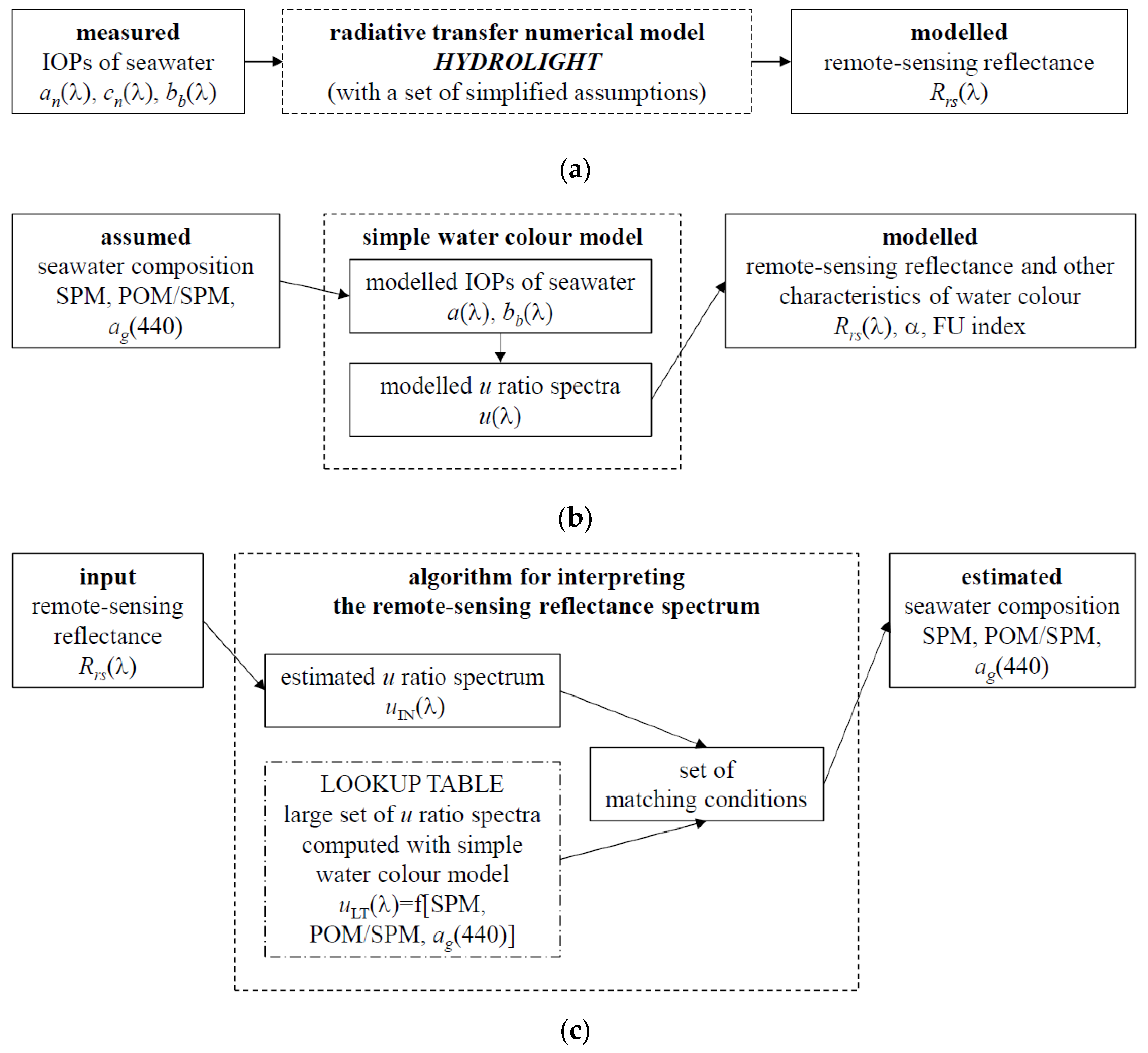
2.2. Main Modelling and Computational Approaches

In this paper, we focus on analysing potential relationships between certain biogeochemical characteristics of the seawater composition and the characteristics of its colour that can be observed remotely. One of the major parameters used in remote sensing research is the remote-sensing reflectance R_rs(λ). It is a quantity formally based on the apparent optical properties of seawater (AOPs), i.e., quantities that theoretically depend not only on the composition of seawater, but also on the lighting conditions in the atmosphere. According to the definition (see, e.g., [34]), R_rs(λ) represents the ratio of water-leaving radiance measured just above the sea surface L_w(0⁺,λ) to the downward irradiance E_d(0⁺,λ), also measured just above the sea surface. Moreover, R_rs(λ) accurately describes both the intensity of light leaving the water that can be observed under given external lighting conditions, and clearly determines what we intuitively understand by the term “water colour”. It is also known that, to a first approximation, the spectral variability of R_rs is well described by the ratio of the light backscattering coefficient to the sum of the light absorption and backscattering coefficients in water (b_b(λ)/[a(λ) + b_b(λ)]), denoted by u(λ) (the “u ratio”) (see e.g., [34,35,36]). Later in this work, we are using such approximate relationship between R_rs(λ) and u(λ).

We shall be using mathematical modelling in the later analyses and proposing practical calculation methods that use the modelling results. The modelling will entail solving the so-called forward problem, formulated as follows: How, on the basis of the composition of seawater, or its IOPs, can one estimate remotely observable spectra of R_rs and other characteristics of “colour” for light leaving the water surface? We will also put forward new algorithms for solving the so-called inverse problem, which can be stated as follows: How, on the basis of a known spectrum of R_rs (or some of its features), can one approximately estimate the composition of seawater?

Figure 1 illustrates the main models and calculation methods used in this paper. The figure consists of three simple diagrams:

• Representing the use of the standard version of the Hydrolight model to calculate R_rs spectra; such calculations are made on the basis of given (in this case measured) spectra of the absorption, attenuation and backscattering coefficients (a_n(λ) = a_p(λ) + a_g(λ), c_n(λ) and b_b(λ));
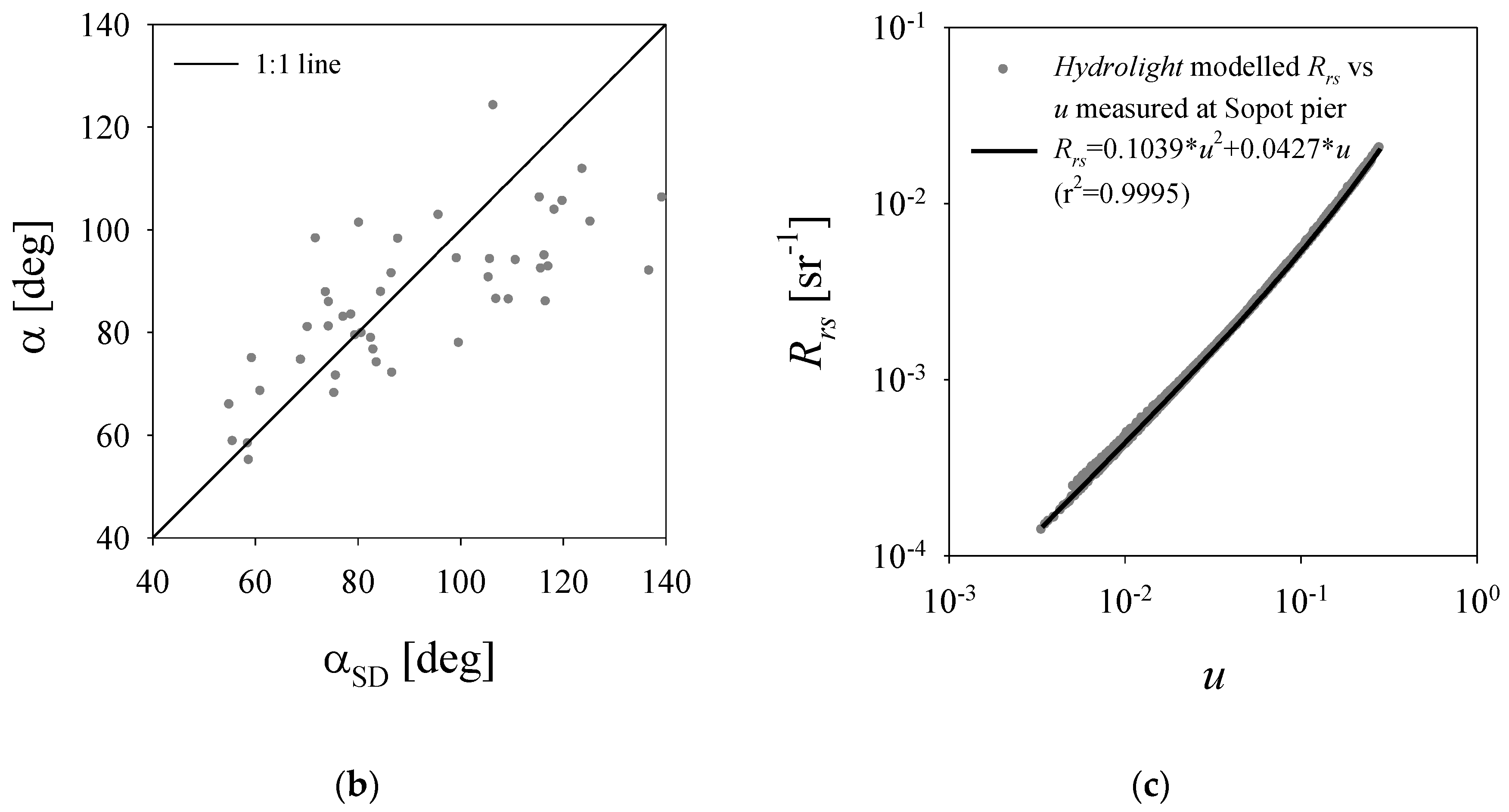
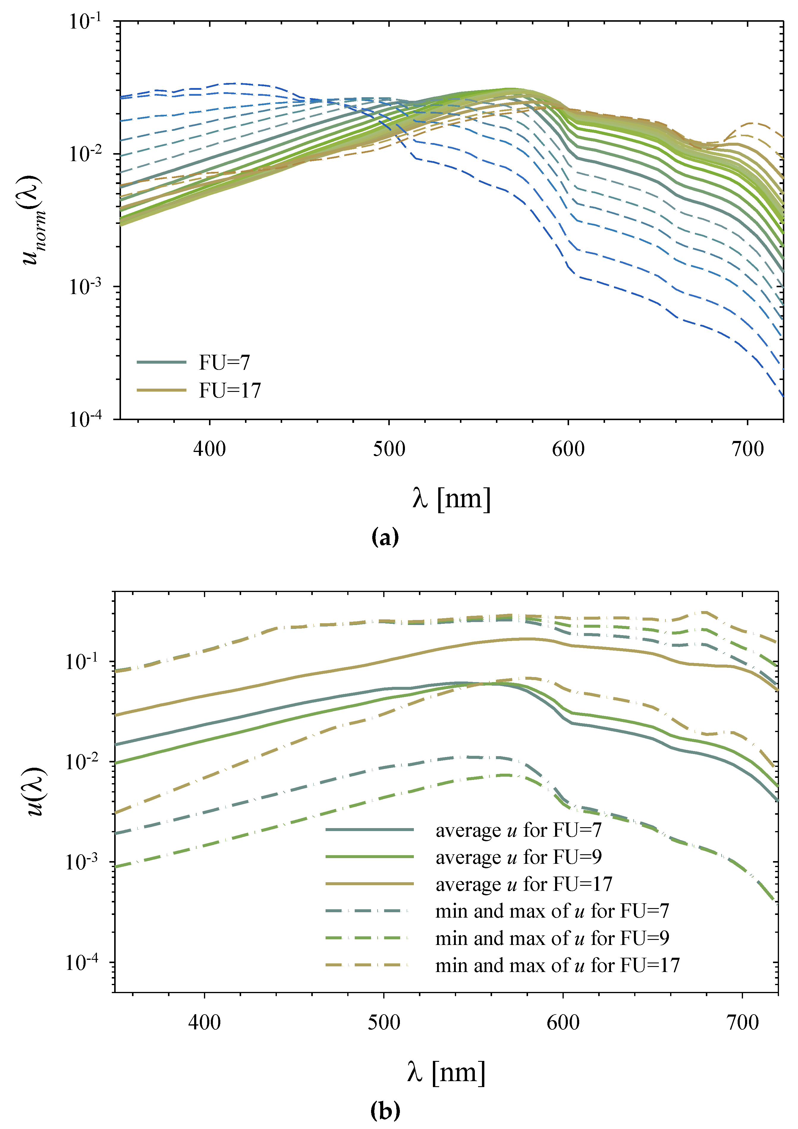
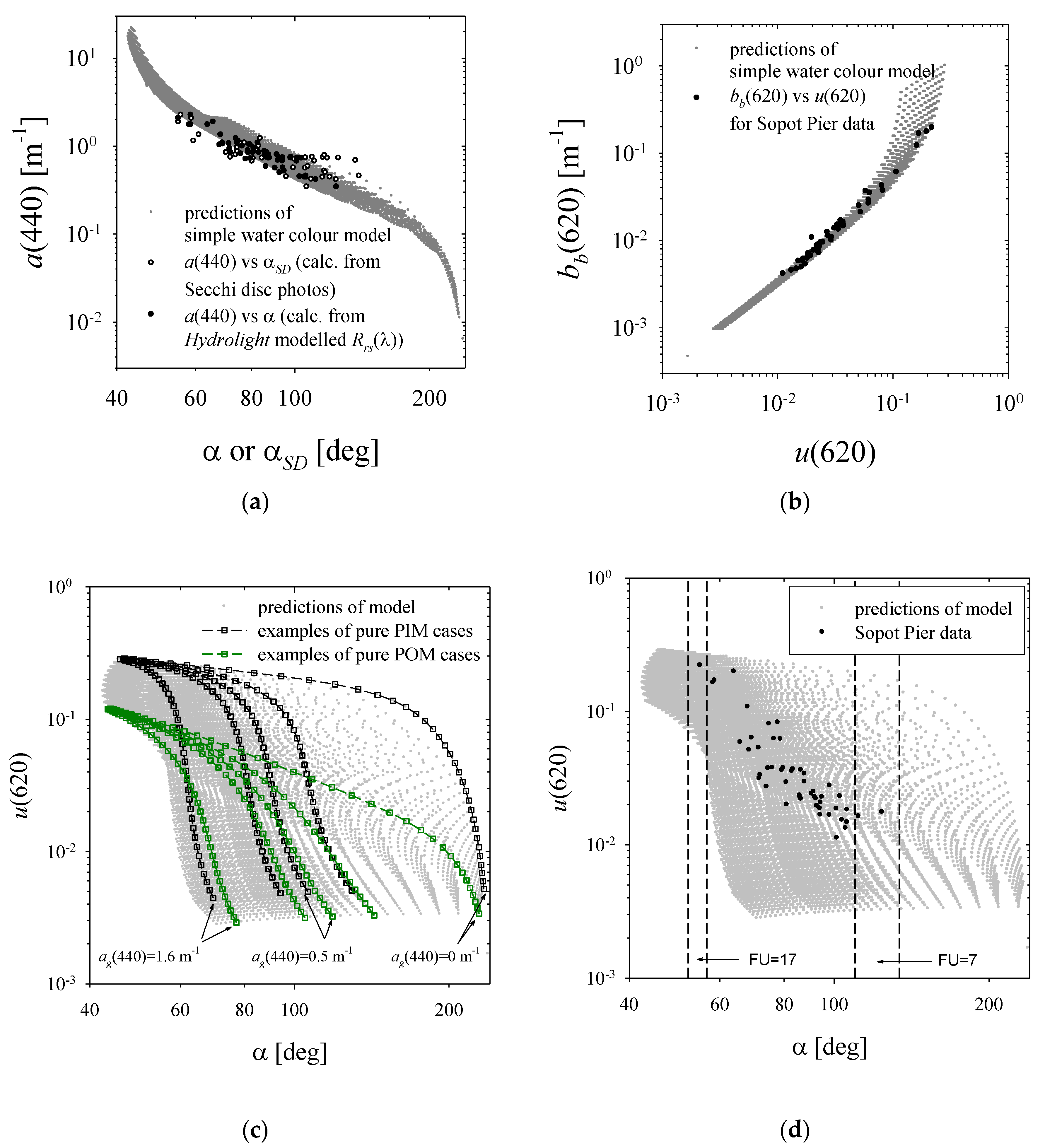
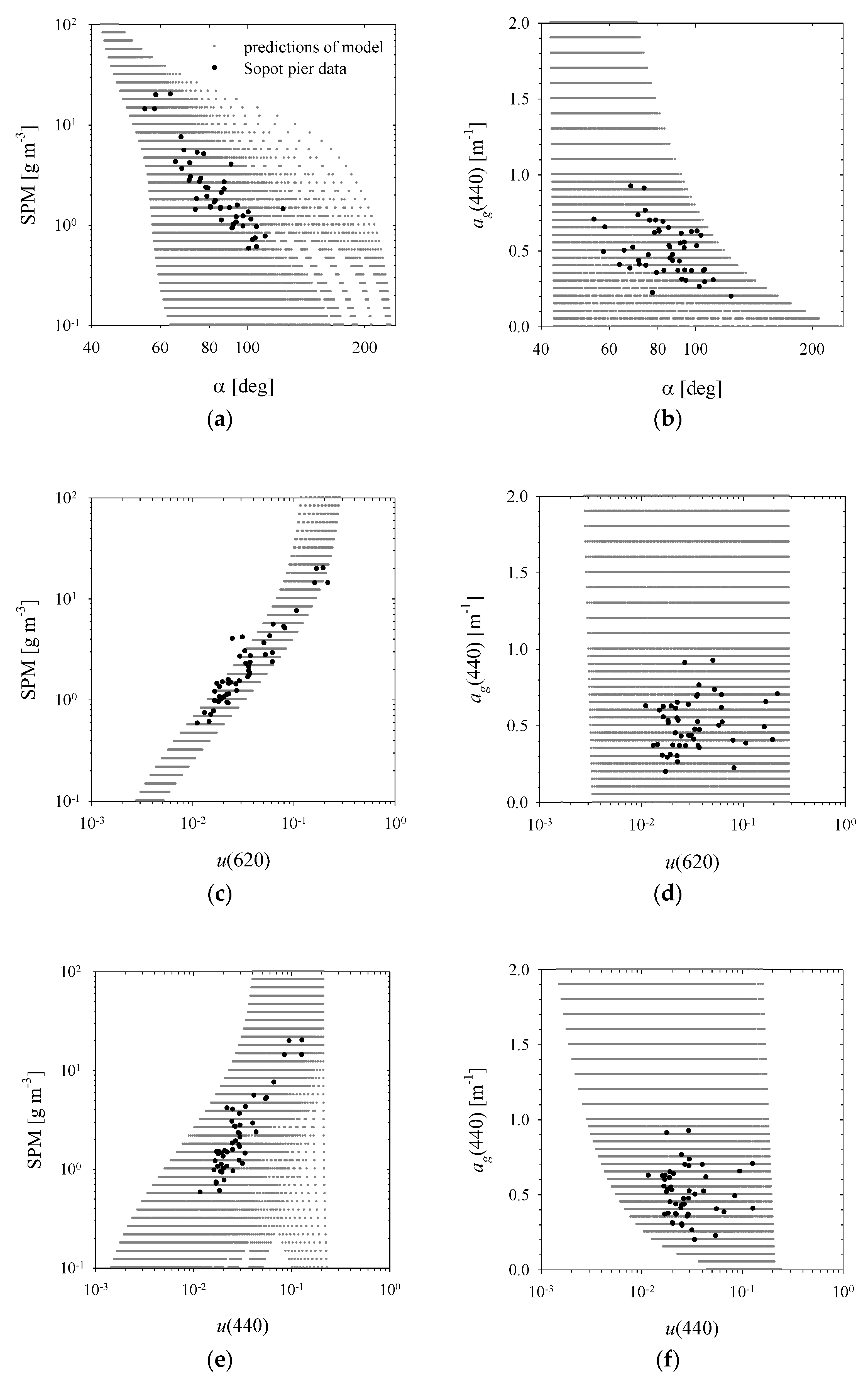
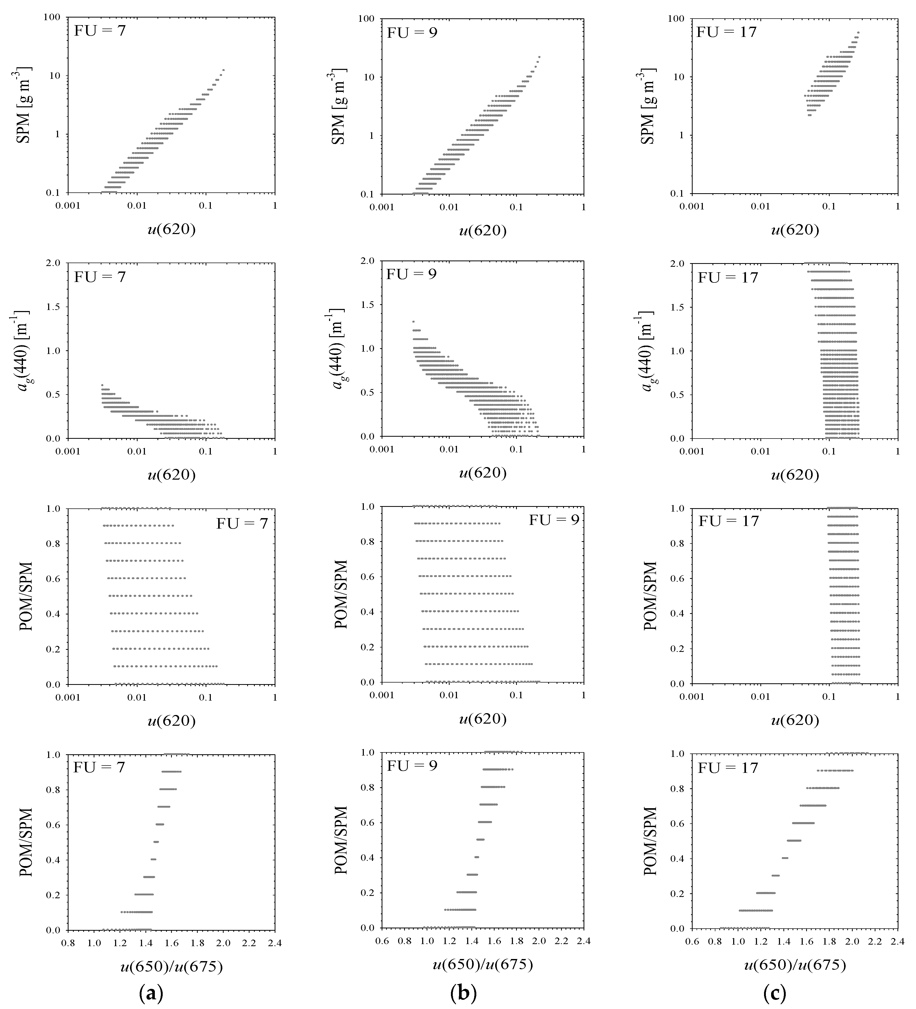
• Representing the application of a simple water colour model (a new version of the simple model proposed earlier, see [37]); with this model, for assumed values of the SPM concentration, POM/SPM and a_g(440), one can approximately determine the spectrum of R_rs, and also estimate the hue angle α and the FU index according to the Forel-Ule scale. In its intermediate steps, this model estimates the spectra of coefficients a and b_b, and calculates the spectrum of the u ratio (u(λ)), which is defined on the basis of these water IOPs;
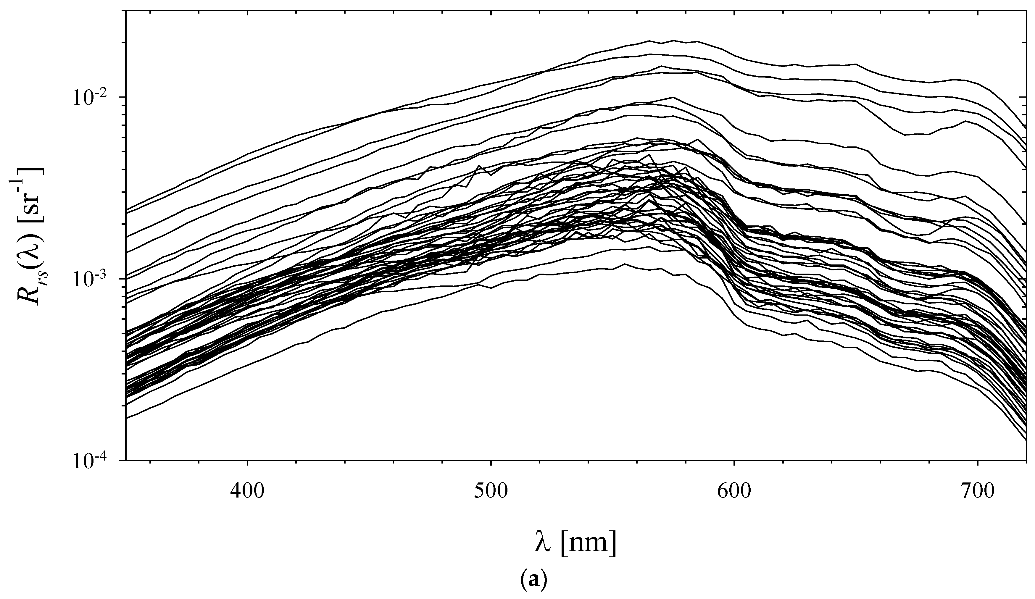
• Representing the practical algorithm for interpreting a known (input) spectrum of R_rs based on the modelling results. The new algorithms will do this as follows: On the basis of the input R_rs spectrum, the spectrum of u(λ) will first be estimated (and used as the auxiliary quantity) and then compared with the numerous spectra contained in a lookup table that pools the results obtained with the simple water colour model. Possible variants of the operation of such an algorithm will be derived by adopting alternative sets of matching conditions. Finally, the algorithm will estimate a set of values characterising the composition of seawater: SPM concentration, POM/SPM and a_g(440).

The two mathematical models mentioned above will be described in detail in the next two paragraphs, while the new algorithms resulting from the modelling will be dealt with in Results and Discussion.

2.2.1. Hydrolight Model and Simplifying Assumptions Adopted

We used version 5 of the Hydrolight radiative energy transfer model (Sequoia Scientific Inc. (Bellevue, WA, USA)). The input data for this model were the water IOPs measured during each of the 50 experiments on the Sopot pier. The calculations were performed for the 350–720 nm range with a 5 nm step. The model was supplied with the following IOPs: spectra of the absorption and attenuation coefficients by the sum of suspended and dissolved constituents, and the total backscattering coefficient (a_n, c_n and b_b, respectively). For this purpose, a_n was calculated as the sum of the measured coefficients a_p and a_g. Coefficient b_b, originally measured in only four bands in the visible range, was linearly interpolated or extrapolated over the entire 350–720 nm range. With these input data, one of the model sub-routines was able to determine the backscattering ratios and use them to select for each modelling case the approximate shape of the volume scattering function from a family of curves by Fournier and Forand (for more details, see the Hydrolight documentation [38,39]). The backscattering ratio is defined as b_b(λ)/b(λ), where b represents the (total) scattering coefficient in seawater and can be calculated from known input data as b = c − a = c_n − (a_p + a_g) + b_w, where b_w is the light scattering coefficient of pure water). When using the Hydrolight model, we also adopted a number of simplifications, similar to those we had used earlier (see [22]). In each case, a fixed solar zenith angle of 45°, cloudless lighting conditions in the atmosphere, and a minimal sea surface roughness (parameterised by a wind speed of 1 m s⁻¹) were assumed. Another simplification was that no inelastic scattering (no Raman scattering, or chlorophyll or CDOM fluorescence) or internal sources (no bioluminescence) were taken into account. It was also assumed that the seawater IOPs were constant with depth (no stratification taken into account), and that there was no influence of a bottom albedo. Carried out with such simplifying assumptions, the modelling may, of course, not always accurately reflect the conditions at the Sopot pier location. However, we made all these assumptions with the intention of performing calculations for the most ideal conditions possible, which in turn were to facilitate the study of the basic relationships between water colour characteristics and the properties and concentrations of optically important seawater constituents.

2.2.2. Simple Water Colour Model

In order to produce a large database of modelling results enabling a practical description of the relationship between the hypothetical composition of seawater and the characteristics of the water-leaving light spectrum, we decided to perform the calculations using the modified version of the “simple water colour model” that we had designed earlier [37]. One of the main assumptions of this model is that the remote-sensing reflectance R_rs, to a first approximation, can be associated with the u(λ) ratio. It also assumes that the seawater composition can be approximately described by four optically significant components: pure seawater (of the appropriate salinity), particulate organic matter (POM), particulate inorganic matter (PIM) and chromophoric dissolved organic matter (CDOM). The block diagram of this model is given in Figure 2, which also includes the main model equations/formulas.

The input data specifying the seawater composition are presented in the form of two blocks in Section I of the diagram in Figure 2. The block specifying suspended matter in water contains two quantities: the total concentration of SPM (=POM + PIM) and the ratio representing the proportion of the organic fraction in the total dry mass of particles POM/SPM. These values can, of course, be used interchangeably with POM and PIM concentrations. For the block representing CDOM, only the light absorption coefficient of these substances at the reference light wavelength of 440 nm, a_g(440), is required as input.

The main equations or sets of model formulas are presented in the form of six blocks in Section II of Figure 2. The first four blocks explicitly state equations with which the spectra of the following quantities can be calculated: total absorption and backscattering coefficients a(λ) and b_b(λ), the u(λ) ratio, and the remote-sensing reflectance R_rs(λ) (blocks II.a—II.d). Owing to the complexity of the equations, the next two blocks only symbolically represent sets of formulas for calculating the hue angle α, which characterises the water colour visible to the human eye and the relevant FU index (blocks II.e and II.f, for further details, see

Table 1. (a) Formulas for calculating the hue angle α from known spectra of R_rs (acc. to [3], see also [37]); (b) Hue angles α_FU assigned to individual classes of the Forel-Ule scale, and angles α_transition separating one class from another with a higher FU index (acc. to [3]).

(a)
$\alpha \left[\mathrm{in} \mathrm{degrees}\right]=\left(180/\pi \right)\left[\mathrm{atan}2\left(y-y_w,x-x_w\right)\mathrm{mod} 2\pi \right]$
where: - atan2 stands for a 2-argument arctangent function (for definition see Equation (3) in the main text); - xw and yw are the “white point” coordinates (which both equal 1/3); - x and y are the chromaticity coordinates:
$x=X/\left(X+Y+Z\right)$; $y=Y/\left(X+Y+Z\right)$
- X, Y and Z are the tristimulus values:
$X={{\displaystyle \int }}_{400nm}^{700nm}{R}_{rs}\left(\lambda \right)\overline{x}\left(\lambda \right)d\lambda ; Y={{\displaystyle \int }}_{400nm}^{700nm}{R}_{rs}\left(\lambda \right)\overline{y}\left(\lambda \right)d\lambda ; Z={{\displaystyle \int }}_{400nm}^{700nm}{R}_{rs}\left(\lambda \right)\overline{z}\left(\lambda \right)d\lambda$
- $\overline{x}$, $\overline{y}$ and $\overline{z}$ represent CIE 1931 colour matching functions (see text and Figure 3a).
(b)
FU Class	αFU[°]	αtransition[°]	FU Class	αFU[°]	αtransition[°]
1	229.94	227.68	12	68.49	67.93
2	225.41	219.27	13	67.36	65.98
3	213.13	205.19	14	64.6	63.35
4	197.25	189.2	15	62.11	60.37
5	181.15	165.71	16	58.26	56.64
6	150.26	133.96	17	54.65	52.09
7	117.66	109.85	18	49.53	46.75
8	102.05	95.14	19	43.96	41.82
9	88.24	83.38	20	39.67	36.98
10	78.53	74.62	21	34.28	(n. a.)
11	70.71	69.6

).

The constant values assumed in the model equations are set out in Section III of Figure 2. They are:

-

Literature values of absorption and backscattering coefficients by pure seawater, a_w(λ) and b_bw(λ). In our calculations, we used a compilation of values according to [40,41,42], as well as those from [32] (corrected for the water salinity (ca. 7) typical of the region studied);

-

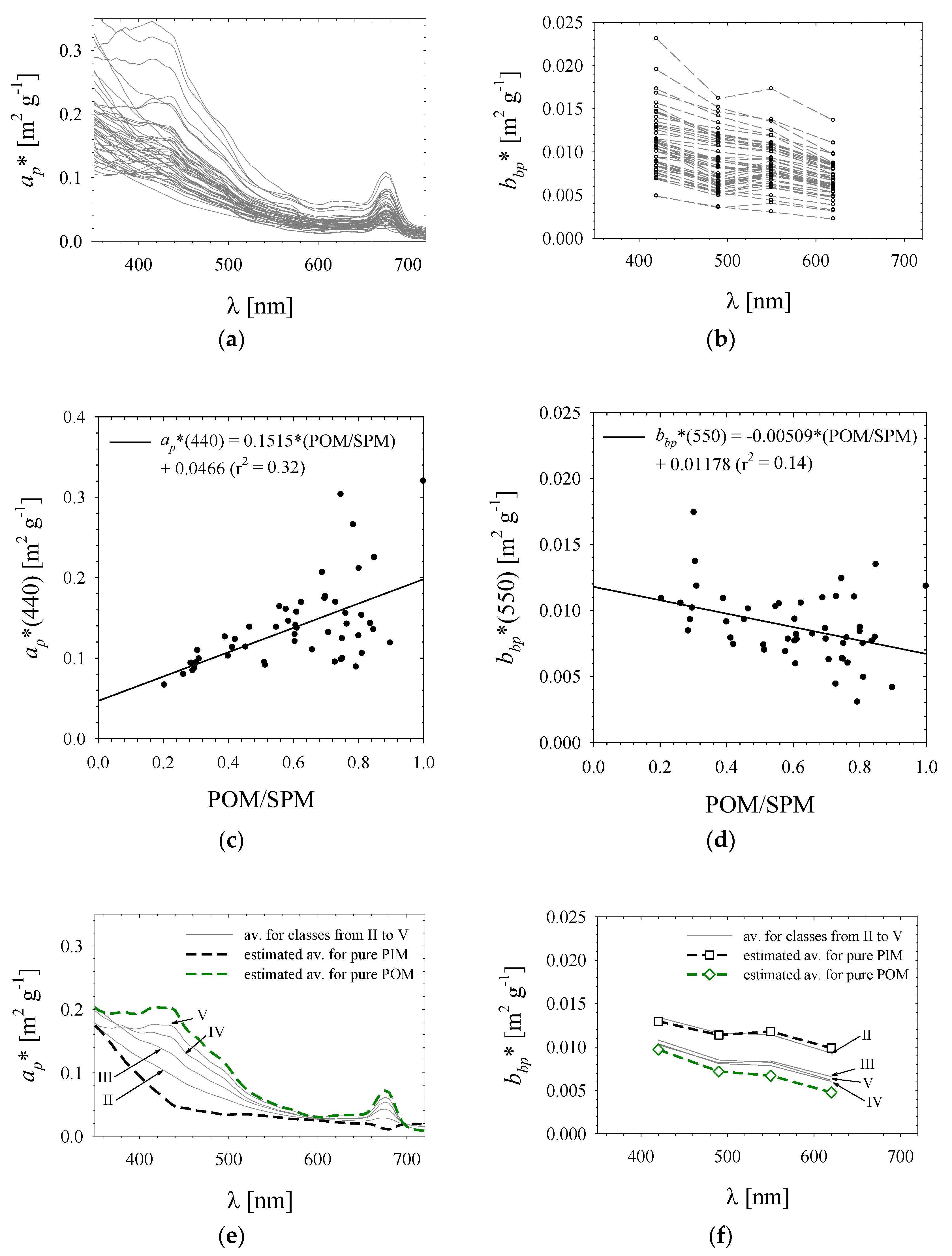
It was assumed that for both the organic and inorganic fractions of suspended particles (POM and PIM), typical/average values of the mass-specific optical coefficients could be taken into account, i.e., the coefficients respectively denoted by a_p*^POM, a_p*^PIM, b_bp*^POM or b_bp*^PIM (definitions are given later). The spectral values of these assumed constants will be determined on the basis of available empirical data and will be given in the next section;

-

It was assumed that the spectrum of the absorption coefficient by CDOM a_g(λ) could be approximated by an exponential function (the last term of the sum presented in block II.a in Figure 2), which takes into account the constant value of the typical slope of this spectrum, denoted by S_g. A typical value of this constant determined on the basis of the available empirical material will be specified in the next section;

-

It was assumed that the approximate dependence of the remote-sensing reflectance spectra R_rs(λ) on the spectra of u(λ) could be described by a quadratic function requiring only two constants, C₁ and C₂. The values of these constants, determined from the calculations done with the Hydrolight model, will be given in the next section.

Table 1 supplements the block diagram in Figure 2. It sets out detailed equations for calculating the hue angle α and the FU index based on spectra of the remote-sensing reflectance R_rs(λ). Figure 3 illustrates selected elements or dependences important for these calculations: the spectra of the colour matching functions, representing the typical sensitivity of the human eye to the colours of visible light, a graphical representation of the ranges of hue angle α for the Forel-Ule colour classes, and examples of colours that can represent these classes.

3. Results and Discussion

3.1. Variability of Biogeochemical and Optical Quantities in the Empirical Dataset

It is important to bear in mind that the biogeochemical and optical quantities in our data set, collected in the Baltic nearshore environment, are highly variable (see

Table 2. Variability of biogeochemical and optical quantities in the empirical data set.

Quantities	Average (Standard Deviation)	Minimum	5th Percentile	Median	95th Percentile	Maximum
characteristics of particulate matter
SPM [g m−3]	3.31 (4.36)	0.58	0.66	1.61	16.7	20
POM [g m−3]	1.56 (1.22)	0.35	0.36	1.15	4.26	5.18
PIM [g m−3]	1.75 (3.41)	0	0.23	0.45	12	15.9
Chla [mg m−3]	3.26 (3.43)	0.48	0.55	1.94	13.4	15.9
main characteristic of CDOM
ag(440) [m−1]	0.503 (0.164)	0.197	0.243	0.494	0.828	0.922
biogeochemical ratios
POM/SPM	0.61 (0.20)	0.2	0.28	0.62	0.87	1
Chla/POM (×10−3)	2.08 (1.06)	0.52	0.76	1.83	4.77	4.9
ag(440)/SPM [m2 g−1]	0.314 (0.221)	0.02	0.034	0.265	0.74	1.08
optical properties of particulate matter
ap(440) [m−1]	0.375 (0.36)	0.066	0.082	0.282	1.34	1.56
ap(675) [m−1]	0.128 (0.119)	0.015	0.026	0.092	0.473	0.494
bbp(420) [m−1]	0.0404 (0.0635)	0.0061	0.0071	0.0203	0.249	0.328
bbp(620) [m−1]	0.0259 (0.0426)	0.0036	0.0041	0.0105	0.169	0.193

). Some relationships between different quantities are also illustrated in Figure 4. SPM concentrations in the monitored location varied from 0.58 to 20 g m⁻³, i.e., over 30 times. The general composition of suspended matter, which can be described by the POM/SPM ratio, varied from cases with the clear dominance of inorganic particles (POM/SPM = 0.2) to cases of “pure” organic particles (POM/SPM = 1). If we divide the theoretical full range of POM/SPM variability into five equal intervals and designate them as classes from I to V (where class I represents dominance by mineral particles, with POM/SPM < 0.2, while class V represents dominance by organic particles, with POM/SPM between 0.8 and 1), we see that four of these five, theoretically separated classes, are explicitly represented in our data set (see Figure 4a). There was also significant variability within the organic particle fraction itself, which can be expressed by the ratio of the concentration of chlorophyll a to that of the organic particle fraction (Chla/POM). This ratio varied by a factor of >9 (see Figure 4c). The variability of the biogeochemical characteristics of the suspended matter meant that their IOPs also changed significantly. For the light absorption coefficients of particles a_p, the bands corresponding to the maximum light absorption by chlorophyll a (440 and 675 nm) varied by factors of 24 and 33, respectively. A more than 50-fold variation was recorded in the case of the coefficients of backscattering by particles b_bp in various bands in the visible range. Chromophoric dissolved organic matter (CDOM) also varied significantly by the Sopot pier. The a_g(440) light absorption coefficient, normally a proxy for CDOM concentration, varied widely from just under 0.2 m⁻¹ to over 0.92 m⁻¹ (a nearly 5-fold difference). As a result, the proportions between dissolved and suspended substances were extremely variable in this location; the ratio of a_g(440) to the SPM concentration varied by a factor >50 (a_g(440) to SPM relationships are also illustrated graphically in Figure 4b).

3.2. Average Specific Inherent Optical Properties—Constants for the Simple Water Colour Model

For the needs of modelling using the simple water colour model, it was necessary to determine the typical spectra of specific absorption and light backscattering coefficients by the separate organic and inorganic particle fractions. This was done as follows. First, the mass-specific optical coefficients were determined for each case—they were defined as coefficients a_p(λ) and b_bp(λ) normalised to the SPM concentration:

a_p*(λ) = a_p(λ)/SPM,

(4)

b_bp*(λ) = b_bp(λ)/SPM.

(5)

The spectra of the coefficients determined in this way for all the samples are shown in Figure 5a,b; obviously, these spectra are highly diverse. The reasons for this diversity, to a first approximation, can be seen primarily in the variety of optical properties between the organic and inorganic fractions of the matter contained in the suspended particle population. For example, some of the spectra of the coefficients a_p*(λ) exhibit clear local maxima that are most likely associated with the presence of photosynthetic pigments, while others generally take lower values and decrease almost monotonically with increasing light wavelength. Moreover, there is also a clear differentiation between the spectral values of coefficients b_bp(λ) (represented by only four wavelengths in this data set) in the individual bands.

In order to calculate the specific optical coefficients corresponding to the hypothetical “pure” organic and inorganic fractions (POM and PIM), their dependence on POM/SPM had to be approximated with linear functions using the classical least squares method for each mass-specific optical coefficient and at each wavelength of light λ_i for which data was available:

a_p*(λ_i) = C₁(λ_i) × (POM/SPM) + C₂(λ_i),

(6)

b_bp*(λ_i) = C₃(λ_i) × (POM/SPM) + C₄(λ_i).

(7)

Such linear approximations for selected spectral bands (440 and 550 nm) are exemplified in Figure 5c,d. These approximations usually have relatively low coefficients of determination r² (e.g., for a_p*(440), r² = 0.32, while the average for the whole spectral range is 0.15; for b_bp*(550), r² = 0.14, and the average for the whole spectral range is 0.13). Despite these low values of r², matching such approximations permits a rough estimate of “typical” values of mass-specific optical coefficients for the hypothetical pure organic and inorganic fractions. The spectral values of these coefficients can be written as follows:

a_p*^(POM)(λ_i) = C₁(λ_i) + C₂(λ_i),

(8)

b_bp*^(POM)(λ_i) = C₃(λ_i) + C₄(λ_i),

(9)

a_p*^(PIM)(λ_i) = C₂(λ_i),

(10)

b_bp*^(PIM)(λ_i) = C₄(λ_i).

(11)

The spectral values of the specific optical coefficients determined in this way are plotted in Figure 5e,f. With such spectra we can write approximate formulas for estimating coefficients a_p(λ) and b_bp(λ) as functions of given POM and PIM concentrations, as shown on the block diagram of the model in Figure 2 (see blocks II.a and II.b). Figure 5e,f additionally illustrate the average values of a_p*(λ) and b_bp*(λ) calculated for the proposed groups of particulate matter composition from II to V (characterised by different POM/SPM ranges). The values obtained for these four groups, especially for the light absorption coefficient, highlight the diversity of optical properties associated with the change in proportion between the organic and inorganic fractions in the total mass of particles.

In order to write a simplified model description of the spectra of the absorption coefficient by CDOM a_g(λ), the measurements of samples from the Sopot pier were approximated by an exponential function (see the last term in block II.a in Figure 2). The measured a_g(λ) spectra, normalised to the values for the reference light wavelength (440 nm), are shown in Figure 6. The calculated average coefficient S_g representing the slope of these spectra was 0.0196. This value was further used in the modelling as the typical slope of a_g(λ) spectra.

3.3. The Results of the Hydrolight Model

The remote-sensing reflectance spectra R_rs(λ), obtained with the Hydrolight model for 50 water samples from the monitored nearshore location on the Sopot pier, are shown in Figure 7a. These spectra were also further analysed in order to estimate the corresponding values of the hue angle α and the FU index (according to the formulas given in Table 1). For the set of these spectra, values of α from 55° to 124° were obtained, while the estimated FU indices varied from 7 to 17 (the median in this case was 9, and the 10th and 90th percentiles were 8 and 14, respectively). The hue angles α obtained from analyses of modelled R_rs spectra were also compared with those estimated from digital photographs of the submerged Secchi disc (α_SD) (Figure 7b). The results of these two types of estimates are only partially consistent. The differences between these values, α_SD - α, are on average 5.2° (n = 46), and the corresponding standard deviation is 15.4°. However, it should be borne in mind that here we are comparing the results of calculations performed by quite different methods, each of which is based on a different set of simplifications and probably has a great many imperfections. At this point, we would merely point out that assessments of colour based on photographs of a submerged Secchi disc may, to some extent, be burdened by an error related to the difficulty in eliminating the mirror reflection of that part of the sky situated at the zenith above the place of observation. In the case of a cloudless sky, this may lead to the appearance of an additional “blue” light component in the signal, and thus, an erroneous increase in the estimated hue angle α_SD in relation to the colour of the light actually leaving the water, originating from the reflection by the white surface of the Secchi disc.

The results obtained with the full version of the Hydrolight model were also used to determine the coefficients of the approximate quadratic relation (see block II.d in Figure 2) linking R_rs with the u ratio. This formula is plotted in Figure 7c. Coefficients C₁ and C₂ took values of 0.1039 and 0.427, respectively, and the corresponding coefficient of determination for this approximate formula was very close to unity (r² = 0.9995). The values of C₁ and C₂ were further used as constants for simplified calculations using the simple water colour model.

3.4. The Results of the Simple Water Colour Model

Calculations using the simple water colour model were carried out for the following set of input values representing the hypothetical composition of seawater:

-

37 different SPM concentrations, from 0.1 to 100 g m⁻³, obtained by using a fixed multiplier of $\sqrt[12]{10}\approx 1.212$, which yields 12 different values for each order of magnitude of variation in SPM concentration;

-

11 POM/SPM ratios, from 0 to 1, with a constant step increasing consecutive values by 0.1;

-

11 a_g(440) coefficients, from 0 to 2 m⁻¹, with a step of 0.05 m⁻¹ for values <1 m⁻¹, and a step of 0.1 m⁻¹ for values >1 m⁻¹.

Such a set of input values yielded a total of 12617 model cases of u ratio spectra corresponding to non-zero SPM concentrations. In addition, one other case was considered, corresponding to the hypothetical optically “clean” seawater (i.e., assuming SPM = 0 g m⁻³ and a_g(440) = 0 m⁻¹). All these cases formed an extensive collection of modelling results, constituting the earlier mentioned lookup table (see Supplementary Materials, Table S1).

Some examples of the modelled u ratio spectra are shown in Figure 8. These spectra represent only extreme cases of suspended matter composition, i.e., for pure POM in water (POM/SPM = 1) (right-hand panels) or only pure PIM (POM/SPM = 0) (left-hand panels). For clarity, only seven possible POM or PIM concentrations, from 0.1 to 100 g m⁻³, are shown in each panel, and only three examples of constant CDOM concentrations are considered. The upper panels correspond to the hypothetical complete lack of CDOM in water (a_g(440) = 0 m⁻¹), the middle panels are plotted for a_g(440) = 0.5 m⁻¹, which is close to the average recorded from the Sopot pier, and the lower panels are plotted for a_g(440) = 1.6 m⁻¹, which illustrate conditions typical of the waters of the Vistula, the main river flowing into the Gulf of Gdańsk. Among other things, the curves in this graph visualise the evident impact of variable POM or PIM concentrations on calculated u ratios in the red light range, and also the evident modification of the spectral shapes due to the presence of CDOM in the water, especially in the blue light range.

Associated hypothetical remote-sensing reflectance spectra R_rs (λ) were also calculated for all the modelled u ratio spectra (in accordance with block II.d in Figure 2), being subsequently used to determine the hue angle α and FU index. Figure 9a shows the average spectra of normalised u ratios for each class on the Forel-Ule scale. Normalisation was achieved by dividing the u ratios at the individual wavelengths by the integral representing the entire area under the u(λ) curve in the 350–720 nm range. When drawing the individual curves, different colours stood for the various classes (the same colours as in Figure 3c). Classes that appeared as a result of calculations using the full version of Hydrolight for the measured IOPs (i.e., classes from 7 to 17) have been highlighted. By using the simple water colour model for the assumed various hypothetical concentrations of POM, PIM and CDOM, we obtained results that could be allocated to classes 1–19. None of our modelling results corresponded to the two highest classes (20 and 21). This seems to be because we arbitrarily assumed the maximum SPM concentration to be 100 g m⁻³, and the maximum value of the a_g (440) coefficient to be 2 m⁻¹. It is likely that obtaining results from classes 20 and 21 would require even higher values for these variables.

Figure 9b represents average spectra of the u ratio obtained with the simple water colour model, along with the ranges corresponding to the maximum and minimum values of u at individual wavelengths, for three selected Forel-Ule classes (FU = 7, 9 and 17; these indices were chosen to represent minimum, median and maximum values of FU obtained from our Hydrolight model runs). The u ratio within each class can clearly be highly variable, from ca. one to even two orders of magnitude. This generally indicates that within spectra belonging to the same Forel-Ule class, one can expect very different “intensities” of water-leaving light under the same external lighting conditions (very different R_rs for particular light wavelengths). In other words, seawater seen from above the surface may have the same “colour” in the observer’s view, but at the same time may have a very different relative “brightness”.

Figure 10a,b illustrate two examples of the “strong” statistical relationships indicated by the results of calculations based on the simple water colour model. These are the relationships between selected IOPs and quantities characterising the remote-sensing reflectance spectrum. We previously reported the existence of these types of dependences in Reference [37]. Figure 10a records the relationship between the hue angle α and the total absorption coefficient of light from the blue band in seawater a(440). In general, the smaller the hue angle for the remotely observed light spectrum, the higher the total absorption coefficients of blue light in seawater. We can therefore infer that the sum of dissolved (CDOM) and suspended (SPM) components is responsible for the “colour” of water (understood as the hue angle or as belonging to the Forel-Ule classes). Taken together, these two classes of components evidently contribute to the elevated value of the absorption coefficient in the blue light band. In turn, Figure 10b records another approximate statistical relation between the u ratio and the total backscattering coefficient b_b that exists in the red light bands (e.g., for λ = 620 nm). A clear differentiation of this relationship, associated with potential changes in the suspended matter composition, manifests itself only at high values of b_b(620) and u(620). Since CDOM does not affect light backscattering and absorbs only a small amount of light in this band (compared to the large absorption coefficient of clean seawater), it has an almost negligible impact on this statistical relationship. For this reason, the remote-sensing reflectance in the red light bands can be used directly to estimate the SPM concentration (as was the case in our previous papers; see References [22,23]). Figure 10a,b also show that the data corresponding to the experiments carried out on the Sopot pier are mostly in good agreement with the relationships emerging from the modelling data obtained with the simple water colour model.

In turn, Figure 10c records the many possible combinations of α and u(620) appearing in the results of calculations carried out with the simple water colour model (see the grey points on this graph). This figure also exemplifies curves that illustrate changes in the relevant quantities, assuming a constant CDOM concentration, and at the same time, varying concentrations of either pure POM or pure PIM. These curves show that waters of different composition, containing either pure POM or pure PIM, may appear to have the same hue angle α. However, when there are both medium and high concentrations of suspended particles, regardless of the same hue angle, there are significant differences in the levels achieved by u(620). Intuitively, higher values of u(620) (and therefore higher values of R_rs(620), and hence the greater “brightness” observed in the red light band) should be expected for particles of mineral origin, which are responsible for strong light backscattering in water. Moreover, obviously, lower values of u(620) should be generally expected for pure organic particles. Another aspect illustrated by this diagram is that even at very low SPM concentrations (the lowest points in the diagram represent POM or PIM concentrations of 0.1 g m⁻³), the presence of CDOM in water precludes high hue angles α. For example, assuming a_g(440) = 0.3 m⁻¹ and a low POM or PIM concentration of 0.1 g m⁻³, α predicted by the model will be no greater than 129° or 143°, which corresponds to classes 7 or 6 on the Forel-Ule scale.

Figure 10d is a diagram resembling that in Figure 10c, but it also shows the location of points corresponding to the data measured from the Sopot pier. As a background to this figure, the same grey points as in Figure 10c are used, obtained from using the simple water colour model for hypothetical seawater compositions. This diagram shows that with the aid of simplified modelling, we can cover a much larger range of hypothetically possible water compositions than what we managed to record on the Sopot pier, and which we used to calibrate the constants used in the simple water colour model.

Figure 11 illustrates the direct relations between the main quantities characterising the possible composition of seawater and selected characteristics of water-leaving light resulting from the modelling. The ranges of SPM concentrations or CDOM absorption coefficients a_g(440) can be determined from some of the diagrams in this figure, depending on the colour represented by the hue angle α, or the known intensity of the signal in the red and blue bands given by the respective values of u(620) and u(440). Among other things, the figure shows that the upper limit of possible SPM concentrations can be estimated from a known hue angle α (Figure 11a), and in cases where α takes high values, also the upper limit of a_g(440) (Figure 11b). It shows, moreover, that from a known value of u(620), one can estimate the upper and lower limits of possible SPM concentrations (Figure 11c). In addition, for some ranges, one can estimate the upper limit of possible SPM concentrations from known u(440) (Figure 11e), and, at the same time, the lower limit of a_g(440) (Figure 11f).

Using the relationships involving the hue angle α shown in Figure 10a and Figure 11a,b, one can produce a summary table for quantitatively interpreting the Forel-Ule colour classes (see

Table 3. Limits of different quantities in the Forel-Ule classes estimated using the simple water colour model: the lower and upper limits of the total absorption coefficient a(440) for each class; the upper limit of the SPM concentration (also the upper limit of the PIM concentration) for each class; the upper limits of POM concentrations for each class.

FU Class	Minimum of a(440) [m−1]	Maximum of a(440) [m−1]	Maximum of SPM (Maximum of PIM) [g m−3]	Maximum of POM [g m−3]
1	0.011	0.0267	0.261	0.1
2	0.0211	0.049	0.562	0.215
3	0.0381	0.0822	1.21	0.383
4	0.0646	0.13	2.61	0.562
5	0.0948	0.223	4.64	0.9
6	0.133	0.391	8.25	1.47
7	0.224	0.626	12.1	2.15
8	0.338	0.926	14.7	3.16
9	0.488	1.33	21.5	4.64
10	0.689	1.73	26.1	5.62
11	0.952	2.03	26.1	6.81
12	1.15	2.04	26.1	8.25
13	1.24	2.07	31.6	8.25
14	1.34	2.14	31.6	10
15	1.52	2.51	38.3	12.1
16	1.75	3.16	46.4	14.7
17	2.09	4.62	56.2	21.5
18	2.84	>9.45	>100	46.4
19	5.07	>21.8	>100	>100

). For individual classes, this table sets limits of various quantities predicted by the model: the upper and lower limits of the total absorption coefficient a(440), the upper limit of the SPM concentration (which is also the upper limit of the PIM concentration) and the upper limit of the POM fraction in water. These limits are set for classes 1–19, i.e., those that we recorded as a result of the modelling. However, it should be borne in mind that the maximum value of a_g(440) used in the modelling was 2 m⁻¹ and the maximum SPM concentration was 100 g m⁻³. Therefore, some estimated upper limits, such as those obtained for classes 18 and 19, may not represent the actual full range corresponding to such classes. However, in the case of the other classes (1–17), we can expect the estimated limits to have been correctly calculated within the range of accuracy obtainable by adopting discrete values of the SPM concentration and a_g(440) in the modelling.

On the basis of the modelling results presented so far, one can suggest a possible order of steps in the practical interpretation of known/measured spectra remote-sensing reflectances. One can combine the information carried by the water colour (hue angle α) with information carried by the signal intensity in the red band (expressed by u(620)). This is illustrated by the examples in Figure 12, plotted for three FU classes (7, 9, 17). They indicate that, after having determined the membership of a spectrum in a particular colour class, taking the value of u(620) into account may enable the ranges of both the SPM concentration and a_g(440) in the water to be estimated. Unfortunately, however, the modelling results also indicate that combining these two types of information (α and u(620)) in most cases does not give the specific proportions between the organic and inorganic fractions of suspended matter (see the third row of graphs in Figure 12 recording the relationship POM/SPM vs. u(620)). Analysing the modelling results in greater detail, we noticed that we could draw partial inferences about the composition of suspended matter based on the shape of the u ratio spectrum in the 650–675 nm range; this is illustrated by the last row of graphs in Figure 12 showing the relationships of POM/SPM vs. u(650)/u(675). However, this suggestion should be treated with particular caution, because we are aware that the simple water colour model may not accurately reflect the value at these wavelengths. In this spectral range, the influence of phytoplankton fluorescence, which our simple model does not take into account, may affect the details of the spectrum’s shape.

The relationships and interdependences presented so far, revealed by the results of the simple water colour model calculations, will be used in the next paragraph to formulate examples of algorithms that we believe can be used in practice to interpret the remote-sensing reflectance R_rs(λ) spectra in optically complex marine environments.

3.5. Examples of Algorithms for Estimating the Composition of Seawater Using the Modelling Results

At this point, it is important to recall that we want to use the modelling results corresponding to the solution of the so-called forward problem in order to develop and preliminarily test the effectiveness of practical algorithms for estimating the composition of seawater, which is essentially solving the so-called inverse problem. As an important aspect of these new algorithms, we want to use the numerous data on the u(λ) ratio spectra obtained with the simple water colour model. We assume that such data can provide an approximate description of the complex relationship between the composition of water and the properties of the water-leaving light spectrum, which can be observed remotely. In addition to the possibility of formulating such algorithms alone, it seems advisable to perform preliminary tests of their accuracy. Unfortunately, we do not have directly measured spectra of R_rs for the monitored location on the Sopot pier. Nevertheless, in order to conduct a preliminary test of the operation of the new algorithms (which, of course, should not be confused with their full and formal validation), we propose to use the R_rs spectra obtained with the full version of the Hydrolight model. Note that, unlike the simple water colour model, which was based on the assumed average values of the specific optical properties of seawater components, and assumed different hypothetical concentrations of these components, the Hydrolight model did not use information about the composition of seawater in any way, but only took into account the spectra of seawater IOPs that were actually measured for each of the 50 cases analysed. Therefore, later in this paper, the R_rs spectra obtained with the Hydrolight model (shown earlier in Figure 7a) will be treated as “input spectra” that will replace the “real spectra” of R_rs.

Using the results given in the previous paragraph as potential “hints” as to how to quantify the “input spectra” of R_rs, several different approaches to the formulation of practical algorithms were tested. In each case, the first calculation step was always to estimate the u ratio spectrum, which corresponds to the R_rs “input spectrum” (this spectrum is denoted by u_IN(λ); see diagram c in Figure 1). Next, this estimated spectrum was compared with the spectra from the lookup table (Table S1) denoted by u_LT(λ). Various criteria were regarded as matching conditions. We attempted to find the best match of one full spectrum of quantity u(λ) using all the available spectral information, and we also sought entire subsets of “similar” spectra using various combinations of criteria related to certain features of the spectra. Tested, among other things, were the following criteria: membership of the sought-after spectra in the same Forel-Ule class; having similar u ratios in the red band (similar u(620)); having similar values of the ratio u(650)/u(675), or having similar tristimulus values X, Y and Z (which are intermediate quantities calculated using colour matching functions when estimating the hue angle α; see the relevant formulas given in Table 2).

Below, we discuss in detail just two variants of the algorithm we tested, i.e., those that offered the best accuracy when we were attempting to evaluate the composition of seawater based on R_rs spectra.

The first algorithm (referred to as Algorithm I) uses all the available spectral information. It involves finding in the lookup table (Table S1) one specific spectrum of u_LT that seems to be the closest to the analysed u_IN spectrum, then retrieving the relevant values of SPM, POM/SPM and a_g(440) on the basis of which the chosen spectrum u_LT was generated. The closest spectrum from the lookup table is selected by finding the minimum for the quantity called error_score:

error_score = mod(<err_i>) + SD(err_i),

(12)

where the first term in the sum represents the absolute value of the mean calculated over the all analysed light wavelengths λ_i for the quantity err_i = u_IN(λ_i) − u_LT(λ_i), while the second term represents the standard deviation of err_i.

The second algorithm (referred to as Algorithm II) uses only a selection of the available spectral information. This algorithm matches the whole subset of the u_LT spectra to the u_IN spectrum so that these spectra have the same FU index, i.e., belong to the same Forel-Ule class, and that the values in the red band (u_IN(620) and u_LT(620)) do not differ by more than ±5%. As an estimate of the seawater composition, this algorithm gives average values of SPM, POM/SPM and a_g(440) calculated for a subset of solutions selected from the lookup table.

The diagram in Figure 10d highlights the complexity of the selection of spectra from the lookup table. There are ambiguities in this process; in some respects, many model spectra often seem similar to the “input” spectrum being analysed. Hence, the tendency to increase the number of different matching criteria seems natural. In accordance with this concept, we tested several variants of algorithms similar to Algorithm II, but using more criteria relating to certain spectral characteristics of the reflectance R_rs(λ). However, the results yielded by these more complex algorithms turned out to be less accurate. Algorithm II uses only the water colour estimated by the human eye and the intensity of the signal recorded in the red band. One can only assume that the major factors preventing the determination of better functioning algorithms using a greater number of matching conditions include the discrete nature of the lookup table (it contains a large but nonetheless finite number of cases) and the generally very approximate nature of the modelling procedure itself.

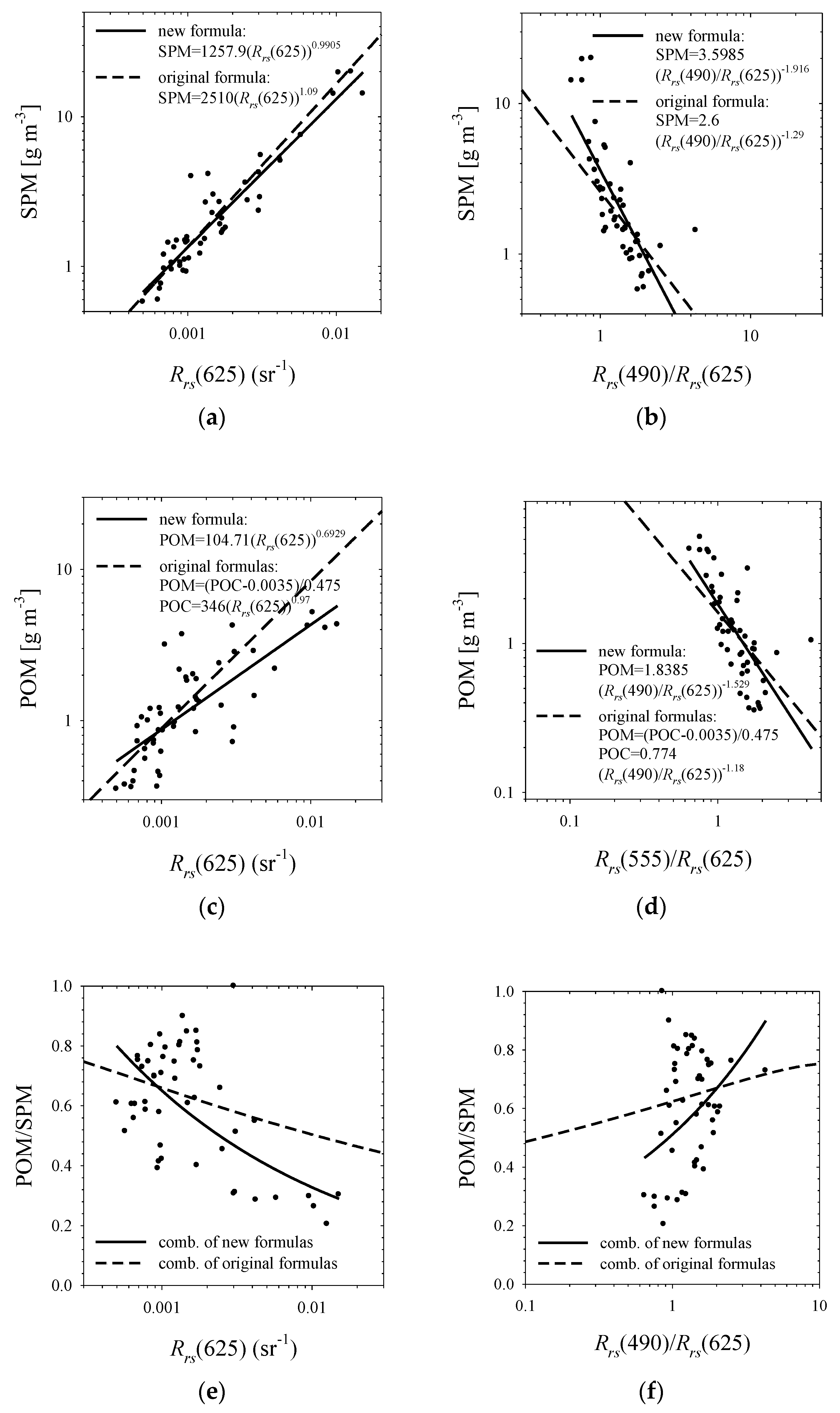
3.6. Existing Simple Statistical Formulas for Estimating Seawater Composition and Their Modified Versions Adapted to the Current Dataset

Before we pre-assess the accuracy of the seawater composition estimated with Algorithms I and II, we will examine, for comparison, some sets of much simpler statistical formulas, which could be employed for the same purpose. We will refer here to our earlier formulas that we derived from field measurements carried out in various regions of the Baltic Sea. In our earlier work [23], we included simple formulas for estimating SPM and particulate organic carbon (POC) concentrations as a function of the remote-sensing reflectance in the 625 nm band, or as a function of simple reflectance ratios (“colour ratios”) in two bands, e.g., the blue and the red (490 and 625 nm). Moreover, using the approximate relationship between POM and POC concentrations that we derived for Baltic conditions (see Reference [21]), one can use these simple statistical formulas to estimate both the total suspended particulate matter concentration (SPM) and the concentrations of the POM and PIM fractions (where POM can be calculated as a function of the POC concentration, while PIM can be calculated as the difference between estimated SPM and POM concentrations). The results obtainable with these original formulas, as well as the results acquired with the newly derived but similar formulas using the same variables but properly matched numerical coefficients, are presented in Figure 13 (the relevant equations are given in the panels). The coefficients of the new versions of the formulas were obtained by means of linear least square regression between the logarithms of the dependent variables (either SPM or POM) and the logarithms of the independent variables (either R_rs(625) or R_rs(490)/R_rs(625)).

3.7. Comparison of the Accuracies of Estimation Using the New Algorithms and the Simple Statistical Formulas

The accuracies of estimation obtained using Algorithms I and II and the new version of the simple statistical formulas (which are functions of only R_rs(625) or only the ratio of R_rs(490)/R_rs(625)) are compared in Figure 14 and

Table 4. Comparison of retrieved and measured quantities (SPM, POM and PIM concentrations, POM/SPM, and a_g(440)) with different variants of the new algorithms or sets of simple statistical formulas (Algorithms I, II, the set of statistical formulas using R_rs(625) only, and the set of formulas using only the ratio R_rs(490)/R_rs(625)). The values characterising the arithmetic statistics of the absolute and relative errors, and the logarithmic statistics are given. The definitions of the quantities used are given in the footnotes to the table.

Quantity	n	Arithmetic Statistics of Absolute Error *		Arithmetic Statistics of Relative Error **		Logarithmic Statistics ***
		MB	RMSE	MNB [%]	RMSNE [%]	log.sys.err. [%]	X
Algorithm I
SPM	49	0.36 g m−3	1.53 g m−3	4.3	28.2	0.2	1.35
POM	49	0.27 g m−3	0.91 g m−3	30.6	64.6	13.5	1.79
PIM	49	0.10 g m−3	1.13 g m−3	−1.0	160.1	−38.7	2.50
POM/SPM	50	0.11	0.23	21.5	42.8	13.3	1.50
ag(440)	49	0.06 m−1	0.17 m−1	16.4	38.8	11.4	1.33
Algorithm II
SPM	49	−0.48 g m−3	0.99 g m−3	−16.7	22.3	−19.9	1.34
POM	49	−0.53 g m−3	0.83 g m−3	−26.0	41.3	−35.3	1.70
PIM	49	0.06 g m−3	0.53 g m−3	24.2	57.5	13.7	1.51
POM/SPM	50	−0.12	0.16	−14.5	28.1	−19.2	1.43
ag(440)	49	0.08 m−1	0.18 m−1	20.8	41.7	14.3	1.40
functions of Rrs(625)
SPM	49	−0.26 g m−3	1.22 g m−3	3.3	27.1	−0.7	1.34
POM	49	−0.15 g m−3	0.77 g m−3	10.7	51.5	−0.6	1.62
PIM	49	−0.11 g m−3	1.11 g m−3	24.8	69.7	10.7	1.61
POM/SPM	50	−0.02	0.18	4.5	30.8	0.1	1.35
functions of Rrs(490)/Rrs(625)
SPM	49	−0.68 g m−3	3.25 g m−3	13.8	47.3	1.1	1.74
POM	49	−0.20 g m−3	0.78 g m−3	13.2	52.8	0.4	1.69
PIM	49	−0.48 g m−3	2.80 g m−3	60.6	119.0	17.9	2.44
POM/SPM	50	−0.04	0.19	6.0	40.9	−0.7	1.43

* arithmetic statistics of absolute error (bias): ${\epsilon }_a=P_i-O_i$ (where P_i—predicted value, O_i—observed value); mean bias: $\mathrm{MB}=\langle {\epsilon }_a\rangle =\frac{1}{n}{{\displaystyle \sum }}_{i=1}^n{\epsilon }_a$; root-mean-square-error: $\mathrm{RMSE}={\sigma }_{\epsilon a}={\left[\frac{1}{n-1}{{\displaystyle \sum }}_{i=1}^n{({\epsilon }_a-\langle {\epsilon }_a\rangle )}^2\right]}^{\frac{1}{2}}$; ** arithmetic statistics of relative error (normalised bias): ${\epsilon }_r=\frac{P_i-O_i}{O_i}$; mean normalised bias: $\mathrm{MNB}=\langle {\epsilon }_r\rangle =\frac{1}{n}{{\displaystyle \sum }}_{i=1}^n{\epsilon }_r$; root-mean-square-normalised-error: $\mathrm{RMSNE}={\sigma }_{\epsilon r}={\left[\frac{1}{n-1}{{\displaystyle \sum }}_{i=1}^n{({\epsilon }_r-\langle {\epsilon }_r\rangle )}^2\right]}^{\frac{1}{2}}$; *** logarithmic statistics (statistics calculated on logarithmic error: ${\epsilon }_{log}=\log \left(\frac{P_i}{O_i}\right)$); logarithmic systematic error: $log.sys.err.={10}^{\langle {\epsilon }_{log}\rangle }$, where $\langle {\epsilon }_{log}\rangle =\frac{1}{n}{{\displaystyle \sum }}_{i=1}^n{\epsilon }_{log}$; standard error factor: $\mathrm{X}={10}^{{\sigma }_{log}}$, where ${\sigma }_{log}={\left[\frac{1}{n-1}{{\displaystyle \sum }}_{i=1}^n{({\epsilon }_{log}-\langle {\epsilon }_{log}\rangle )}^2\right]}^{\frac{1}{2}};$ X allows to calculate a range of statistical error according to the logarithmic statistics; this range is from σ₋ to σ₊, where: ${\sigma }_{-}=\frac{1}{\mathrm{X}}-1$ and ${\sigma }_{+}=\mathrm{X}-1$.

. The table lists the classical “arithmetic” statistics of both absolute and relative errors, as well as the “logarithmic” statistics (the relevant formulas are given in the footnotes to the table). Here, we point out that the commonly used “arithmetic” statistics appear sufficient to describe the accuracy of estimating quantities that vary only slightly (such as POM/SPM, or a_g(440), which in our empirical data set varied only ca. 5-fold). Where quantities vary to a much greater extent, as with SPM, POM and POC concentrations, which differ by a factor of 50 or more in our data set, it seems more appropriate to use “logarithmic” statistics.

The calculations indicate that for estimating the SPM concentration, Algorithm I is as accurate as the simple statistical formula using only reflectance in the red band (R_rs(625)). In both cases, the systematic error according to logarithmic statistics (log.sys.err.) is close to 0%, whereas the statistical error, given the standard error factor X, is in these two cases of the order of X = 1.35 (here, X corresponds to the statistical error limits from σ₋ = −26% to σ₊ = 35%; see the formulas given in the footnote to Table 4). In the case of Algorithm II, which, when searching for solutions, takes into account only u(620) values and the hue angle α calculated from the shape of the whole input R_rs spectrum, we see that its application is encumbered by a similar statistical error (standard error factor X = 1.34) but also by a significant systematic error (log.sys.err.) of ca −20%. The accuracy of estimation of the SPM concentration seems to be the lowest with the simple formula using the ratio R_rs(490)/R_rs(625). Here, admittedly, the systematic error (log.sys.err.) is negligible (ca 1%), but the statistical error can be described by a much larger standard error factor X of 1.74. In the case of “ideally” estimated values of the quantity tested (in an error-free case), logarithmic statistics should show a systematic error (log.sys.err.) of 0% and a standard error factor (X) of 1.

For the POM concentration, a greater accuracy than with Algorithms I, II seems obtainable using simple statistical formulas with appropriately adjusted coefficients. This applies to both the relationship using the value of R_rs(625) alone and the one that uses R_rs(490)/R_rs(625). The systematic errors of these specially matched simple statistical formulas are negligibly small (log.sys.err. < 1%); this is obviously because we are testing the operation of these formulas on the same data on the basis of which their coefficients were determined. When Algorithms I and II are applied, the systematic errors (log.sys.err.) are much worse—ca +14% and −35%, respectively. More importantly, however, comparison of the standard error factors shows that these are slightly better for the simple statistical formulas (X = 1.62 or 1.69) than for Algorithms I and II (X = 1.79 and 1.70, respectively). In addition, the quantities describing the error levels for POM estimates, regardless of which variant of the new algorithm or simple formula is used, are generally higher than when estimating the total SPM concentration.

For estimates of the PIM concentration, the results are slightly different. Here, Algorithm II seems to offer the best accuracy of all the variants analysed: the systematic error (log.sys.err.) is relatively low (ca 14%) and the standard error factor (X) takes the lowest value of 1.51.

The quality assessment of the suspended matter composition present in water can also be assessed in a slightly different way, namely, by analysing the accuracy statistics of estimating the POM/SPM ratio. In this case, classical arithmetic statistics of the absolute error appear to be the most appropriate. Looking at the values given by this type of statistics, one can generally say that they are similar for the variants under consideration, with the simple statistical formulas offering only slightly better values than the new Algorithms I, II. Although the root mean square errors (RMSE) do not drastically differ (generally they vary from 0.16 to 0.23 between the worst and best cases), the mean biases (MB) are slightly more favourable for simple formulas (they are −0.02 or −0.04 for simple formulas, compared to 0.11 and −0.12 for Algorithms I, II).

The last quantity, the accuracy of estimation of which is outlined in Table 4, is a_g(440). The estimation errors in this case are shown only for the new Algorithms I and II which, by analysing the characteristics of the entire “input spectra” of the reflectance R_rs(λ), can also estimate this additional quantity. Both new algorithms have a noticeable systematic error (mean bias (MB)) of 0.06 or 0.08 m⁻¹, as well as a statistical error (root mean square error (RMSE)) of 0.17 or 0.18 m⁻¹.

At this point, we should emphasise that the simple statistical formulas, which utilise only the red reflectance or just one simple “colour ratio”, were specially derived by matching their coefficients to the now available data set. The fact that these coefficients differ significantly from the prototypes of these formulas (compare the equations in Figure 13a–d) most likely means that they do not have the potential to be universal formulas, that is, they will probably not work well for input data from outside the set for which they were developed. In our opinion, the existence of these simple formulas appears to indicate which part of the information contained in the spectrum of R_rs may be the most important for estimating biogeochemical quantities characterising seawater composition. However, we consider that the potential value of the new, much more complex Algorithms I, II lies in the fact that they attempt to simultaneously use information about both the reflectance in the red and the water colour assessed on the basis of the shape of the entire R_rs spectrum (not only two particular, narrow spectral bands). It also seems important that these algorithms simultaneously estimate not only the quantities characterising the levels of suspended particle matter in seawater (SPM, POM and PIM concentrations), but also the amount of CDOM in water. It seems that our new algorithms have the potential to be the basis for practical methods with a much greater range of applicability and greater versatility than the specially adapted simple statistical formulas we have been discussing. For the time being, of course, this is merely an intuitive statement, which will have to be assessed by conducting a formal validation of all the methods discussed here, based on an independent empirical data set.

4. Summary and Conclusions

Simplified mathematical modelling was used to illustrate and analyse the complex relationships between the seawater composition in the nearshore environment of the Baltic Sea and various remotely observable water colour characteristics. These characteristics included the spectra of both the remote-sensing reflectance R_rs(λ) and the u ratio, i.e., the ratio of the backscattering coefficient to the sum of the absorption and backscattering coefficients (b_b/(a + b_b)); the latter ratio is closely related to R_rs(λ), defined only by the inherent optical properties (IOPs) of seawater. The quantities associated with the perception of water colour by the human eye were also analysed; the hue angle α and the FU index representing different classes according to the traditional Forel-Ule water colour scale.

We based this study on empirical data obtained from regular experiments in a nearshore location (the Sopot pier) on the coast of the Gulf of Gdansk, in the southern Baltic Sea. These data were used, inter alia, for calibrating a simple water colour model linking seawater composition with certain characteristics of water-leaving light.

With the aid of modelling, we achieved both our objectives, above all, the main one, which was to demonstrate the probable complexity of the relationships between the biogeochemical characteristics of suspended and dissolved substances in seawater and the remotely-sensed characteristics of light. To achieve this goal, we presented analyses of possible variations of the u ratio spectra (see Figure 8), from which one can draw inferences about the expected variability in the spectra of the remote-sensing reflectance R_rs. The traditional Forel-Ule colour scale was also interpreted quantitatively; typical shapes of normalized u ratio spectra assigned to individual FU classes were illustrated (see Figure 9). The estimated limits of the total light absorption coefficient in the blue band (a(440)) as well as the upper limits for the concentrations of (total) suspended particulate matter (SPM) and their POM and PIM fractions that can be expected within the individual classes were given (see Table 3).

The additional objective was also achieved, namely, the derivation of examples of practical algorithms applicable in remote sensing studies. With the aid of a wide range of modelling results set out in a lookup table (Table S1), based on a given spectrum of R_rs or some of its features, the approximate composition of seawater can be estimated with these algorithms. This composition is determined by estimating the total concentration of suspended particulate matter (SPM), the proportion of the organic fraction (POM/SPM), and a proxy characterising the CDOM concentration, i.e., the light absorption coefficient of these substances in the blue band (a_g(440)).

These new algorithms more or less directly use information contained in the entire remote-sensing reflectance spectrum, not just in particular spectral bands. Algorithm I compares the entire u ratio spectrum corresponding to the R_rs spectrum with the tabulated modelling results. Algorithm II is based on the most significant features of R_rs, i.e., the combination of information about the hue angle α (calculated from the shape of the entire R_rs spectrum) with information on the intensity of light in the red part of the spectrum (where the effect of suspended matter in seawater is most clearly manifested).

The accuracy with which these two algorithms match the individual measurements made in the nearshore environment of the Baltic Sea was assessed statistically. Note that this was merely a preliminary assessment of this accuracy, not a validation, which, of course, will need to be performed on an independent data set. Our initial assessment indicates that in some cases the accuracy of the new algorithms in relation to the estimation of quantities characterising suspended matter in water (SPM, POM and PIM) may be slightly better, and in other cases, slightly worse than the accuracy of simple, “locally” calibrated empirical formulas, i.e., those using only certain information carried by the R_rs spectrum. Nevertheless, we can put forward the following arguments in support of the potential of the new algorithms. Firstly, besides characterising suspended matter, they simultaneously estimate the proportion of CDOM in seawater. Secondly, the assumption adopted in the modelling, that the composition of suspended matter and its proportions relative to the presence of CDOM are not correlated in any way, at least allows one to expect that these algorithms may have a more universal application than simple statistical formulas with “locally” matched coefficients. Obviously, this statement will require confirmation based on an independent data set.

Finally, we consider that the results and analyses presented in this paper may be significant not only for the nearshore regions of the southern Baltic Sea, but also for other seawaters of great optical complexity and highly variable composition. The data we used to calibrate the simple water colour model from the nearshore location in the Baltic Sea, though clearly of a “local” character, constituted a valuable “training” collection that we were able to use as the starting point for the modelling. However, the very concept of the modelling used here seems to be much more universal, as it allows one to take into account different, hypothetical cases of varying concentrations and proportions between components that may occur in different marine waters. We intend to continue such theoretical and experimental research in order to enhance the potential accuracy and extend the applicability of practical algorithms that can be used to remotely evaluate the composition of seawaters with extremely variable and complex optical properties.

References

1. IOCCG. Synergy between Ocean Colour and Biogeochemical/Ecosystem Models. In IOCCG Report Series, No. 19; Dutkiewicz, S., Ed.; International Ocean Colour Coordinating Group: Dartmouth, NS, Canada, 2020; p. 184. [Google Scholar] [CrossRef]
2. Wernand, M.R.; van der Woerd, H.J. Spectral analysis of the Forel-Ule ocean colour comparator scale. J. Europ. Opt. Soc. Rap. Public. 2010, 5, 10014. [Google Scholar] [CrossRef] [Green Version]
3. Wernand, M.R.; Hommersom, A.; van der Woerd, H.J. MERIS-based ocean colour classification with the discrete Forel–Ule scale. Ocean Sci. 2013, 9, 477–487. [Google Scholar] [CrossRef] [Green Version]
4. Novoa, S.; Wernand, M.R.; van der Woerd, H.J. The Forel-Ule scale revisited spectrally: Preparation, protocol, transmission measurements and chromaticity. J. Europ. Opt. Soc. Rap. Public. 2013, 8, 13057. [Google Scholar] [CrossRef] [Green Version]
5. Novoa, S.; Wernand, M.R.; van der Woerd, H.J. The modern Forel-Ule scale: A ‘do-it-yourself’ colour comparator for water monitoring. J. Eur. Opt. Soc. Rap. Public 2014, 9, 14025. [Google Scholar] [CrossRef]
6. Garaba, S.P.; Voss, D.; Zielinski, O. Physical, Bio-Optical State and Correlations in North–Western European Shelf Seas. Remote Sens. 2014, 6, 5042–5066. [Google Scholar] [CrossRef] [Green Version]
7. Garaba, S.P.; Friedrichs, A.; Voss, D.; Zielinski, O. Classifying Natural Waters with the Forel-Ule Colour Index System: Results, Applications, Correlations and Crowdsourcing. Int. J. Environ. Res. Public Health 2015, 12, 16096–16109. [Google Scholar] [CrossRef] [PubMed] [Green Version]
8. Van der Woerd, H.J.; Wernand, M.R. True Colour Classification of Natural Waters with Medium-Spectral Resolution Satellites: SeaWiFS, MODIS, MERIS and OLCI. Sensors 2015, 15, 25663–25680. [Google Scholar] [CrossRef] [Green Version]
9. Van der Woerd, H.J.; Wernand, M.R. Hue-angle product for Low to medium spatial resolution optical satellite sensors. Remote Sens. 2018, 10, 180. [Google Scholar] [CrossRef] [Green Version]
10. Busch, J.A.; Price, I.; Jeansou, E.; Zielinski, O.; van der Woerd, H.J. Citizens and satellites: Assessment of phytoplankton dynamics in a NW Mediterranean aquaculture zone. Int. J. Appl. Earth Obs. 2015, 47, 40–49. [Google Scholar] [CrossRef]
11. Brewin, R.J.; Brewin, T.G.; Phillips, J.; Rose, S.; Abdulaziz, A.; Wimmer, W.; Sathyendranath, S.; Platt, T. A Printable Device for Measuring Clarity and Colour in Lake and Nearshore Waters. Sensors 2019, 19, 936. [Google Scholar] [CrossRef] [Green Version]
12. Morel, A.; Prieur, L. Analysis of variations in ocean color. Limnol. Oceanogr. 1977, 22, 709–722. [Google Scholar] [CrossRef]
13. Kowalczuk, P. Seasonal variability of yellow substance absorption in the surface layer of the Baltic Sea. J. Geophys. Res. 1999, 104, 30047–30058. [Google Scholar] [CrossRef]
14. Woźniak, S.B.; Meler, J.; Lednicka, B.; Zdun, A.; Stoń-Egiert, J. Inherent optical properties of suspended particulate matter in the southern Baltic Sea. Oceanologia 2011, 53, 691–729. [Google Scholar] [CrossRef]
15. Darecki, M.; Stramski, D. An evaluation of MODIS and SeaWiFS bio-optical algorithms in the Baltic Sea. Remote Sens. Environ. 2004, 89, 326–350. [Google Scholar] [CrossRef]
16. Simis, S.G.H.; Ylöstalo, P.; Kallio, K.Y.; Spilling, K.; Kutser, T. Contrasting seasonality in optical-biogeochemical properties of the Baltic Sea. PLoS ONE 2017, 12, e0173357. [Google Scholar] [CrossRef] [PubMed]
17. Ligi, M.; Kutser, T.; Kallio, K.; Attila, J.; Koponen, S.; Paavel, B.; Soomets, T.; Reinart, A. Testing the performance of empirical remote sensing algorithms in the Baltic Sea waters with modelled and in situ reflectance data. Oceanologia 2017, 59, 57–68. [Google Scholar] [CrossRef] [Green Version]
18. Toming, K.; Kutser, T.; Uiboupin, R.; Arikas, A.; Vahter, K.; Paavel, B. Mapping water quality parameters with Sentinel-3 Ocean and Land Colour Instrument imagery in the Baltic Sea. Remote Sens. 2017, 9, 1070. [Google Scholar] [CrossRef] [Green Version]
19. Kyryliuk, D.; Kratzer, S. Evaluation of Sentinel-3A OLCI products derived using the Case-2 Regional CoastColour Processor over the Baltic Sea. Sensors 2019, 19, 3609. [Google Scholar] [CrossRef] [Green Version]
20. Kratzer, S.; Kyryliuk, D.; Brockmann, C. Inorganic suspended matter as an indicator of terrestrial influence in Baltic Sea coastal areas—Algorithm development and validation, and ecological relevance. Remote Sens. Environ. 2020, 237, 111609. [Google Scholar] [CrossRef]
21. Woźniak, S.B.; Sagan, S.; Zabłocka, M.; Stoń-Egiert, J.; Borzycka, K. Light scattering and backscattering by particles suspended in the Baltic Sea in relation to the mass concentration of particles and the proportions of their organic and inorganic fractions. J. Mar. Syst. 2018, 182, 79–96. [Google Scholar] [CrossRef]
22. Woźniak, S.B. Simple statistical formulas for estimating biogeochemical properties of suspended particulate matter in the southern Baltic Sea potentially useful for optical remote sensing applications. Oceanologia 2014, 56, 7–39. [Google Scholar] [CrossRef] [Green Version]
23. Woźniak, S.B.; Darecki, M.; Zabłocka, M.; Burska, D.; Dera, J. New simple statistical formulas for estimating surface concentrations of suspended particulate matter (SPM) and particulate organic carbon (POC) from remote-sensing reflectance in the southern Baltic Sea. Oceanologia 2016, 58, 161–175. [Google Scholar] [CrossRef] [Green Version]
24. Pearlman, S.R.; Costa, H.S.; Jung, R.A.; McKeown, J.J.; Pearson, H.E. Solids (section 2540). In Standard Methods for the Examination of Water and Wastewater; Eaton, A.D., Clesceri, L.S., Greenberg, A.E., Eds.; American Public Health Association: Washington, DC, USA, 1995; pp. 53–64. [Google Scholar]
25. Stoń, J.; Kosakowska, A. Phytoplankton pigments designation–an application of RP-HPLC in qualitative and quantitative analysis. J. Appl. Phycol. 2002, 14, 205–210. [Google Scholar] [CrossRef]
26. Stoń-Egiert, J.; Kosakowska, A. RP-HPLC determination of phytoplankton pigments comparison of calibration results for two columns. Mar. Biol. 2005, 147, 251–260. [Google Scholar] [CrossRef]
27. Stoń-Egiert, J.; Łotocka, M.; Ostrowska, M.; Kosakowska, A. The influence of biotic factors on phytoplankton pigment composition and resources in Baltic ecosystems: New analytical results. Oceanologia 2010, 52, 101–125. [Google Scholar] [CrossRef] [Green Version]
28. Stramski, D.; Reynolds, R.I.; Kaczmarek, S.; Uitz, J.; Zheng, G. Correction of pathlength amplification in the filter-pad technique for measurements of particulate absorption coefficient in the visible spectral region. Appl. Opt. 2015, 54, 6763–6782. [Google Scholar] [CrossRef]
29. Maffione, R.A.; Dana, D.R. Instruments and methods for measuring the backward-scattering coefficient of ocean waters. Appl. Opt. 1997, 36, 6057–6067. [Google Scholar] [CrossRef]
30. Dana, D.R.; Maffione, R.A. Determining the Backward Scattering Coefficient with Fixed-Angle Backscattering Sensors–Revisited. In Proceedings of the Ocean Optics XVI Conference, Santa Fe, NM, USA, 18–22 November 2002. [Google Scholar]
31. HOBI Labs (Hydro-optics, Biology & Instrumentation Laboratories, Inc.). HydroScat-4 Spectral Backscattering Sensor, User’s Manual; Revision E.; HOBI Labs: Tucson, AZ, USA, 2008; p. 65. Available online: https://www.hobiservices.com/docs/HS4ManualRevE-2008-6-14.pdf (accessed on 21 July 2020).
32. Morel, A. Optical properties of pure water and pure sea water. In Optical Aspects of Oceanography; Jerlov, N.G., Nielsen, E.S., Eds.; Academic Press: New York, NY, USA, 1974; pp. 1–24. [Google Scholar]
33. Hanbury, A. Constructing cylindrical coordinate colour spaces. Pattern Recognit. Lett. 2008, 29, 494–500. [Google Scholar] [CrossRef]
34. Mobley, C.D. Light and Water; Radiative Transfer in Natural Waters; Academic Press: San Diego, CA, USA, 1994; p. 592. [Google Scholar]
35. Gordon, H.R.; Brown, O.B.; Evans, R.H.; Brown, J.W.; Smith, R.C.; Baker, K.S.; Clark, D.K. A semianalytic radiance model of ocean color. J. Geophys. Res. 1988, 93, 10909–10924. [Google Scholar] [CrossRef]
36. Lee, Z.P.; Carder, K.L.; Arnone, R.A. Deriving inherent optical properties from water color: A multiband quasi-analytical algorithm for optically deep waters. Appl. Opt. 2002, 41, 5755–5772. [Google Scholar] [CrossRef]
37. Woźniak, S.B.; Darecki, M.; Sagan, S. Empirical Formulas for Estimating Backscattering and Absorption Coefficients in Complex Waters from Remote-Sensing Reflectance Spectra and Examples of Their Application. Sensors 2019, 19, 4043. [Google Scholar] [CrossRef] [Green Version]
38. Mobley, C.D.; Sundman, L.K. Hydrolight 5, Ecolight 5, Technical Documentation; Sequoia Scientific, Inc.: Bellevue, WA, USA, 2008; p. 95. [Google Scholar]
39. Mobley, C.D.; Sundman, L.K. Hydrolight 5, Ecolight 5, Users’ Guide; Sequoia Scientific, Inc.: Bellevue, WA, USA, 2008; p. 99. [Google Scholar]
40. Pope, R.M.; Fry, E.S. Absorption spectrum (380–700 nm) of pure water. II. Integrating cavity measurements. Appl. Opt. 1997, 36, 8710–8723. [Google Scholar] [CrossRef] [PubMed]
41. Sogandares, F.M.; Fry, E.S. Absorption spectrum (340–640 nm) of pure water. I. Photothermal measurements. Appl. Opt. 1997, 36, 8699–8709. [Google Scholar] [CrossRef] [PubMed]
42. Smith, R.C.; Baker, K.S. Optical properties of the clearest natural waters (200–800 nm). Appl. Opt. 1981, 20, 177–184. [Google Scholar] [CrossRef] [PubMed]
43. CIE. Commission Internationale de l’Eclairage Proceedings, 1931; Cambridge University Press: Cambridge, UK, 1932. [Google Scholar]
Figure 1. Diagrams illustrating the main modelling and computational approaches used in this paper: (a) Modelling remote-sensing reflectance spectra Rrs(λ) with the Hydrolight model; (b) Modelling spectra of the u ratio and the remote-sensing reflectance (u(λ), Rrs(λ)) and determining the membership in a Forel-Ule class (FU index) using the simple water colour model; (c) Estimating the seawater composition by comparing the input Rrs spectrum with simplified modelling results set out in an extensive lookup table.
Remotesensing 12 02852 g001
Figure 2. Block diagram of the proposed simple water colour model.
Remotesensing 12 02852 g002
Figure 3. (a) Sensitivity of the human eye as described by spectral functions known as “CIE 1931 colour matching functions” (defined by Commission Internationale de l’Eclairage [43]); (b) diagram illustrating the correspondence between ranges of the hue angle α and the Forel-Ule scale classes (index FU) (acc. to [3]); (c) examples of colours that may represent the Forel-Ule scale classes (acc. to [3]).
Remotesensing 12 02852 g003
Figure 4. Relationships between quantities characterising the biogeochemical composition of seawater samples from the nearshore environment in the Baltic Sea (the Sopot pier): (a) Ratio of POM/SPM (“composition ratio”) vs. SPM concentration; the horizontal dashed lines represent the proposed division of all cases into five classes (I–V); (b) Variability of ag(440) (absorption coefficient of CDOM at 440 nm) vs. SPM concentration; (c) Ratio of Chla/POM to POM/SPM.
Remotesensing 12 02852 g004aRemotesensing 12 02852 g004b
Figure 5. Specific inherent optical properties of particulate matter in samples from the nearshore environment at Sopot: (a) Spectra of the mass-specific absorption coefficient ap* for all samples; (c) example of the relationship between ap* and the composition ratio (POM/SPM) for a light wavelength of 440 nm (the best-fit linear function for the data points is shown); (e) Spectra of coefficient ap* for classes II–V (see Figure 4) and estimated spectra for pure POM and pure PIM fractions of SPM; (b,d,f) The same as (a,c,e) but for the mass-specific backscattering coefficient bbp* (panel d exemplifies the relevant relationship for a light wavelength of 550 nm).
Remotesensing 12 02852 g005
Figure 6. Individual spectra of the normalised CDOM absorption coefficient (values normalised to 440 nm, ag(λ)/ag(440)) for samples from the nearshore environment at Sopot, and the function by which these spectra can be approximated.
Remotesensing 12 02852 g006
Figure 7. (a) Estimated spectra of the remote-sensing reflectance Rrs for all the water samples from the nearshore environment at Sopot. These spectra were modelled on the basis of measured water IOPs using the full version of the Hydrolight radiative transfer model; (b) Comparison of hue angles calculated from photographs of a submerged Secchi disc (αSD), and calculated from modelled spectra of Rrs (α); (c) Approximate relationship between the remote-sensing reflectance Rrs and the u ratio calculated from the available data.
Remotesensing 12 02852 g007aRemotesensing 12 02852 g007b
Figure 8. Examples of modelling results obtained with the simple water colour model: u ratio spectra for cases of pure PIM (a) or pure POM (b), calculated for various concentrations of PIM or POM (between 0.1 and 100 g m−3) and for three assumed constant concentrations of CDOM (represented by the absorption coefficient ag(440): 0 m−1 (no CDOM in the water), 0.5 m−1 (moderate CDOM concentration) and 1.6 m−1 (very high CDOM concentration) (see the descriptions in the panel legends).
Remotesensing 12 02852 g008
Figure 9. Characterization of the modelled u ratio spectra: (a) Average shapes of the normalised u ratio (unorm(λ)) representing different classes of the Forel-Ule scale (normalized to the integral expressing the area under the curve across the entire spectral range); (b) Examples of average u ratio spectra, as well as ranges of the minimum and maximum values recorded for three classes on the Forel-Ule scale (FU = 7, 9 and 17).
Remotesensing 12 02852 g009
Figure 10. Examples of relationships derived from the results of the simple water colour model compared with empirical data from the Sopot pier: (a,b) observed “strong” statistical relationships involving seawater IOPs: relationships between a(440) and α, and between bb(620) and u(620); (c) Diagram illustrating possible combinations of u(620) and α values depicted by the model (in that panel, the various curves exemplify relationships between u(620) and α, recorded for fixed (constant) values of ag(440), and for varying pure PIM or pure POM concentrations in water); (d) Diagram as in (c) but also showing points representing the Sopot pier data; ranges of the hue angle α representing the two extreme Forel-Ule scale classes in the dataset are shown by vertical dashed lines (for FU classes 7 and 17).
Remotesensing 12 02852 g010
Figure 11. Diagrams illustrating possible values of main model input data describing the seawater composition (SPM and ag(440)) vs. quantities that may generally characterise the remote-sensing reflectance spectrum, i.e., the hue angle α (describing the colour seen by the human eye) (panel a,b), and u(620) and u(440) (describing the magnitude of Rrs in the red and blue parts of the spectrum) (panels from cf). The figures also present the data from the Sopot pier.
Remotesensing 12 02852 g011
Figure 12. Sets of diagrams plotted for three Forel-Ule scale classes presenting relationships between quantities describing seawater composition (SPM, ag(440) and POM/SPM) and values of u(620) or ratio of u(650)/u(675); (a) For FU = 7; (b) For FU = 9; (c) For FU = 17.
Remotesensing 12 02852 g012
Figure 13. (ad) Simple statistical formulas for calculating SPM and POM concentrations as functions of either Rrs(625) or Rrs(490)/Rrs(625); the original formulas were developed earlier, based on data from different regions of the Baltic Sea (combination of formulas taken from references [21,23]); similar but new versions of these formulas are fitted to the new dataset from the Sopot pier (the formulas are given in each panel); (e,f) Plots of curves representing calculated POM/SPM values using these formulas; all the formulas are given against the background of points representing the new dataset from the Sopot pier (measured levels of SPM and POM, and values of Rrs(λ) obtained with the Hydrolight model).
Remotesensing 12 02852 g013
Figure 14. Comparison of retrieved and measured biogeochemical quantities for different variants of the new algorithms or sets of simple statistical formulas: (a) Results obtained with Algorithm I; (b) Results for Algorithm II; (c) Results for the set of statistical formulas using Rrs(625) only; (d) Result for the set of statistical formulas using only the ratio Rrs(490)/Rrs(625).
Remotesensing 12 02852 g014