Article

Estimation of Sugarcane Yield Using a Machine Learning Approach Based on UAV-LiDAR Data

1
Ministry of Education Key Laboratory for Biodiversity Science and Ecological Engineering, Coastal Ecosystems Research Station of the Yangtze River Estuary, Institute of Biodiversity Science, School of Life Sciences, Fudan University, Shanghai 200438, China
2
Guangxi Key Laboratory of Water Engineering Materials and Structures, Guangxi Hydraulic Research Institute, Nanning 530023, China
3
School of Water Conservancy and Hydroelectric Power, Hebei University of Engineering, Handan 056038, China
4
Research Centre on Ecological Sciences, Jiangxi Agricultural University, Nanchang 330045, China
5
School of surveying and Mapping Science and Technology, Xi’an University of Science and Technology, Xi’an 710054, China
*
Author to whom correspondence should be addressed.
Remote Sens. 2020, 12(17), 2823; https://doi.org/10.3390/rs12172823
Submission received: 7 July 2020 / Revised: 25 August 2020 / Accepted: 27 August 2020 / Published: 31 August 2020

Abstract

:
Sugarcane is a multifunctional crop mainly used for sugar and renewable bioenergy production. Accurate and timely estimation of the sugarcane yield before harvest plays a particularly important role in the management of agroecosystems. The rapid development of remote sensing technologies, especially Light Detecting and Ranging (LiDAR), significantly enhances aboveground fresh weight (AFW) estimations. In our study, we evaluated the capability of LiDAR mounted on an Unmanned Aerial Vehicle (UAV) in estimating the sugarcane AFW in Fusui county, Chongzuo city of Guangxi province, China. We measured the height and the fresh weight of sugarcane plants in 105 sampling plots, and eight variables were extracted from the field-based measurements. Six regression algorithms were used to build the sugarcane AFW model: multiple linear regression (MLR), stepwise multiple regression (SMR), generalized linear model (GLM), generalized boosted model (GBM), kernel-based regularized least squares (KRLS), and random forest regression (RFR). The results demonstrate that RFR (R2 = 0.96, RMSE = 1.27 kg m−2) performs better than other models in terms of prediction accuracy. The final fitted sugarcane AFW distribution maps exhibited good agreement with the observed values (R2 = 0.97, RMSE = 1.33 kg m−2). Canopy cover, the distance to the road, and tillage methods all have an impact on sugarcane AFW. Our study provides guidance for calculating the optimum planting density, reducing the negative impact of human activities, and selecting suitable tillage methods in actual cultivation and production.

Graphical Abstract

1. Introduction

Sugarcane is a crop that grows in the tropics and subtropics and serves numerous economic and ecological functions [1,2]. In addition to the well-known edible properties, sugarcane lignocellulosic biomass (including bagasse, straw, and tops) is a type of cheap, abundant, and renewable raw material that promotes sustainable development and can be utilized for biofuel, bioenergy, and several valuable biomolecules [3,4,5]. However, the problems of bioenergy production such as carbon dioxide released from burning or decomposing biomass and competition in agricultural land use need to be solved [6]. China is the third-largest sugar consumer of the world, and the overwhelming majority (approximately 90%) of sugar originates from sugarcane [7]. With the increasing demand for sugar and renewable energy, timely, spatial, and precise estimation of yield is important for optimizing the scientific layout of sugarcane production and management.
Crop yield is usually achieved by the direct weighing method and remote sensing estimations. The field measurement method is costly and laborious to obtain sufficient inventory data for large areas. However, remote sensing-based estimation methods can greatly improve efficiency. Earth observation (EO) data has important roles in global crop condition monitoring and yield estimation [8]. In general, there are three kinds of types of information that can be used to estimate crop yield. Firstly, crop growth models (CGMs) that take the nature of the soil, climatic variables, and so on as input parameters that can forecast yield by simulating crop physical processes [9]. Secondly, low-resolution satellite images that refer to optical sensors with a resolution between 250 m and several kilometers play an important role in yield prediction at the regional level [10]. Thirdly, light detection and ranging (LiDAR) is applicable in yield estimation because of its ability to obtain related information such as height at a fine spatial resolution [11]. In addition to the abovementioned three methods, other approaches (including using synthetic aperture radar (SAR) data, building regression models based on remotely sensed indicators or mixed information together with bio-climatic predictor variables, and so on) is also useful to quantify the expected yield [9,10]. LiDAR, referred to as laser scanning, is an active remote sensing technology that can directly obtain information on the vertical vegetation structure [12]. LiDAR has been recognized as a promising technology to characterize vegetation aboveground biomass (AGB) [13,14]. Wu et al. [15] concluded that LiDAR-derived height and intensity metrics could map fine-scale AGB with low uncertainty at the plot-level. Numerous lidar-derived candidate metrics, in particular height metrics, exhibit good correlations with forest biomass [16]. Previous studies have demonstrated the potential of LiDAR data in estimating AGB. However, most studies focused on forest ecosystems [17,18,19,20] rather than agroecosystems [21]. The estimation of sugarcane aboveground fresh weight (AFW) in agroecosystem is similar to that of vegetation AGB in other ecosystems. The high density of sugarcane represents significant challenges in the application of LiDAR, but the simplicity of sugarcane’s morphological structure is conducive to the estimation of AFW by height. Compared with optical sensors, LiDAR installed on an unmanned aerial vehicle (UAV) is more advantageous for acquiring high-density point clouds and fine-resolution structure data [22]. Thus, in-depth investigations on the feasibility of UAV-LiDAR technology in the estimation of sugarcane AFW are necessary.
A reliable statistical algorithm that remote sensing data can depend on is critical for the estimation of crop yield. As one of the challenging problems in agriculture, many previous studies have tried to find a more accurate way between diversified regression models [23,24,25,26]. Machine learning algorithms have become an important decision support tool in massive crop yield estimation [27,28]. For example, Leroux et al. [29] found that the random forest regression (RFR) model exhibited better performance than multiple linear regression for maize yield estimation. Sakamoto [30] estimated the spatial distribution of United States corn and soybeans yield effectively through the use of the RFR model. Gyamerah et al. [31] forecasted groundnut and millet yield based on quantile random forest and Epanechnikov kernel function successfully. Nevertheless, there is a gap in knowledge of whether the application of the RFR algorithm in sugarcane AFW prediction is also feasible.
In China, Guangxi province is the largest sugarcane planting base, and Chongzuo city is the largest sugarcane planting base in Guangxi province. The seven counties under the jurisdiction of Chongzuo city have been designated by the Ministry of Agriculture as “double high” (high yield and high sugar content) sugarcane bases. The overall aim of our study was to accurately estimate the AFW of the sugarcane plantations in Fusui county, Chongzuo city of Guangxi province, China. The yield can be affected by management modes q2in farming programs and unplanned human disturbance activities. The management modes include tillage method and planting density which can be reflected by canopy cover. The influence of human disturbance activities varies with the distance of sugarcane to the road. Thus, the specific objectives of our research were threefold: (1) identify appropriate variables and compare the performance of different regression algorithms on sugarcane AFW modeling systematically; (2) investigate the potential of UAV-LiDAR data in yield prediction and generate AFW maps of the study area; (3) examine the impacts of canopy cover, the distance to the road, and tillage methods on sugarcane AFW estimation.

2. Materials and Methods

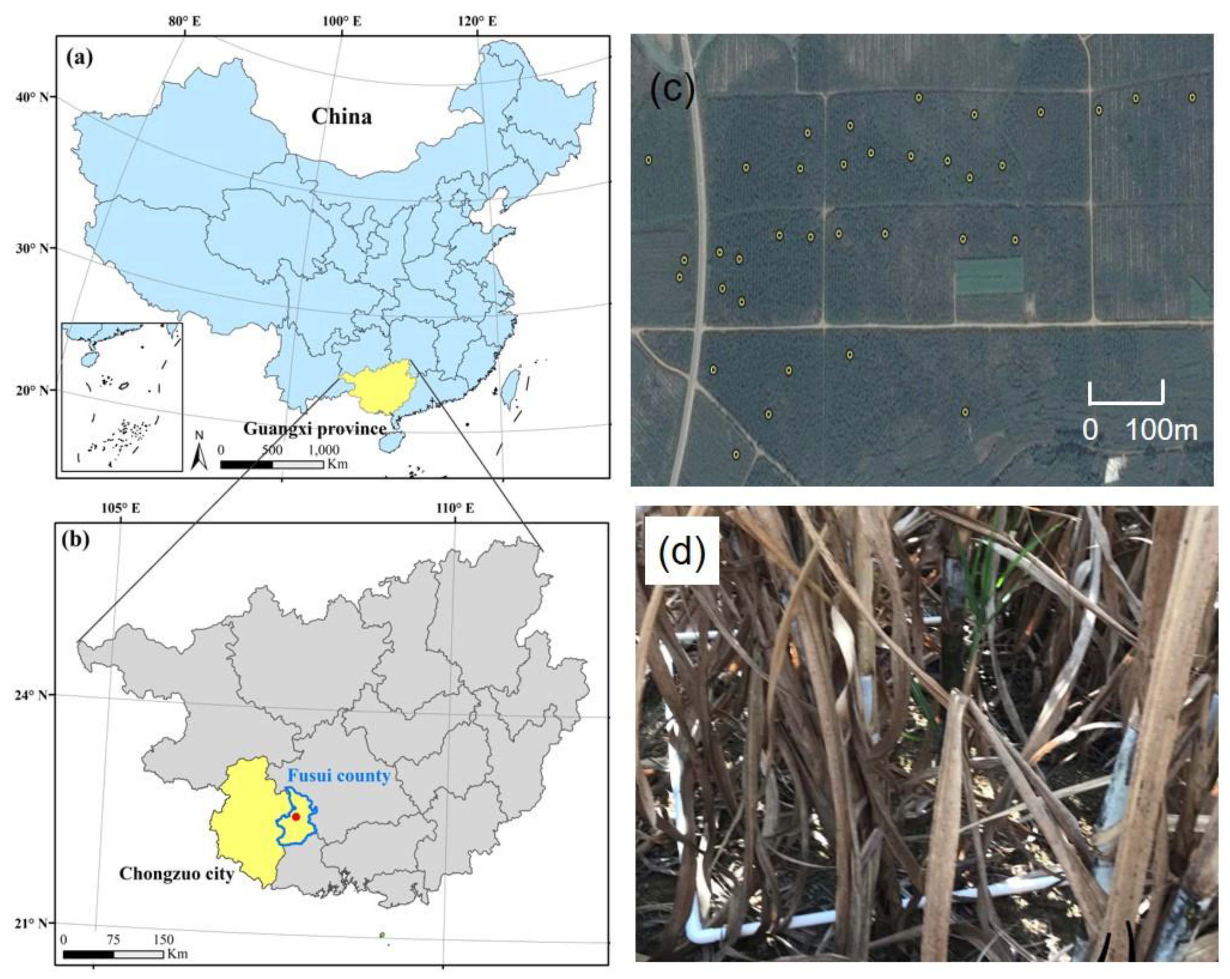
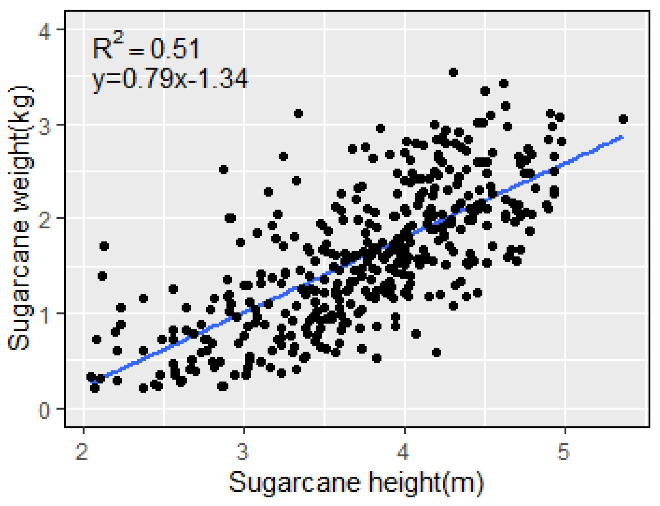
2.1. Study Area and Field Sampling

The study area is located in Fusui county (Figure 1), Chongzuo city of Guangxi province, and it extends across 22.55°N–22.57°N, 107.80°E–107.82°E. According to the Chongzuo Meteorological Bureau (http://www.chongzuo.gov.cn/zjcz/zrdl/t61340.shtml), the local mean annual temperature is 21.7 °C and the annual precipitation is approximately 1200 mm. Given its location in the subtropical monsoon climate zone, the climate characteristics are suitable for sugarcane cultivation.
Sugarcane is generally planted using two tillage methods (intensification and individualization) in early February and harvested in early December each year. The field sampling was accomplished in late November before ripening. We conducted a survey of thirty-five sites and each site contained three plots. In total, 105 sample plots 1 m × 1 m in size were randomly selected to obtain sugarcane inventory data. The geographic coordinates (longitude and latitude) of each plot were recorded using a GPSMAP 639csx from a Taiwan manufacturer, the GARMIN company. In each plot, we cut the aboveground part of all sugarcane plants and kept the leaves on the stem. The number of sugarcane plants in each plot ranged from nine to eighteen. The height and the fresh weight of each plant were measured.

2.2. UAV-LiDAR Data Preprocessing and LiDAR-Derived Metrics Extraction

We took four days in November 2019 to collect the raw UAV-LiDAR data based on an LR1601-IRIS Lidar point cloud data acquisition system that was installed on a DJI M600 UAV platform. The whole study area is about 1 km2 and the costs were roughly 2000 USD (United States dollar) in total. The main technical indicators of LiDAR are described in Table 1. In total, 52 remote sensing flying transects were collected to cover the entire area, and the overlap between adjacent routes was set to be greater than 30%. The flight altitude was 100 m above the ground with a uniform velocity of 1 m s−1. The WGS-84 coordinate system and UTM projection were used for the point cloud data.
The segmentation boundary of LiDAR data was established in Google Earth software and saved in KML format. Then we imported the path data together with LiDAR data into Point Cloud Producer software to obtain all the UAV-LiDAR point clouds. The point clouds dataset included five columns of information: easting, northing, elevation, intensity, and airline_ID. Point density was approximately 175 points m−2, which was dense enough to allow points to penetrate the sugarcane canopy and reach the exposed surface. The DEM (Digital Elevation Model) and DSM (Digital Surface Model) were generated using ENVI LiDAR software with a spatial resolution of 0.2 m. The height of sugarcane was obtained by subtracting DSM raster data and DEM raster data using ENVI 5.3.1 software. Then the average height, the variance of height, the square of average height, and the range of height with a spatial resolution of 1 m were calculated in ArcGIS 10.4 software. Lidar-derived variables have a high consistency with data from a field survey.

2.3. Different Regression Algorithms for Sugarcane AFW Prediction

Six different algorithms, including multiple linear regression (MLR), stepwise multiple regression (SMR), generalized linear model (GLM), generalized boosted model (GBM), kernel-based regularized least squares (KRLS), and random forest regression (RFR), were selected to construct the prediction models in our study. These models are classified into linear models and nonlinear models. R square (R2) and root mean square error (RMSE) between fitted and observed data were used as the evaluation index for model accuracy. The training set and test set contained 78 samples and 27 samples respectively.
Indicators related to height are commonly used to build models to estimate vegetation AGB [32,33]. Due to the significant positive correlation between sugarcane height and weight (Figure 2) which were measured in the field on individual plants, we selected eight field survey metrics as the appropriate variables. Details of the variables are summarized in Table 2. All regression algorithms were performed in R software (R version 3.6.1).

2.3.1. Linear Regression Model

MLR is a mathematical algorithm that uses multiple independent variables to obtain the predicted value. MLR models have been widely used in various scientific fields given their universality and well-founded theoretical basis [34]. To prevent collinearity, all-subsets regression was implemented using the “leaps” package in R to filter variables in the table. The general form of the formula is shown below:
y = β0 + β1 × 1 + β2 × 23 × 3 + …+ βnXn
where y is AFW in our study, β0 to βn are unknown linear regression coefficients, and X1 to Xn represent predictor variables.
SMR is a variable selection method of the MLR model that is used to gain the highest determination coefficient. The stepwise regression method combines forward selection with backward elimination, which is achieved by adding and deleting control variables according to the needs of each step [35]. Previous research has shown that the stepwise Akaike information criterion (AIC) method for variable selection is more appropriate than other stepwise methods [36]. As a result, we selected important variables from available variables based on the AIC principle. This study was conducted using the “stepwise” package in R statistical environment.

2.3.2. Machine Learning Regression Models

In machine learning regression algorithms, we chose GLM, GBM, KRLS, and RFR as predictive models. The response variable is the fresh weight of sugarcane, and the predictor variables are all shown in Table 2.
GLM is an extended form of the conventional linear model. Varied distributions (e.g., the normal, binomial, poisson, and gamma) are included in the GLM framework logistic. We chose “Poisson” regression because of its superiority in fitting the logarithmic model of variables.
We used a boosted regression tree (BRT) analysis in GBM and implemented the GBM model through the “gbm” package in R statistical environment. BRT combines the strengths of regression trees and boosting [37]. These strengths bring advantages in modeling non-parametric relationships between AFW and predictor variables.
KRLS applies the kernel trick to conduct regression estimation. It is a kind of machine learning approach that allows users to solve regression problems with the characteristics of ease-of-use and interpretability [38]. In particular, KRLS owns a flexible hypothesis space and provides closed-form estimates for the predicted values, which broaden the application range of the model. We implemented the KRLS model through the “KRLS” package in R statistical environment.
RFR is a well-known and powerful machine learning method proposed by Breiman [39] in which numerous decision trees are used to train and predict the sample. A large set of decision trees improves the classification and regression trees method [40]. In the process of model building, two main parameters must be optimized in this model: the number of decision trees (ntree) and the predictor used in the binary tree at each node selected at random (mtry). Finally, new data are obtained by averaging the predictions of all regression trees [41]. RFR has been widely used in the estimation of AGB given its outstanding characteristics such as insensitivity to noise in training data and nonlinear problems [39,42]. We implemented the RFR model through the “randomForest” package in R statistical environment.

2.4. Canopy Cover, the Distance to the Road and Tillage Method Information Extraction

To analyze agricultural management factors associated with sugarcane AFW, we considered canopy cover, the distance to the road, and tillage methods. Information extraction about corresponding yield with different managements was based on point clouds dataset (*.txt) and AFW raster data (*.dat), which were extracted from further LiDAR data analysis and programming in R software. Canopy cover is defined as the ratio of the vertical projection area of vegetation canopy to the total statistical area. Prior to calculating the canopy cover, the normalized point cloud data was generated in the LiDAR360 software. Then the normalized data were used as input data to generate the final results in the “canopy cover” function. We built six categories of the region of interest (ROI) in ENVI software according to the distances of the sugarcane planting area to the road: 0–2, 2–4, 4–6, 6–8, and 8–10 m and greater than 10 m. Tillage methods were divided into intensification and individualization according to the boundary of the farm. Intensive cultivation is within the business scope of local farms, and other farmland focuses on individual cultivation. Finally, we combined the canopy cover, the distance to the road, and tillage methods information with the predicted sugarcane yield information according to the longitude and latitude of each grid in ENVI Classic software. A significance test was conducted in R software.

3. Results

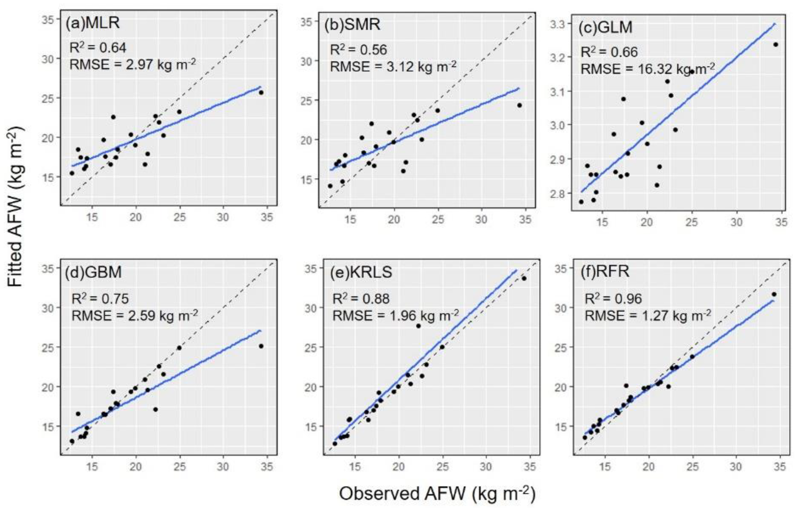
3.1. Performance of Different Algorithms for AFW Predictions

Figure 3 showed the fitting results of different models. Non-linear models exhibited significantly improved performance compared with the two linear models. Regarding machine learning methods, GLM, GBM, KRLS, and RFR, R2 gradually increased and RMSE gradually decreased. The RFR algorithm had the highest R2 and the lowest RMSE in all models.

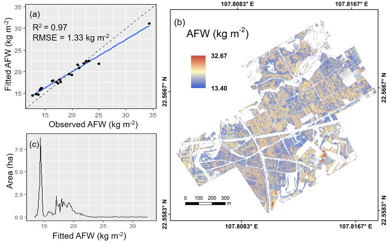
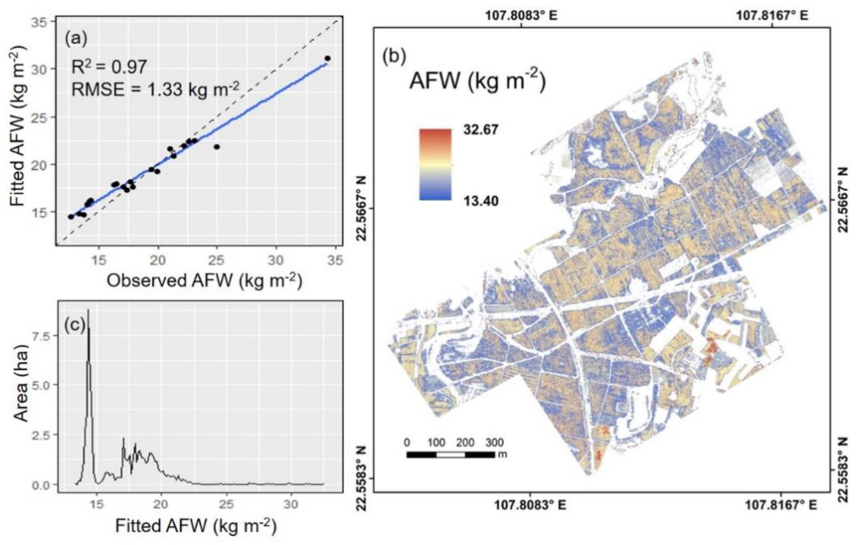
3.2. AFW Estimation Based on the RFR Model and LiDAR-Derived Data

Figure 4a depicted the scatter of the observed and fitted AFW based on the RFR model and LiDAR-derived data to detect the accuracy of the map. RMSE was 1.33 kg m−2, and the average AFW of sampling regions was 19.50 kg m−2, implying that the RMSE% was approximately 6.8%. Moreover, the fitting effect of the trend line had practical significance with an R2 as high as 0.97. The result confirmed the feasibility of using LiDAR point cloud data and RFR algorithms to estimate AFW of sugarcane. As noted in the AFW spatial distribution map (Figure 4b), AFW ranged from 13.40 kg m−2 to 32.67 kg m−2, different colors represented different AFW values. Figure 4c depicted the frequency distribution curve of predicted AFW, it reflected the planting area of sugarcane corresponding to different AFW. The majority of values were concentrated in the range of 14–22 kg m−2.

3.3. Analysis of Different Influencing Factors

The average values of AFW increased as the canopy cover increased. However, when canopy cover was greater than 0.7, the results were basically unchanged (Figure 5a). Moreover, AFW corresponding to a distance of 0–2 m to the road was evidently lower than others. In addition, slight changes were noted when the distance was greater than 2 m (Figure 5b). Regarding tillage methods, Figure 5c showed the differences between individualization and intensification. The average AFW values of sugarcane fields planted individually and intensively were approximately 16.84 kg m−2 and 17.43 kg m−2, respectively. Significant differences were noted between these two groups.

4. Discussion

4.1. Comparison of Diverse Regression Models

We explored the potential of building various regression models based on ground-measured data, including linear and nonlinear algorithms. Except for GLM, nonlinear models outperformed linear models in the accuracy of predictions. The considerations regarding the respective characteristics of different mathematical models and the selection and assessment of predictive variables were determined according to different standards, and the variable importance of regression was an important principle [43]. All-subsets regression was applied to avoid multicollinearity in the traditional linearity model. The average height of sugarcane was ignored in SMR based on the lowest AIC value.
RFR is a highly recommended machine learning approach to establish a complex nonlinear relationship, that tends to confer importance between multiple predictors [44]. A possible explanation for the increased superior performance of RFR is that each tree is independent, and each variable can demonstrate significance in different trees. Furthermore, the RFR model has solved the problem of collinearity and overfitting during AFW estimation. Previous studies have successfully demonstrated that the RFR model is applicable to make an accurate prediction of sugarcane yield [45,46] and our conclusion is consistent with them. When comparing the accuracy of all models, the highest R2 (0.96) and the lowest RMSE (1.27 kg m−2) indicated that RFR was the most appropriate model for the estimation of sugarcane AFW. Scornet et al. [47] suggested that the ability to deal with small sample sizes was conducive to the popularity of RFR methodology. In our study, we accomplished surveys of thirty-five field sites, which contained 105 plots. Increasing field measurements for further analysis on the influence of sample numbers on the prediction results of the model is the focus of our future research.

4.2. The Feasibility of UAV-LiDAR Data for AFW Prediction

As an active remote sensing technology with rapid development, UAV-LiDAR has distinct advantages compared with traditional LiDAR platforms (satellite, aerial, and terrestrial), such as easy operability, lightweight, financial viability, and flexibility in acquisition and sensor integration [48,49]. Most importantly, UAV laser scanning systems provide higher point density accompanying with lower speeds and altitudes than airborne laser scanning [50]. Detailed characteristics can be extracted from the denser point cloud [51,52]. Yin and Wang [53] realized individual tree detection and delineation using LiDAR data (91 points m−2) collected from UAV, including height, crown diameter, and crown clumping density. Almeida et al. [54] monitored the structure of mixed-species forest restoration plantations with three structural variables (canopy height, gap fraction, and leaf area index) from the UAV-borne LiDAR system, and obtained a high R2 (0.84) for AGB. Most of the previous studies focused on the application of UAV-LiDAR data in the prediction of forest AGB, whereas our study demonstrated that it is also feasible to use this technology for sugarcane.
In our study, data captured from UAV-LiDAR was well suited for AFW prediction and generation of sugarcane AFW maps in the specific study region. We analyzed several features related to vegetation height from LiDAR data with an average density of 175 points m−2, which significantly contributes to the precise sugarcane AFW estimation (R2 = 0.97 and RMSE = 1.33 kg m−2) with fine spatial resolution. The multirotor UAV provided a stable platform for the LiDAR sensor by reducing vibration. On the one hand, the morphological structure of sugarcane is simple, making it convenient for LiDAR to detect vegetation structure information. On the other hand, the sugarcane plant is much higher than other crops, such as rice, wheat and so on, which is conducive to the recognition of sugarcane in point cloud data if they are planted adjacent to other crops. In addition, the positive correlation between sugarcane height and weight also contributes to the accuracy of the results.
Given the abovementioned advantages and availability of lighter LiDAR sensors in the future, the UAV-borne lidar system will cover a wider range of application functions. This study may pave the way for further analysis of UAV-LiDAR systems and large-scale sugarcane AFW estimations. The fusion of multisource remote sensing may bring vitality to future research. New generation technologies, such as NASA’s Global Ecosystem Dynamics Investigation (GEDI), NASA’s Ice Cloud and land Elevation Satellite (ICESat−2), and the NASA-Indian Space Research Organization (ISRO) Synthetic Aperture Radar (NISAR), have the potential to collect useful data for estimating biomass at a national or global scale [55].

4.3. Insight on Agricultural Management on Sugarcane Production

We investigated the influence of agricultural management factors, including canopy cover, the distance to the road, and tillage methods, on sugarcane AFW in our study. Our results have profound significance for combining scientific research with practical application for the purpose of enhancing sugarcane yield.
Sugarcane is planted in the form of seedlings. Canopy cover directly responds to planting density. The emergence of competition mechanisms explains why the increase in the sugarcane population is not equal to a bumper harvest. Competitive interaction among individuals affected the effective use of resources, mainly including solar energy, soil nutrients, and soil moisture. Different crops have different optimum planting density. Moderate to high density is a scientific approach for improving lint yield under a late sowing date [56]. Low-density triticale regardless of cultivar performed best in low rainfall regions across the Mediterranean Basin [57]. Our results clearly demonstrate that a canopy cover of 0.6–0.7 can make the most effective use of germplasm resources. In addition to the interference of individual competition, the distance to the road also has a significant impact on AFW. Figure 5b demonstrates poor sugarcane growth in the area closest to the road, and the influence of human activities (e.g., the trampling of people and the rolling of vehicles) may represent the best explanation for this observation. In addition to the negative effects of human activities, moisture is likely to evaporate and nutrient is likely to be lost in marginal soil because the release of organic carbon and nitrogen from litter are inhibited in the marginal area [58], which can also lead to a reduction in sugarcane production. Sustainable agricultural intensification is a primary trend of land use to feed a growing population [59,60]. It can achieve many functions, including but not limited to greenhouse gas mitigation [61] and high energy efficiency [62]. The results (Figure 4c) demonstrate that intensive cultivation is worth popularizing because it can effectively improve AFW. Sustainable intensification was practiced from 1980 to 2014 in Northern China with sustained high crop production [63]. China’s agriculture is still in the transition stage from conventional agriculture to modern agriculture. Increased crop production can be realized by further agricultural intensification rather than expanding the cultivated land area [64]. In the long term, popularizing farming systems for sustainable intensification must continue to be pursued in the future.

5. Conclusions

In our study, the effectiveness of UAV-LiDAR data is demonstrated by providing proper metrics according to the sugarcane structural parameters. We evaluated the capacity of different regression algorithms (i.e., MLR, SMR, GLM, GBM, KRLS, and RFR) to estimate sugarcane AFW. The RFR model outperforms other regression models in terms of the accuracy of prediction, providing an important method for mapping the spatial distribution of sugarcane AFW with high resolution. Furthermore, the derived sugarcane AFW map demonstrates the capacity for further analysis of the influence of agricultural management factors, including the planting density, the distance to the road, and tillage methods. The main contribution of our research results is the ability to supply theoretical support for practical farming. We believe that increased sugarcane yield is possible via the scientific calculation of the optimum planting density, the reduction of negative effects caused by human activities, and the choice of suitable tillage methods.

Author Contributions

Conceptualization, J.-X.X. and J.M.; Data curation, W.-X.W. and J.-H.S.; Investigation, J.-X.X., Y.-N.T., W.-B.W., S.-Y.W., Y.-F.L., Y.-C.W. and H.-Q.G.; Methodology, J.-X.X., J.M. and Y.-N.T.; Writing—original draft, J.-X.X.; Writing—review & editing, J.M. All authors have read and agreed to the published version of the manuscript.

Funding

This research was supported by the National Key Research and Development Program of China (2017YFC1200100), the Natural Science Foundation of China (41601181), Guangxi key research and development program (Gui Ke AB19245040), the Open Research Fund of the Guangxi Key Laboratory of Water Engineering Materials and Structures, Guangxi Hydraulic Research Institute (GXHRI-WEMS-2020-07), and the Scientific Research Program of Shanghai Science and Technology Commission (20dz1204702).

Acknowledgments

We thank Zhenping Huang from Guangxi Institute of Water Resources Research for the help in field investigation. We also gratefully acknowledge all the reviewers for their time and effort in reviewing our manuscripts and providing valuable suggestions and comments.

Conflicts of Interest

The authors declare no conflict of interest.

References

  1. Rocha, F.R.; Papini-Terzi, F.S.; Nishiyama, M.Y., Jr.; Vencio, R.Z.; Vicentini, R.; Duarte, R.D.; de Rosa, V.E., Jr.; Vinagre, F.; Barsalobres, C.; Medeiros, A.H.; et al. Signal transduction-related responses to phytohormones and environmental challenges in sugarcane. BMC Genom. 2007, 8, 71. [Google Scholar] [CrossRef] [Green Version]
  2. Suprasanna, P.; Patade, V.Y.; Desai, N.S.; Devarumath, R.M.; Kawar, P.G.; Pagariya, M.C.; Ganapathi, A.; Manickavasagam, M.; Babu, K.H. Biotechnological developments in sugarcane improvement: An overview. Sugar Tech. 2011, 13, 322–335. [Google Scholar] [CrossRef]
  3. Jayapal, N.; Samanta, A.K.; Kolte, A.P.; Senani, S.; Sridhar, M.; Suresh, K.P.; Sampath, K.T. Value addition to sugarcane bagasse: Xylan extraction and its process optimization for xylooligosaccharides production. Ind. Crops Prod. 2013, 42, 14–24. [Google Scholar] [CrossRef]
  4. Goncalves, T.A.; Damasio, A.R.; Segato, F.; Alvarez, T.M.; Bragatto, J.; Brenelli, L.B.; Citadini, A.P.; Murakami, M.T.; Ruller, R.; Paes Leme, A.F.; et al. Functional characterization and synergic action of fungal xylanase and arabinofuranosidase for production of xylooligosaccharides. Bioresour. Technol. 2012, 119, 293–299. [Google Scholar] [CrossRef] [Green Version]
  5. Pereira, S.C.; Maehara, L.; Machado, C.M.M.; Farinas, C.S. Physical–chemical–morphological characterization of the whole sugarcane lignocellulosic biomass used for 2G ethanol production by spectroscopy and microscopy techniques. Renew. Energy 2016, 87, 607–617. [Google Scholar] [CrossRef]
  6. David, T.; Robert, S.; Jonathan, A.F.; Jason, H.; Eric, L.; Lee, L.; Stephen, P.; John, R.; Tim, S.; Chris, S.; et al. Beneficial biofuels—The food, energy, and environment trilemma. Science 2009. [Google Scholar] [CrossRef] [Green Version]
  7. Li, Y.-R.; Yang, L.-T. Sugarcane agriculture and sugar industry in China. Sugar Tech. 2015, 17, 1–8. [Google Scholar] [CrossRef]
  8. Atzberger, C. Advances in remote sensing of agriculture: Context description, existing operational monitoring systems and major information needs. Remote Sens. 2013, 5, 949–981. [Google Scholar] [CrossRef] [Green Version]
  9. Chao, Z.; Liu, N.; Zhang, P.; Ying, T.; Song, K. Estimation methods developing with remote sensing information for energy crop biomass: A comparative review. Biomass Bioenergy 2019, 122, 414–425. [Google Scholar] [CrossRef]
  10. Rembold, F.; Atzberger, C.; Savin, I.; Rojas, O. Using Low Resolution Satellite Imagery for Yield Prediction and Yield Anomaly Detection. Remote Sens. 2013, 5, 1704–1733. [Google Scholar] [CrossRef] [Green Version]
  11. Hoffmeister, D.; Waldhoff, G.; Korres, W.; Curdt, C.; Bareth, G. Crop height variability detection in a single field by multi-temporal terrestrial laser scanning. Precis. Agric. 2016, 17, 296–312. [Google Scholar] [CrossRef]
  12. Dubayah, R.O.; Drake, J.B. Lidar remote sensing for forestry. J. For. 2000, 98, 44–46. [Google Scholar]
  13. Koch, B. Status and future of laser scanning, synthetic aperture radar and hyperspectral remote sensing data for forest biomass assessment. ISPRS J. Photogramm. Remote Sens. 2010, 65, 581–590. [Google Scholar] [CrossRef]
  14. Lefsky, M.A.; Cohen, W.B.; Harding, D.J.; Parker, G.G.; Acker, S.A.; Gower, S.T. Lidar Remote sensing of above-ground biomass in three biomes. Glob. Ecol. Biogeogr. 2002, 11, 393–399. [Google Scholar] [CrossRef] [Green Version]
  15. Wu, Z.; Dye, D.; Vogel, J.; Middleton, B. Estimating forest and woodland aboveground biomass using active and passive remote sensing. Photogramm. Eng. Remote Sens. 2016, 82, 271–281. [Google Scholar] [CrossRef]
  16. Knapp, N.; Fischer, R.; Huth, A. Linking lidar and forest modeling to assess biomass estimation across scales and disturbance states. Remote Sens. Environ. 2018, 205, 199–209. [Google Scholar] [CrossRef]
  17. Wulder, M.A.; White, J.C.; Nelson, R.F.; Næsset, E.; Ørka, H.O.; Coops, N.C.; Hilker, T.; Bater, C.W.; Gobakken, T. Lidar sampling for large-area forest characterization: A review. Remote Sens. Environ. 2012, 121, 196–209. [Google Scholar] [CrossRef] [Green Version]
  18. Kaasalainen, S.; Holopainen, M.; Karjalainen, M.; Vastaranta, M.; Kankare, V.; Karila, K.; Osmanoglu, B. Combining lidar and synthetic aperture radar data to estimate forest biomass: Status and prospects. Forests 2015, 6, 252–270. [Google Scholar] [CrossRef]
  19. Vaglio Laurin, G.; Puletti, N.; Chen, Q.; Corona, P.; Papale, D.; Valentini, R. Above ground biomass and tree species richness estimation with airborne lidar in tropical Ghana forests. Int. J. Appl. Earth Obs. Geoinf. 2016, 52, 371–379. [Google Scholar] [CrossRef] [Green Version]
  20. Bouvier, M.; Durrieu, S.; Fournier, R.A.; Renaud, J.P. Generalizing predictive models of forest inventory attributes using an area-based approach with airborne LiDAR data. Remote Sens. Environ. 2015, 156, 322–334. [Google Scholar] [CrossRef]
  21. Li, W.; Niu, Z.; Huang, N.; Wang, C.; Gao, S.; Wu, C. Airborne LiDAR technique for estimating biomass components of maize: A case study in Zhangye City, Northwest China. Ecol. Indic. 2015, 57, 486–496. [Google Scholar] [CrossRef]
  22. Wallace, L.; Lucieer, A.; Watson, C.; Turner, D. Development of a UAV-LiDAR system with application to forest inventory. Remote Sens. 2012, 4, 1519–1543. [Google Scholar] [CrossRef] [Green Version]
  23. Jeong, J.H.; Resop, J.P.; Mueller, N.D.; Fleisher, D.H.; Yun, K.; Butler, E.E.; Timlin, D.J.; Shim, K.M.; Gerber, J.S.; Reddy, V.R.; et al. Random forests for global and regional crop yield predictions. PLoS ONE 2016, 11, e0156571. [Google Scholar] [CrossRef] [PubMed]
  24. Han, L.; Yang, G.; Dai, H.; Xu, B.; Yang, H.; Feng, H.; Li, Z.; Yang, X. Modeling maize above-ground biomass based on machine learning approaches using UAV remote-sensing data. Plant. Methods 2019, 15, 10. [Google Scholar] [CrossRef] [PubMed] [Green Version]
  25. Feng, P.; Wang, B.; Liu, D.L.; Waters, C.; Xiao, D.; Shi, L.; Yu, Q. Dynamic wheat yield forecasts are improved by a hybrid approach using a biophysical model and machine learning technique. Agric. For. Meteorol. 2020, 285–286. [Google Scholar] [CrossRef]
  26. González-Sanchez, A.; Frausto-Solis, J.; Ojeda, W. Predictive ability of machine learning methods for massive crop yield prediction. Span. J. Agric. Res. 2014. [Google Scholar] [CrossRef] [Green Version]
  27. Van Klompenburg, T.; Kassahun, A.; Catal, C. Crop yield prediction using machine learning: A systematic literature review. Comput. Electron. Agric. 2020, 177, 105709. [Google Scholar] [CrossRef]
  28. Chlingaryan, A.; Sukkarieh, S.; Whelan, B. Machine learning approaches for crop yield prediction and nitrogen status estimation in precision agriculture: A review. Comput. Electron. Agric. 2018, 151, 61–69. [Google Scholar] [CrossRef]
  29. Leroux, L.; Castets, M.; Baron, C.; Escorihuela, M.-J.; Bégué, A.; Lo Seen, D. Maize yield estimation in West Africa from crop process-induced combinations of multi-domain remote sensing indices. Eur. J. Agron. 2019, 108, 11–26. [Google Scholar] [CrossRef]
  30. Sakamoto, T. Incorporating environmental variables into a MODIS-based crop yield estimation method for United States corn and soybeans through the use of a random forest regression algorithm. ISPRS J. Photogramm. Remote Sens. 2020, 160, 208–228. [Google Scholar] [CrossRef]
  31. Gyamerah, S.A.; Ngare, P.; Ikpe, D. Probabilistic forecasting of crop yields via quantile random forest and Epanechnikov Kernel function. Agric. For. Meteorol. 2020, 280, 107808. [Google Scholar] [CrossRef]
  32. Tsui, O.W.; Coops, N.C.; Wulder, M.A.; Marshall, P.L.; McCardle, A. Using multi-frequency radar and discrete-return LiDAR measurements to estimate above-ground biomass and biomass components in a coastal temperate forest. ISPRS J. Photogramm. Remote Sens. 2012, 69, 121–133. [Google Scholar] [CrossRef]
  33. Kankare, V.; Räty, M.; Yu, X.; Holopainen, M.; Vastaranta, M.; Kantola, T.; Hyyppä, J.; Hyyppä, H.; Alho, P.; Viitala, R. Single tree biomass modelling using airborne laser scanning. ISPRS J. Photogramm. Remote Sens. 2013, 85, 66–73. [Google Scholar] [CrossRef]
  34. Araiza, J.; Rojas-Valencia, M.; Vera, R. Forecast generation model of municipal solid waste using multiple linear regression. Glob. J. Environ. Sci. Manag. 2019, 6, 1–14. [Google Scholar] [CrossRef]
  35. Ghani, I.M.M.; Ahmad, S. Stepwise multiple regression method to forecast fish landing. Procedia Soc. Behav. Sci. 2010, 8, 549–554. [Google Scholar] [CrossRef] [Green Version]
  36. Yamashita, T.; Yamashita, K.; Kamimura, R. A Stepwise AIC Method for variable selection in linear regression. Commun. Stat. Theory Methods 2007, 36, 2395–2403. [Google Scholar] [CrossRef]
  37. Elith, J.; Leathwick, J.R.; Hastie, T. A working guide to boosted regression trees. J. Anim. Ecol. 2008, 77, 802–813. [Google Scholar] [CrossRef]
  38. Hainmueller, J.; Hazlett, C. Kernel regularized least squares: Reducing misspecification bias with a flexible and interpretable machine learning approach. Political Anal. 2014, 22, 143–168. [Google Scholar] [CrossRef]
  39. Breiman, L. Random forests. Mach. Learn. 2001, 45, 5–32. [Google Scholar] [CrossRef] [Green Version]
  40. Ramoelo, A.; Cho, M.A.; Mathieu, R.; Madonsela, S.; van de Kerchove, R.; Kaszta, Z.; Wolff, E. Monitoring grass nutrients and biomass as indicators of rangeland quality and quantity using random forest modelling and WorldView-2 data. Int. J. Appl. Earth Obs. Geoinf. 2015, 43, 43–54. [Google Scholar] [CrossRef]
  41. Pham, L.T.H.; Brabyn, L. Monitoring mangrove biomass change in Vietnam using SPOT images and an object-based approach combined with machine learning algorithms. ISPRS J. Photogramm. Remote Sens. 2017, 128, 86–97. [Google Scholar] [CrossRef]
  42. Heung, B.; Bulmer, C.E.; Schmidt, M.G. Predictive soil parent material mapping at a regional-scale: A Random Forest approach. Geoderma 2014, 214–215, 141–154. [Google Scholar] [CrossRef]
  43. Grömping, U. Variable importance assessment in regression: Linear regression versus random forest. Am. Stat. 2009, 63, 308–319. [Google Scholar] [CrossRef]
  44. Freeman, E.A.; Moisen, G.G.; Coulston, J.W.; Wilson, B.T. Random forests and stochastic gradient boosting for predicting tree canopy cover: Comparing tuning processes and model performance. Can. J. For. Res. 2016, 46, 323–339. [Google Scholar] [CrossRef] [Green Version]
  45. Everingham, Y.; Sexton, J.; Skocaj, D.; Inman-Bamber, G. Accurate prediction of sugarcane yield using a random forest algorithm. Agric. Sustain. Develop. 2016, 36, 27. [Google Scholar] [CrossRef] [Green Version]
  46. Charoen-Ung, P.; Mittrapiyanuruk, P. Sugarcane Yield Grade Prediction using random forest with forward feature selection and hyper-parameter tuning. In Recent Advances in Information and Communication Technology; Springer: New York, NY, USA, 2019; pp. 33–42. [Google Scholar] [CrossRef]
  47. Scornet, E.; Biau, G.; Vert, J.-P. Consistency of random forests. Ann. Stat. 2015, 43, 1716–1741. [Google Scholar] [CrossRef]
  48. Pilarska, M.; Ostrowski, W.; Bakuła, K.; Górski, K.; Kurczyński, Z. The potential of light laser scanners developed for unmanned aerial vehicles—The review and accuracy. Int. Arch. Photogramm. Remote Sens. Spat. Inf. Sci. 2016, 42, 87–95. [Google Scholar] [CrossRef] [Green Version]
  49. Yao, H.; Qin, R.; Chen, X. Unmanned aerial vehicle for remote sensing applications—A review. Remote Sens. 2019, 11, 1443. [Google Scholar] [CrossRef] [Green Version]
  50. Beland, M.; Parker, G.; Sparrow, B.; Harding, D.; Chasmer, L.; Phinn, S.; Antonarakis, A.; Strahler, A. On promoting the use of lidar systems in forest ecosystem research. For. Ecol. Manag. 2019, 450. [Google Scholar] [CrossRef]
  51. Tesfamichael, S.G.; van Aardt, J.; Roberts, W.; Ahmed, F. Retrieval of narrow-range LAI of at multiple lidar point densities: Application on Eucalyptus grandis plantation. Int. J. Appl. Earth Obs. Geoinf. 2018, 70, 93–104. [Google Scholar] [CrossRef]
  52. Jaakkola, A.; Hyypp, J.; Kukko, A.; Yu, X.; Kaartinen, H.; LehtomäKi, M.; Yi, L. A low-cost multi-sensoral mobile mapping system and its feasibility for tree measurements. ISPRS J. Photogramm. Remote Sens. 2010, 65, 514–522. [Google Scholar] [CrossRef]
  53. Yin, D.; Wang, L. Individual mangrove tree measurement using UAV-based LiDAR data: Possibilities and challenges. Remote Sens. Environ. 2019, 223, 34–49. [Google Scholar] [CrossRef]
  54. Almeida, D.R.A.; Broadbent, E.N.; Zambrano, A.M.A.; Wilkinson, B.E.; Ferreira, M.E.; Chazdon, R.; Meli, P.; Gorgens, E.B.; Silva, C.A.; Stark, S.C.; et al. Monitoring the structure of forest restoration plantations with a drone-lidar system. Int. J. Appl. Earth Obs. Geoinf. 2019, 79, 192–198. [Google Scholar] [CrossRef]
  55. Duncanson, L.; Neuenschwander, A.; Hancock, S.; Thomas, N.; Fatoyinbo, T.; Simard, M.; Silva, C.A.; Armston, J.; Luthcke, S.B.; Hofton, M.; et al. Biomass estimation from simulated GEDI, ICESat-2 and NISAR across environmental gradients in Sonoma County, California. Remote Sens. Environ. 2020, 242. [Google Scholar] [CrossRef]
  56. Khan, A.; Najeeb, U.; Wang, L.; Tan, D.K.Y.; Yang, G.; Munsif, F.; Ali, S.; Hafeez, A. Planting density and sowing date strongly influence growth and lint yield of cotton crops. Field Crops Res. 2017, 209, 129–135. [Google Scholar] [CrossRef]
  57. Bassu, S.; Asseng, S.; Giunta, F.; Motzo, R. Optimizing triticale sowing densities across the Mediterranean Basin. Field Crops Res. 2013, 144, 167–178. [Google Scholar] [CrossRef]
  58. Miao, R.H.; Ma, J.; Liu, Y.Z.; Liu, Y.C.; Yang, Z.L.; Guo, M.X. Variability of aboveground litter inputs alters soil carbon and nitrogen in a coniferous–broadleaf mixed forest of Central China. Forests 2019, 10, 188. [Google Scholar] [CrossRef] [Green Version]
  59. Tilman, D.; Balzer, C.; Hill, J.; Befort, B.L. Global food demand and the sustainable intensification of agriculture. Proc. Natl. Acad. Sci. USA 2011, 108, 20260–20264. [Google Scholar] [CrossRef] [Green Version]
  60. Hunter, M.C.; Smith, R.G.; Schipanski, M.E.; Atwood, L.W.; Mortensen, D.A. Agriculture in 2050: Recalibrating targets for sustainable intensification. Bioscience 2017, 67, 386–391. [Google Scholar] [CrossRef] [Green Version]
  61. Burney, J.A.; Davis, S.J.; Lobell, D.B. Greenhouse gas mitigation by agricultural intensification. Proc. Natl. Acad. Sci. USA 2010, 107, 12052–12057. [Google Scholar] [CrossRef] [Green Version]
  62. Quilty, J.R.; McKinley, J.; Pede, V.O.; Buresh, R.J.; Correa, T.Q., Jr.; Sandro, J.M. Energy efficiency of rice production in farmers’ fields and intensively cropped research fields in the Philippines. Field Crops Res. 2014, 168, 8–18. [Google Scholar] [CrossRef]
  63. Zhang, X.; Bol, R.; Rahn, C.; Xiao, G.; Meng, F.; Wu, W. Agricultural sustainable intensification improved nitrogen use efficiency and maintained high crop yield during 1980–2014 in Northern China. Sci. Total Environ. 2017, 596–597, 61–68. [Google Scholar] [CrossRef] [PubMed]
  64. Meng, Q.; Hou, P.; Wu, L.; Chen, X.; Cui, Z.; Zhang, F. Understanding production potentials and yield gaps in intensive maize production in China. Field Crops Res. 2013, 143, 91–97. [Google Scholar] [CrossRef] [Green Version]
Figure 1. Study area and sampling plots. (a) The location of the Guangxi province in China; (b) Detailed map of the experimental site in Fusui county of Chongzuo city. The red dot is the field sampling area. (c) Spatial distribution of the field measurement sites. (d) An example of a 1 m × 1 m field plot. The white part is the sampling frame.
Remotesensing 12 02823 g001
Figure 2. Relationship between sugarcane weight and sugarcane height. The blue solid line represents a linear fit. Weight is positively correlated with height.
Remotesensing 12 02823 g002
Figure 3. Relationship between observed aboveground fresh weight (AFW) and fitted AFW of sugarcane via the six regression algorithms based on sampling plots. (a) multiple linear regression (MLR); (b) stepwise multiple regression (SMR); (c) generalized linear model (GLM); (d) generalized boosted model (GBM); (e) kernel-based regularized least squares (KRLS); (f) random forest regression (RFR). The black dotted line represents the 1:1 line, and the blue solid line represents a linear fit.
Remotesensing 12 02823 g003
Figure 4. (a) Relationship between observed aboveground fresh weight (AFW) and fitted AFW of sugarcane via random forest regression (RFR) algorithms based on LiDAR point cloud data. (b) The predicted sugarcane AFW map of the study area derived from RFR algorithms at 1 m spatial resolution. (c) Frequency distribution curve of predicted AFW.
Remotesensing 12 02823 g004
Figure 5. The influence of canopy cover, the distance to the road, and tillage method on the performance of sugarcane aboveground fresh weight (AFW). (a) Gray dots represent the average AFW value. (b) Orange dots represent the average value of AFW. (c) Blue dots represent the average AFW value. Stars indicate a significant difference between individualization and intensification (p < 0.001).
Remotesensing 12 02823 g005
Table 1. Main technical parameters of the LR1601-IRIS laser scanner system.
ParametersSpecification
Scanning frequency320,000 Hz
Number of sensors16
Maximum measurement distance150 m
Ranging accuracy±2 cm
Scan field angle360° × 30°
Location accuracy (horizontal/vertical)<0.01/<0.05 m (PPK RTK)
Pitch and roll (RMS)0.01°/0.05° (PPK RTK)
Velocity measurement precision0. 03 m s−1
Table 2. Statistical summary of the characteristics captured from 105 sampling plots.
ParameterMetricsDescription
X1H.meanAverage height (m) of sugarcane in a quadrat plot
X2H.maxMaximum height (m)
X3H.minMinimum height (m)
X4H.normalizedNormalization is between zero and one
X5H.sdStandard deviation of sugarcane height (m)
X6H.varVariance of sugarcane height (m2)
X7H.mean squaredH.mean ∗ H.mean
X8H.rangeH.max–H.min

