Perennial Supraglacial Lakes in Northeast Greenland Observed by Polarimetric SAR


Abstract

1. Introduction
2. Data and Methods
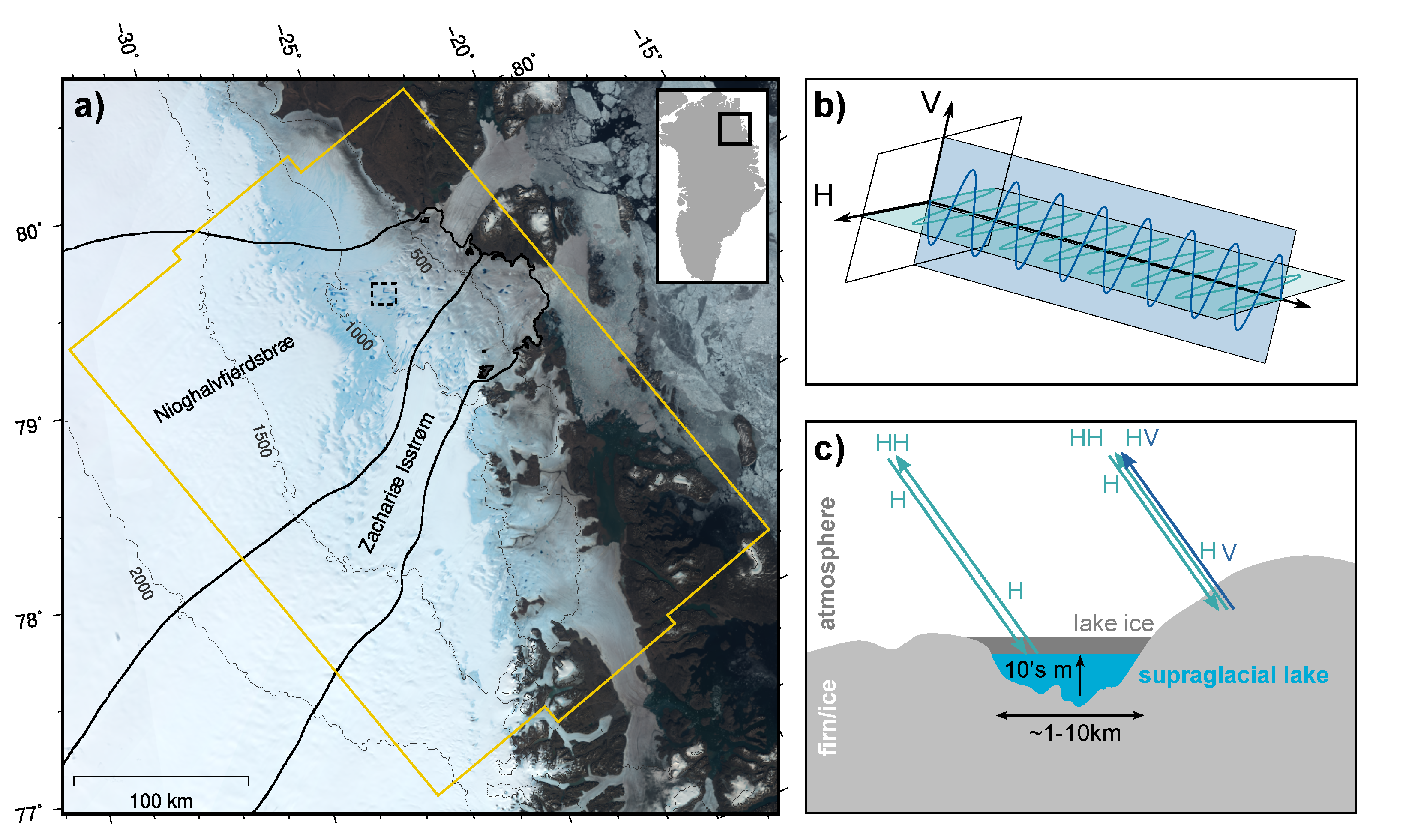
2.1. Sentinel-1 Backscatter
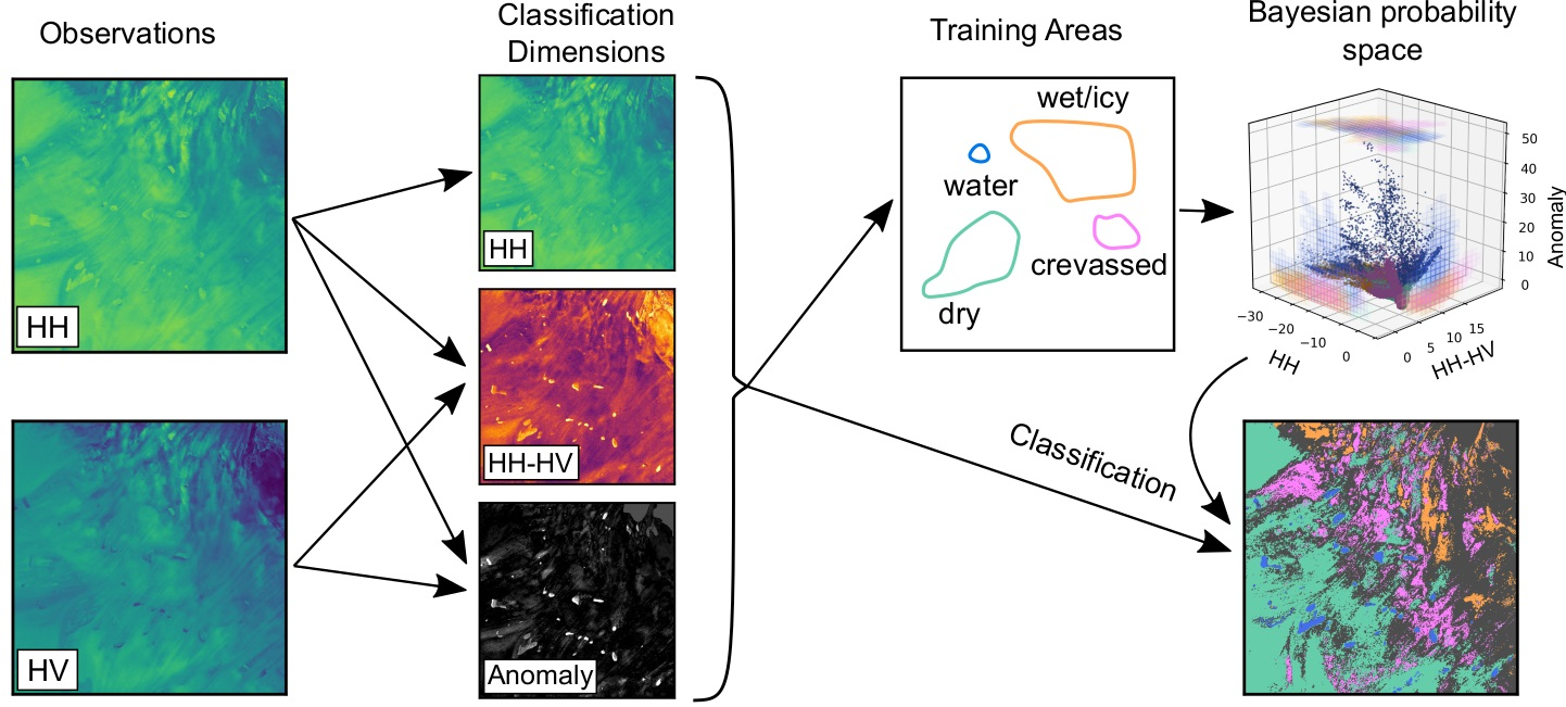
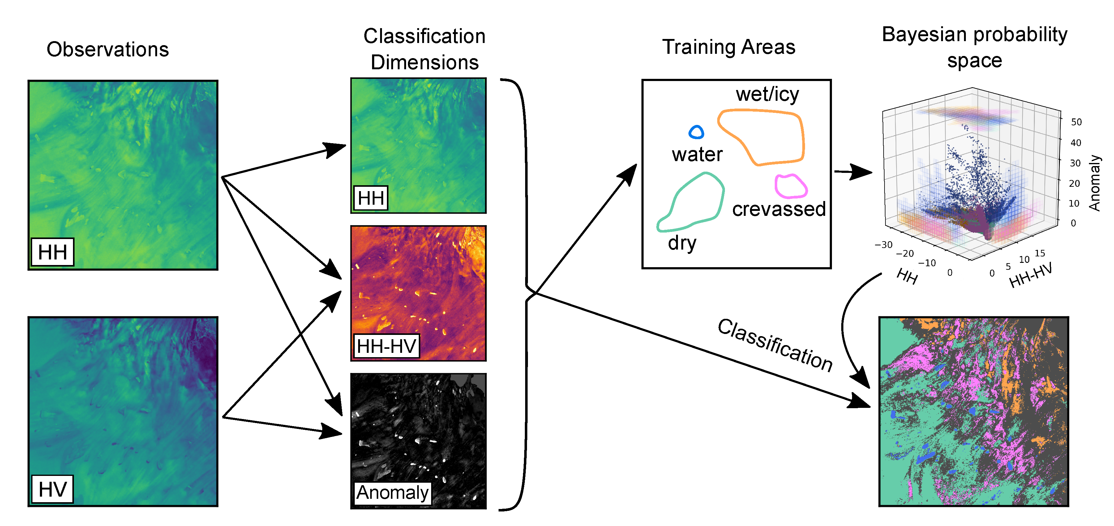
2.2. Classification
2.3. Supraglacial Lake Definition
2.4. Complementary Optical Data
3. Results
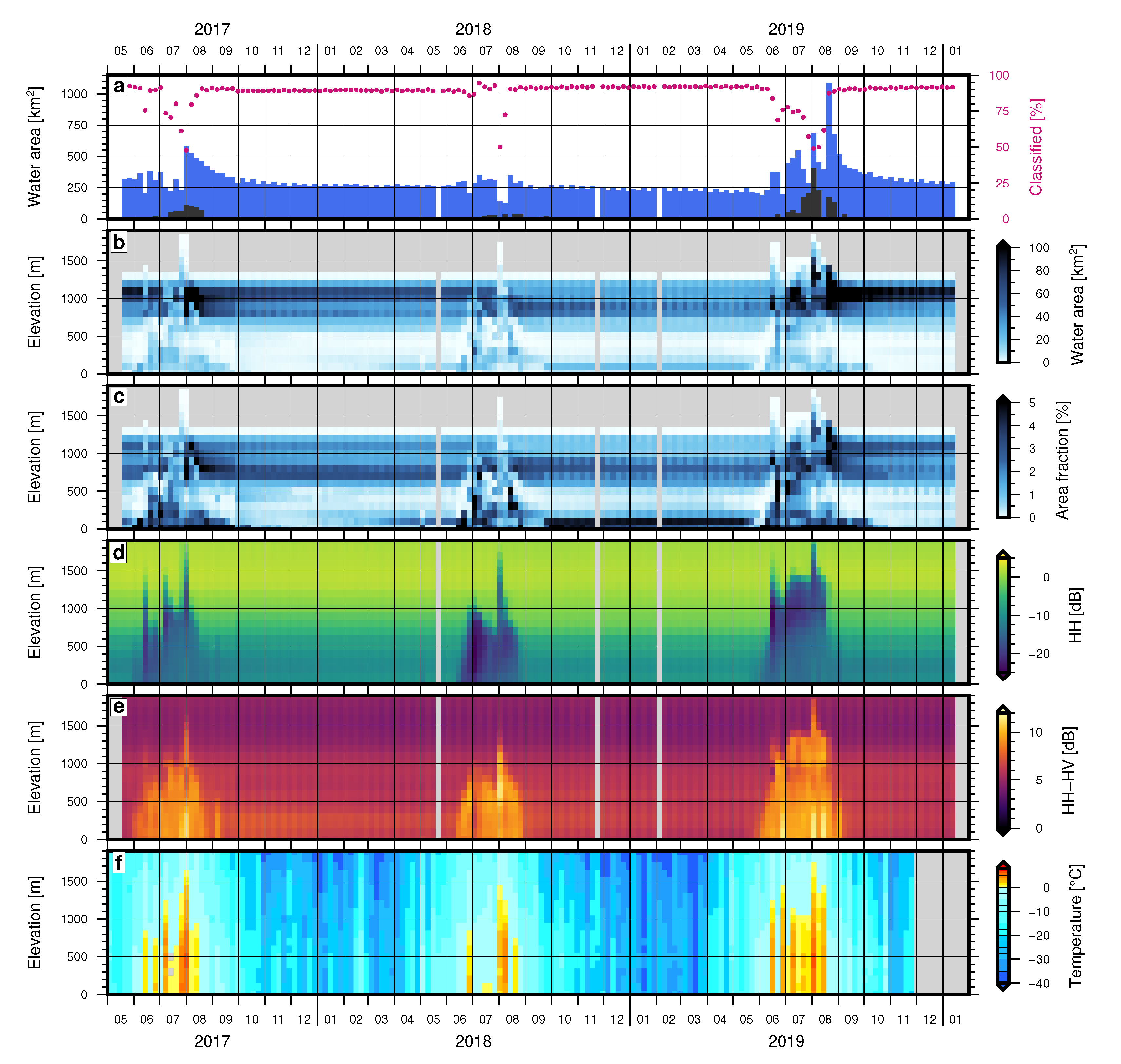
3.1. Time Series
3.2. Validation
3.3. Lake Drainage
4. Discussion
5. Conclusions
Supplementary Materials
Author Contributions
Funding
Acknowledgments
Conflicts of Interest
References
- Echelmeyer, K.; Clarke, T.S.; Harrison, W. Surficial glaciology of Jakobshavns Isbræ, West Greenland: Part I. Surface morphology. J. Glaciol. 1991, 37, 368–382. [Google Scholar] [CrossRef][Green Version]
- Lüthje, M.; Pedersen, L.; Reeh, N.; Greuell, W. Modelling the evolution of supraglacial lakes on the West Greenland ice-sheet margin. J. Glaciol. 2006, 52, 608–618. [Google Scholar] [CrossRef]
- Tedesco, M.; Lüthje, M.; Steffen, K.; Steiner, N.; Fettweis, X.; Willis, I.; Bayou, N.; Banwell, A. Measurement and modeling of ablation of the bottom of supraglacial lakes in western Greenland. Geophys. Res. Lett. 2012, 39. [Google Scholar] [CrossRef]
- Das, S.B.; Joughin, I.; Behn, M.D.; Howat, I.M.; King, M.A.; Lizarralde, D.; Bhatia, M.P. Fracture Propagation to the Base of the Greenland Ice Sheet During Supraglacial Lake Drainage. Science 2008, 320, 778–781. [Google Scholar] [CrossRef]
- Hoffman, M.J.; Catania, G.A.; Neumann, T.A.; Andrews, L.C.; Rumrill, J.A. Links between acceleration, melting, and supraglacial lake drainage of the western Greenland Ice Sheet. J. Geophys. Res. 2011, 116. [Google Scholar] [CrossRef]
- Tedesco, M.; Willis, I.C.; Hoffman, M.J.; Banwell, A.F.; Alexander, P.; Arnold, N.S. Ice dynamic response to two modes of surface lake drainage on the Greenland ice sheet. Environ. Res. Lett. 2013, 8, 034007. [Google Scholar] [CrossRef]
- Selmes, N.; Murray, T.; James, T.D. Characterizing supraglacial lake drainage and freezing on the Greenland Ice Sheet. Cryosphere Discuss. 2013, 7, 475–505. [Google Scholar] [CrossRef]
- McMillan, M.; Nienow, P.; Shepherd, A.; Benham, T.; Sole, A. Seasonal evolution of supra-glacial lakes on the Greenland Ice Sheet. Earth Planet. Sci. Lett. 2007, 262, 484–492. [Google Scholar] [CrossRef]
- Morriss, B.F.; Hawley, R.L.; Chipman, J.W.; Andrews, L.C.; Catania, G.A.; Hoffman, M.J.; Lüthi, M.P.; Neumann, T.A. A ten-year record of supraglacial lake evolution and rapid drainage in West Greenland using an automated processing algorithm for multispectral imagery. Cryosphere 2013, 7, 1869–1877. [Google Scholar] [CrossRef]
- Georgiou, S.; Shepherd, A.; McMillan, M.; Nienow, P. Seasonal evolution of supraglacial lake volume from ASTER imagery. Ann. Glaciol. 2009, 50, 95–100. [Google Scholar] [CrossRef]
- Leeson, A.A.; Shepherd, A.; Sundal, A.V.; Johansson, A.M.; Selmes, N.; Briggs, K.; Hogg, A.E.; Fettweis, X. A comparison of supraglacial lake observations derived from MODIS imagery at the western margin of the Greenland ice sheet. J. Glaciol. 2013, 59, 1179–1188. [Google Scholar] [CrossRef]
- Sundal, A.; Shepherd, A.; Nienow, P.; Hanna, E.; Palmer, S.; Huybrechts, P. Evolution of supra-glacial lakes across the Greenland Ice Sheet. Remote Sens. Environ. 2009, 113, 2164–2171. [Google Scholar] [CrossRef]
- Selmes, N.; Murray, T.; James, T.D. Fast draining lakes on the Greenland Ice Sheet. Geophys. Res. Lett. 2011, 38. [Google Scholar] [CrossRef]
- Miles, K.E.; Willis, I.C.; Benedek, C.L.; Williamson, A.G.; Tedesco, M. Toward Monitoring Surface and Subsurface Lakes on the Greenland Ice Sheet Using Sentinel-1 SAR and Landsat-8 OLI Imagery. Front. Earth Sci. 2017, 5. [Google Scholar] [CrossRef]
- Williamson, A.G.; Banwell, A.F.; Willis, I.C.; Arnold, N.S. Dual-satellite (Sentinel-2 and Landsat 8) remote sensing of supraglacial lakes in Greenland. Cryosphere 2018, 12, 3045–3065. [Google Scholar] [CrossRef]
- Yang, K.; Smith, L.C. Supraglacial Streams on the Greenland Ice Sheet Delineated From Combined Spectral–Shape Information in High-Resolution Satellite Imagery. IEEE Geosci. Remote Sens. Lett. 2013, 10, 801–805. [Google Scholar] [CrossRef]
- Legleiter, C.J.; Tedesco, M.; Smith, L.C.; Behar, A.E.; Overstreet, B.T. Mapping the bathymetry of supraglacial lakes and streams on the Greenland ice sheet using field measurements and high-resolution satellite images. Cryosphere 2014, 8, 215–228. [Google Scholar] [CrossRef]
- Moussavi, M.S.; Abdalati, W.; Pope, A.; Scambos, T.; Tedesco, M.; MacFerrin, M.; Grigsby, S. Derivation and validation of supraglacial lake volumes on the Greenland Ice Sheet from high-resolution satellite imagery. Remote Sens. Environ. 2016, 183, 294–303. [Google Scholar] [CrossRef]
- Law, R.; Arnold, N.; Benedek, C.; Tedesco, M.; Banwell, A.; Willis, I. Over-winter persistence of supraglacial lakes on the Greenland Ice Sheet: Results and insights from a new model. J. Glaciol. 2020, 66, 362–372. [Google Scholar] [CrossRef]
- Johansson, A.M.; Brown, I.A. Observations of supra-glacial lakes in west Greenland using winter wide swath Synthetic Aperture Radar. Remote Sens. Lett. 2012, 3, 531–539. [Google Scholar] [CrossRef]
- Fahnestock, M.; Bindschadler, R.; Kwok, R.; Jezek, K. Greenland Ice Sheet Surface Properties and Ice Dynamics from ERS-1 SAR Imagery. Science 1993, 262, 1530–1534. [Google Scholar] [CrossRef] [PubMed]
- Rignot, E.; Echelmeyer, K.; Krabill, W. Penetration depth of interferometric synthetic-aperture radar signals in snow and ice. Geophys. Res. Lett. 2001, 28, 3501–3504. [Google Scholar] [CrossRef]
- Freeman, A.; Durden, S. A three-component scattering model for polarimetric SAR data. IEEE Trans. Geosci. Remote Sens. 1998, 36, 963–973. [Google Scholar] [CrossRef]
- Larsen, N.K.; Levy, L.B.; Carlson, A.E.; Buizert, C.; Olsen, J.; Strunk, A.; Bjørk, A.A.; Skov, D.S. Instability of the Northeast Greenland Ice Stream over the last 45,000 years. Nat. Commun. 2018, 9. [Google Scholar] [CrossRef]
- Ignéczi, Á.; Sole, A.J.; Livingstone, S.J.; Leeson, A.A.; Fettweis, X.; Selmes, N.; Gourmelen, N.; Briggs, K. Northeast sector of the Greenland Ice Sheet to undergo the greatest inland expansion of supraglacial lakes during the 21st century. Geophys. Res. Lett. 2016, 43, 9729–9738. [Google Scholar] [CrossRef]
- Mouginot, J.; Rignot, E.; Scheuchl, B.; Fenty, I.; Khazendar, A.; Morlighem, M.; Buzzi, A.; Paden, J. Fast retreat of Zachariae Isstrom, northeast Greenland. Science 2015, 350, 1357–1361. [Google Scholar] [CrossRef]
- Neckel, N.; Zeising, O.; Steinhage, D.; Helm, V.; Humbert, A. Seasonal Observations at 79°N Glacier (Greenland) from Remote Sensing and in situ Measurements. Front. Earth Sci. 2020, 8. [Google Scholar] [CrossRef]
- Nagler, T.; Rott, H.; Hetzenecker, M.; Wuite, J.; Potin, P. The Sentinel-1 Mission: New Opportunities for Ice Sheet Observations. Remote Sens. 2015, 7, 9371–9389. [Google Scholar] [CrossRef]
- Wegmüller, U.; Werner, C.; Strozzi, T.; Wiesmann, A.; Frey, O.; Santoro, M. Sentinel-1 Support in the GAMMA Software. Procedia Comput. Sci. 2016, 100, 1305–1312. [Google Scholar] [CrossRef]
- Small, D. Flattening Gamma: Radiometric Terrain Correction for SAR Imagery. IEEE Trans. Geosci. Remote Sens. 2011, 49, 3081–3093. [Google Scholar] [CrossRef]
- Porter, C.; Morin, P.; Howat, I.; Noh, M.J.; Bates, B.; Peterman, K.; Keesey, S.; Schlenk, M.; Gardiner, J.; Tomko, K.; et al. ArcticDEM. Harv. Dataverse 2018. [Google Scholar] [CrossRef]
- Morlighem, M.; Williams, C.N.; Rignot, E.; An, L.; Arndt, J.E.; Bamber, J.L.; Catania, G.; Chauché, N.; Dowdeswell, J.A.; Dorschel, B.; et al. BedMachine v3: Complete Bed Topography and Ocean Bathymetry Mapping of Greenland From Multibeam Echo Sounding Combined With Mass Conservation. Geophys. Res. Lett. 2017, 44, 11051–11061. [Google Scholar] [CrossRef] [PubMed]
- Abbasi, A.; Fahlgren, N. Naïve Bayes pixel-level plant segmentation. In Proceedings of the 2016 IEEE Western New York Image and Signal Processing Workshop (WNYISPW), Rochester, NY, USA, 18 November 2016. [Google Scholar] [CrossRef]
- Koenig, L.S.; Lampkin, D.J.; Montgomery, L.N.; Hamilton, S.L.; Turrin, J.B.; Joseph, C.A.; Moutsafa, S.E.; Panzer, B.; Casey, K.A.; Paden, J.D.; et al. Wintertime storage of water in buried supraglacial lakes across the Greenland Ice Sheet. Cryosphere 2015, 9, 1333–1342. [Google Scholar] [CrossRef]
- Moussavi, M.; Pope, A.; Halberstadt, A.R.W.; Trusel, L.D.; Cioffi, L.; Abdalati, W. Antarctic Supraglacial Lake Detection Using Landsat 8 and Sentinel-2 Imagery: Towards Continental Generation of Lake Volumes. Remote Sens. 2020, 12, 134. [Google Scholar] [CrossRef]
- Krieger, L.; Floricioiu, D.; Neckel, N. Drainage basin delineation for outlet glaciers of Northeast Greenland based on Sentinel-1 ice velocities and TanDEM-X elevations. Remote Sens. Environ. 2020, 237, 111483. [Google Scholar] [CrossRef]
- Shepherd, A.; Ivins, E.; Rignot, E.; Smith, B.; van den Broeke, M.; Velicogna, I.; Whitehouse, P.; Briggs, K.; Joughin, I.; Krinner, G.; et al. Mass balance of the Greenland Ice Sheet from 1992 to 2018. Nature 2019. [Google Scholar] [CrossRef]
- Rignot, E.; Velicogna, I.; van den Broeke, M.; Monaghan, A.; Lenaerts, J. Acceleration of the contribution of the Greenland and Antarctic ice sheets to sea level rise. Geophys. Res. Lett. 2011, 38, L05503. [Google Scholar] [CrossRef]
- Copernicus Climate Change Service (C3S). ERA5: Fifth Generation of ECMWF Atmospheric Reanalyses of the Global Climate; Copernicus Climate Change Service Climate Data Store (CDS): Brussels, Belgium, 2017. [Google Scholar]
- Box, J.E.; Ski, K. Remote sounding of Greenland supraglacial melt lakes: Implications for subglacial hydraulics. J. Glaciol. 2007, 53, 257–265. [Google Scholar] [CrossRef]
- Sneed, W.A.; Hamilton, G.S. Evolution of melt pond volume on the surface of the Greenland Ice Sheet. Geophys. Res. Lett. 2007, 34. [Google Scholar] [CrossRef]
- Pope, A. Reproducibly estimating and evaluating supraglacial lake depth with Landsat 8 and other multispectral sensors. Earth Space Sci. 2016, 3, 176–188. [Google Scholar] [CrossRef]
- Yan, J.B.; Gogineni, S.; Rodriguez-Morales, F.; Gomez-Garcia, D.; Paden, J.; Li, J.; Leuschen, C.J.; Braaten, D.A.; Richter-Menge, J.A.; Farrell, S.L.; et al. Airborne Measurements of Snow Thickness: Using ultrawide-band frequency-modulated-continuous-wave radars. IEEE Geosci. Remote Sens. Mag. 2017, 5, 57–76. [Google Scholar] [CrossRef]
- Benedek, C.; Willis, I. Winter drainage of surface lakes on the Greenland Ice Sheet from Sentinel-1 SAR Imagery. Cryosphere Discuss. 2020. [Google Scholar] [CrossRef]
- Dunmire, D.; Lenaerts, J.T.M.; Banwell, A.F.; Wever, N.; Shragge, J.; Lhermitte, S.; Drews, R.; Pattyn, F.; Hansen, J.S.S.; Willis, I.C.; et al. Observations of Buried Lake Drainage on the Antarctic Ice Sheet. Geophys. Res. Lett. 2020, 47. [Google Scholar] [CrossRef]
- Miles, B.W.J.; Stokes, C.R.; Vieli, A.; Cox, N.J. Rapid, climate-driven changes in outlet glaciers on the Pacific coast of East Antarctica. Nature 2013, 500, 563–566. [Google Scholar] [CrossRef]
- Hoffman, M.J.; Perego, M.; Andrews, L.C.; Price, S.F.; Neumann, T.A.; Johnson, J.V.; Catania, G.; Lüthi, M.P. Widespread Moulin Formation During Supraglacial Lake Drainages in Greenland. Geophys. Res. Lett. 2018, 45, 778–788. [Google Scholar] [CrossRef]
- Christoffersen, P.; Bougamont, M.; Hubbard, A.; Doyle, S.H.; Grigsby, S.; Pettersson, R. Cascading lake drainage on the Greenland Ice Sheet triggered by tensile shock and fracture. Nat. Commun. 2018, 9. [Google Scholar] [CrossRef]


© 2020 by the authors. Licensee MDPI, Basel, Switzerland. This article is an open access article distributed under the terms and conditions of the Creative Commons Attribution (CC BY) license (http://creativecommons.org/licenses/by/4.0/).
Share and Cite
Schröder, L.; Neckel, N.; Zindler, R.; Humbert, A. Perennial Supraglacial Lakes in Northeast Greenland Observed by Polarimetric SAR. Remote Sens. 2020, 12, 2798. https://doi.org/10.3390/rs12172798
Schröder L, Neckel N, Zindler R, Humbert A. Perennial Supraglacial Lakes in Northeast Greenland Observed by Polarimetric SAR. Remote Sensing. 2020; 12(17):2798. https://doi.org/10.3390/rs12172798
Chicago/Turabian StyleSchröder, Ludwig, Niklas Neckel, Robin Zindler, and Angelika Humbert. 2020. "Perennial Supraglacial Lakes in Northeast Greenland Observed by Polarimetric SAR" Remote Sensing 12, no. 17: 2798. https://doi.org/10.3390/rs12172798
APA StyleSchröder, L., Neckel, N., Zindler, R., & Humbert, A. (2020). Perennial Supraglacial Lakes in Northeast Greenland Observed by Polarimetric SAR. Remote Sensing, 12(17), 2798. https://doi.org/10.3390/rs12172798