Burned Area Mapping Using Multi-Temporal Sentinel-2 Data by Applying the Relative Differenced Aerosol-Free Vegetation Index (RdAFRI)

Abstract

Assessing the development of wildfire scars during a period of consecutive active fires and smoke overcast is a challenge. The study was conducted during nine months when Israel experienced massive pyro-terrorism attacks of more than 1100 fires from the Gaza Strip. The current project strives at developing and using an advanced Earth observation approach for accurate post-fire spatial and temporal assessment shortly after the event ends while eliminating the influence of biomass burning smoke on the ground signal. For fulfilling this goal, the Aerosol-Free Vegetation Index (AFRI), which has a meaningful advantage in penetrating an opaque atmosphere influenced by biomass burning smoke, was used. On top of it, under clear sky conditions, the AFRI closely resembles the widely used Normalized Difference Vegetation Index (NDVI), and it retains the same level of index values under smoke. The relative differenced AFRI (RdAFRI) set of algorithms was implemented at the same procedure commonly used with the Relative differenced Normalized Burn Ratio (RdBRN). The algorithm was applied to 24 Sentinel-2 Level-2A images throughout the study period. While validating with ground observations, the RdAFRI-based algorithms produced an overall accuracy of 90%. Furthermore, the RdAFRI maps were smoother than the equivalent RdNBR, with noise levels two orders of magnitude lower than the latter. Consequently, applying the RdAFRI, it is possible to distinguish among four severity categories. However, due to different cloud cover on the two consecutive dates, an automatic determination of a threshold level was not possible. Therefore, two threshold levels were considered through visual inspection and manually assigned to each imaging date. The novel procedure enables calculating the spatio-temporal dynamics of the fire scars along with the statistics of the burned vegetation species within the study area.

1. Introduction

In recent years, wildfires have become serious human and environmental concerns for several reasons. Most importantly, they pose a threat to human life, flora, and fauna, as well as properties and economic losses. Smoke, which consists of a mixture of fine particulate matter and gases, can cause health problems (e.g., [1]). Wildfires are considered as one of the worst ecological disturbances to long-term records of vegetation phenology, since land-cover alterations are the basis for the understanding of the biological responses to climate change, such as impacting carbon emissions, at regional to continental scales (e.g., [2]). It is also worth mentioning the effect of wildfires on biodiversity, plant reproduction, forest succession, habitat quality, hydrologic regimes, and soil characteristics, such as nutrient cycling [3]. For all the reasons mentioned above, different technologies have been developed for detecting and monitoring various aspects of wildfire, including risk assessment, active fire detection, gas and aerosol emission, smoke penetration, and temporal dynamics of burned areas [4]. Among all technologies, there is a general agreement that remote sensing techniques are essential for providing valuable data for detecting, monitoring, interpreting, and responding to wildfires, from local to global scales [5,6].

More specifically, Earth observation imagery, in conjunction with dedicated image processing techniques, applying different parts of the electromagnetic spectrum, is beneficial for different aspects of wildfires [5,7,8]. Active fire is usually detecting with visible bands [9]. The visible (VIS), near-infrared (NIR), and the shortwave infrared (SWIR) bands are used for assessing fire risk [5], mapping post-fire scars [10], and discriminating between different severity degrees [11], as well as post-fire landscape recovery [12]. These bands are also applied to determine biomass burning and aerosols emission, as well as estimate the relative contribution of flaming and smoldering fires to the resulting smoke [13,14]. The shortwave infrared bands were found to be effective for observing vegetation through smoke [15]. All these applications have been studied in various spatial scales—local [16], regional [17], national [10], continental [18], and global [19].

Scale-wise, several space systems are capable of providing data about the above-mentioned fire-related aspects [20]. On the one hand, there are a wide-swath of coarse resolution systems with relatively short revisit time, such as the Meteosat, Geostationary Operational Environmental Satellite (GOES), Advanced Very High Resolution Radiometer (AVHRR), and Moderate Resolution Imaging Spectrometer (MODIS). These systems have a notable capability to detect the ground in (near) real time over relatively large areas. On the other hand, Landsat, Satellite Pour l’Observation de la Terre (SPOT), and the Advanced Spaceborne Thermal Emission and Reflection Radiometer (ASTER) represent space systems with high spatial, but relatively low temporal resolution. In this context, they are more efficient to follow the recovery landscape, e.g., fire scars, after the episode was appeased.

A compromise between these contrasting approaches is the Sentinel-2 (S2) A and B constellation. These Earth observation missions belong to the European Copernicus Program. They are equipped with the Multi Spectral Instrument (MSI) that is characterized by 10–20 m spatial resolution, 13 spectral bands covering the VIS, NIR, and SWIR spectral regions, and 2–3 days revisit time. Therefore, S2 is assumed to provide better information for burned area assessment and has been intensively used for such an application [11,21,22].

Several algorithms were implemented to quantify the assessment of post-fire burned scars [21,23,24]. Among these are the Normalized Difference Vegetation Index (NDVI) [25] and the Normalized Burn Ratio (NBR) [26,27]:

$$\mathrm{NDVI}= \frac{{\mathsf{\rho }}_{\mathrm{NIR}}-{\mathsf{\rho }}_{\mathrm{red}}}{{\mathsf{\rho }}_{\mathrm{NIR}}+ {\mathsf{\rho }}_{\mathrm{red}}}$$

(1)

$$\mathrm{NBR}= \frac{{\mathsf{\rho }}_{\mathrm{NIR}}-{\mathsf{\rho }}_{\mathrm{SWIR}2}}{{\mathsf{\rho }}_{\mathrm{NIR}}+ {\mathsf{\rho }}_{\mathrm{SWIR}2}}$$

(2)

where ρ is the reflectance value of the indicated spectral band—red, NIR, and SWIR2 (around 2.1 µm). The different approach behind these two indices is raised since the red and the SWIR bands have a different response to the wildfire consequences [27,28]. The NDVI relies on the chlorophyll content in the red band and therefore indicates the state of the live vegetation in contrast to bare surfaces, e.g., a burned area. At the same time, the NBR is strongly related to water content in soils and vegetation as characterized by the SWIR band [29]. Several studies concluded that the performance of SWIR-derived indices is better than those who build upon the red and NIR bands (e.g., [23]). NBR has recently turned to be a standard method for assessing burn severity using different Earth observation satellites, e.g., Landsat [30,31,32], MODIS [24,33], ASTER, [24,34], and Sentinel-2 [10]. Based on the NBR, the multi-date change detection between the pre- (t0) and the post-burned area (t1) is formulated as the difference (delta, d, dNBR) between these areas, based on the NBR [26]:

$$\mathrm{dNBR}={\mathrm{NBR}}_{\mathrm{t}0}-{\mathrm{NBR}}_{\mathrm{t}1}.$$

(3)

Additionally, an improvement of dNBR accuracy and removing heteroscedasticity from the index distribution in terms of a relative scale was named Relative dNBR (RdNBR) [29,35]:

$$\mathrm{RdNBR}=\frac{{\mathrm{NBR}}_{\mathrm{t}0}-{\mathrm{NBR}}_{\mathrm{t}1}}{\sqrt{\left|{\mathrm{NBR}}_{\mathrm{t}0}\right|/1000}}.$$

(4)

Near real time of consecutive fires might raise another difficulty, since the biomass burning smoke often contaminates the atmosphere. The NBR, involving the SWIR band, can penetrate an opaque atmospheric column influenced by biomass burning smoke, without the need for explicit correction for the aerosol effect [36,37].

Similar to the NBR, the Aerosol-Free Vegetation Index (AFRI) is also based on the correlation between the visible-red and the SWIR2 band [15,38]:

$$\mathrm{AFRI}= \frac{{\mathsf{\rho }}_{\mathrm{NIR}}-0.5{\mathsf{\rho }}_{\mathrm{SWIR}2}}{{\mathsf{\rho }}_{\mathrm{NIR}}+ 0.5{\mathsf{\rho }}_{\mathrm{SWIR}2}}.$$

(5)

Unlike NBR, the SWIR2 band is multiplied by 0.5. This empirical constant was proven to correlate the SWIR2 and the red bands in detecting vegetation under clear sky conditions [15]. Therefore, on top of the AFRI’s main advantage in penetrating a contaminated atmosphere by smoke and smog, it closely resembles the NDVI when no smoke exists. Since the values of both indices are almost identical, it is possible to assess vegetation conditions without using the visible bands that are more sensitive to atmospheric scattering.

Wildfire can be either nature- or human-induced [39]. Worldwide, the majority of the fires have been set by people by traditional land clearing for hunting and shifting cultivation [40]. Wildfires also exist in well-developed countries. For example, in the United States, about 85% of wildland fires are caused by human activities, such as campfires left unattended, debris burning, equipment use and malfunctions, discarded cigarettes, and intentional acts of arson [41,42]. Another type of fire arsons is known as pyro-terrorism: action intentionally to cause damage to property, burn crops, destroy infrastructures, and frighten the civilian population [43].

The Kit Terror is a name referring to Palestinian protest activity that, among other actions, flew an enormous number of kites and balloons, carrying Molotov cocktails across the Israel–Gaza Strip perimeter fence to set fire in the Israeli side of the border. The kite and balloon attacks, which had begun on 11 April 2018, continued non-stop, day by day, during the Mediterranean dry seasons—spring, summer, and fall, 2018—and faded at the beginning of the rainy season. As a result, more than 1100 fires were started, destroying tens of square kilometers of agricultural fields, nature reserves, and forests. The Kit Terror was the driver to establish a continuous monitoring program for counting and mapping the burned scars in the areas, which were mostly forests and woodlands owned and maintained by the Jewish National Fund (JNF).

Assessing the development of fire scars along with reliable landscape observation, during a period of consecutive active fires and smoke overcast, is a challenge. Therefore, the current project strives at developing and using an advanced approach for accurate post-fire assessment while eliminating the influence of biomass burning smoke on the ground signal. To fulfill this goal, the study took advantage of the relatively high revisit time of the S2 constellation and the ability of the AFRI to penetrate the smoky atmosphere. The study presents an alternative index to the NDVI and NBR for detecting fire scars and quantify burn severity.

2. Materials and Methods

2.1. Study Site

The study site is located north and east of the Gaza Strip, the Palestinian Authority, up to about 15 km around the Palestinian territory. The total size of areas that are owned and maintained by the JNF is 51.24 km² (Figure 1). The climate is Mediterranean, characterized by a hot dry-spell summer and a rainy season between November and April, with a mean annual rainfall of about 300 mm.

The landscape is characterized by low hilly terrain. The typical soils are either alluvial, loessial, or sandy soils. The area contains diverse types of planted and natural trees and shrubs, as listed in

Table 1. Plant species in the study site.

Type of Plants	Surface (km2)
Eucalyptus	21.02
Planted—coniferous	5.84
Planted—mixed coniferous and broadleaf	5.75
Planted–broadleave, Israeli species	5.00
Planted—broadleave, introduced species	6.89
Planted—other	0.43
Open landscape, bare soil	2.32
Planted—sparse	2.54
Orchard, bustan	0.07
Planted—shrubs	0.03
Desert shrubland	0.7
Garigue	0.60
Woodland	0.05
Total	51.24

. Although the study vegetation is termed ‘forests’, the trees are rather sparse, savanna-like, spread within understory of grasses and shrubs. All species were mapped by the JNF and are stored in a geographic information system (GIS) database.

2.2. Sentinel-2 Data Collection

The S2 constellation is an Earth observation mission that acquires optical images over land and coastal waters. There are five S2 data products available on the Copernicus Open Access Hub [44]: Level-0, Level-1A, Level-1B, Level-1C, and Level-2A. The Level-0 products correspond to raw images still on board compressed. The Level-1A products are raw images after decompression. The Level-1B are radiometrically corrected products, whereas the Level-1C are orthorectified images providing top of atmosphere reflectance. Finally, the Level-2A are orthorectified products providing surface reflectance and basic pixel classification (including classes for different types of clouds) [45]. In this study, 25 Level-2A products were selected with cloud coverage inferior to 15%, from 6 April 2018 to 22 December 2018, in order to monitor the study area during the kite and balloon attacks period. The NIR band (B8) and the SWIR2 (B12), at 10 and 20 m spatial resolution, respectively, were used for calculating the relevant spectral indices.

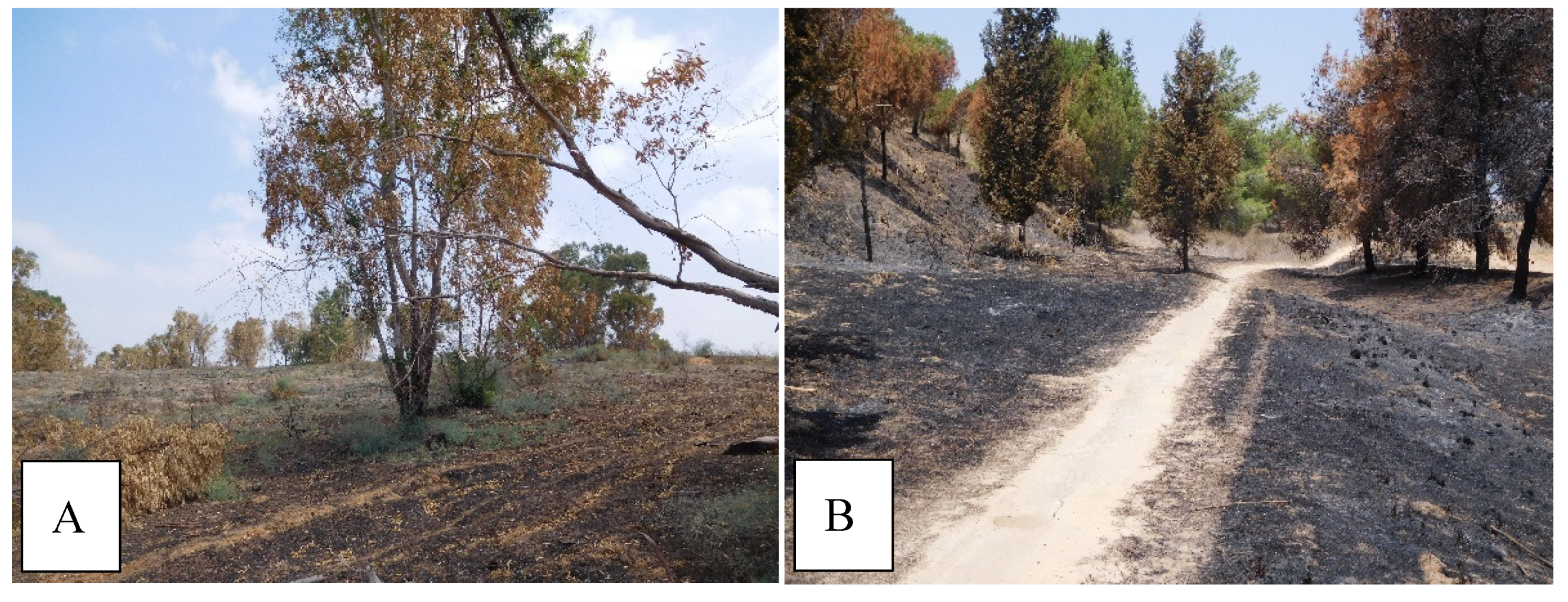
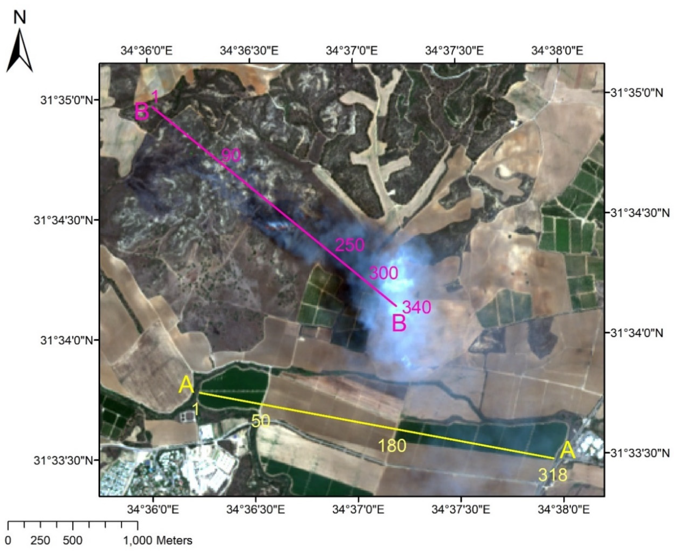
2.3. Ground Observations

Throughout the period of the Kit Terror, from 11 April to 22 December 2018, daily ground inspections were performed by the district JNF’s foresters, rangers, and firefighters. The affected areas were accurately mapped immediately after the active fire was extinguished using a designated mobile application. As a result, a two-class (burned/unburned) digital GIS database of fire scars was produced (Figure 2). This database was used as ground truth for validating the Earth observation’s algorithms.

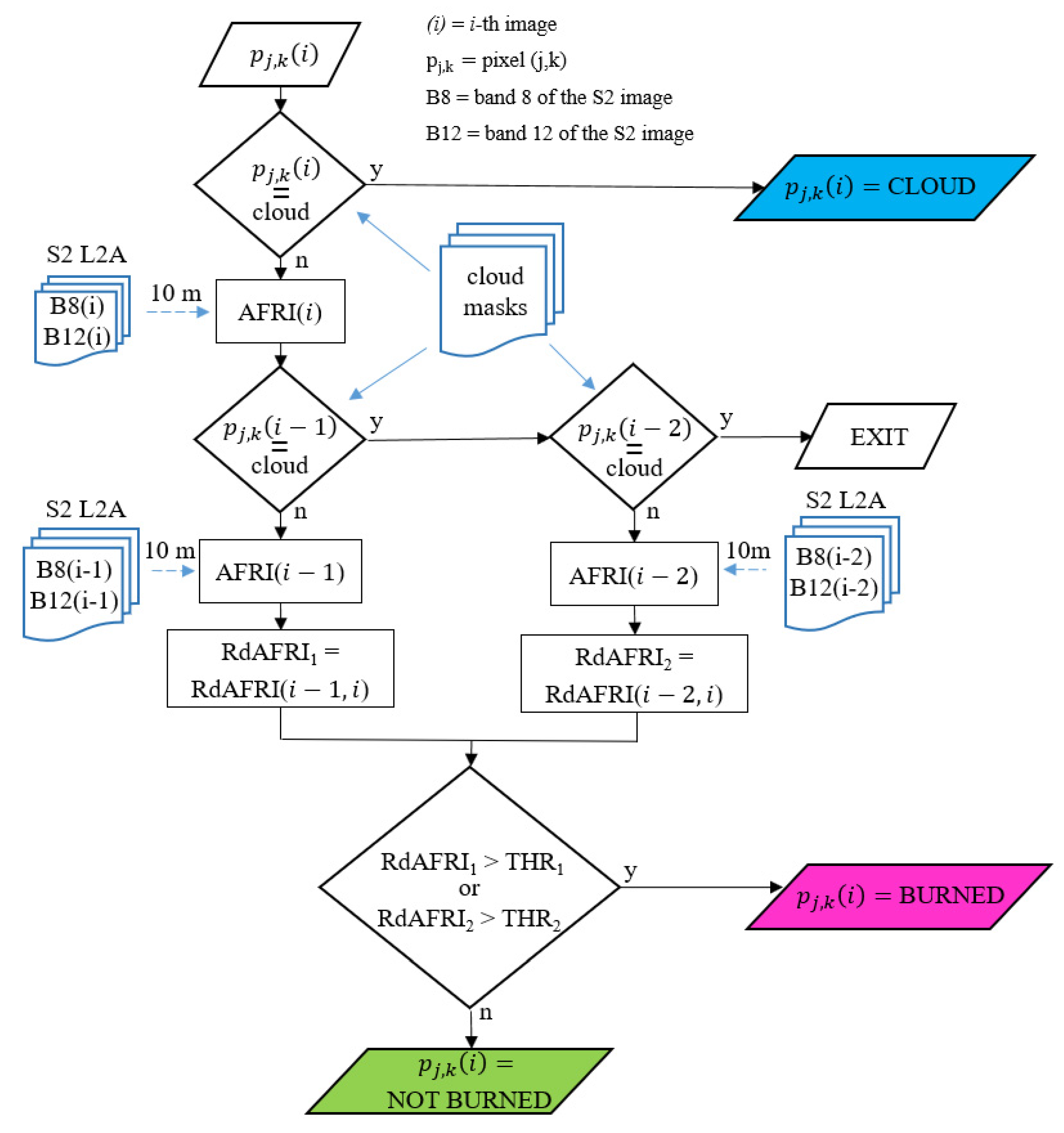
2.4. AFRI-Based Algorithms Development

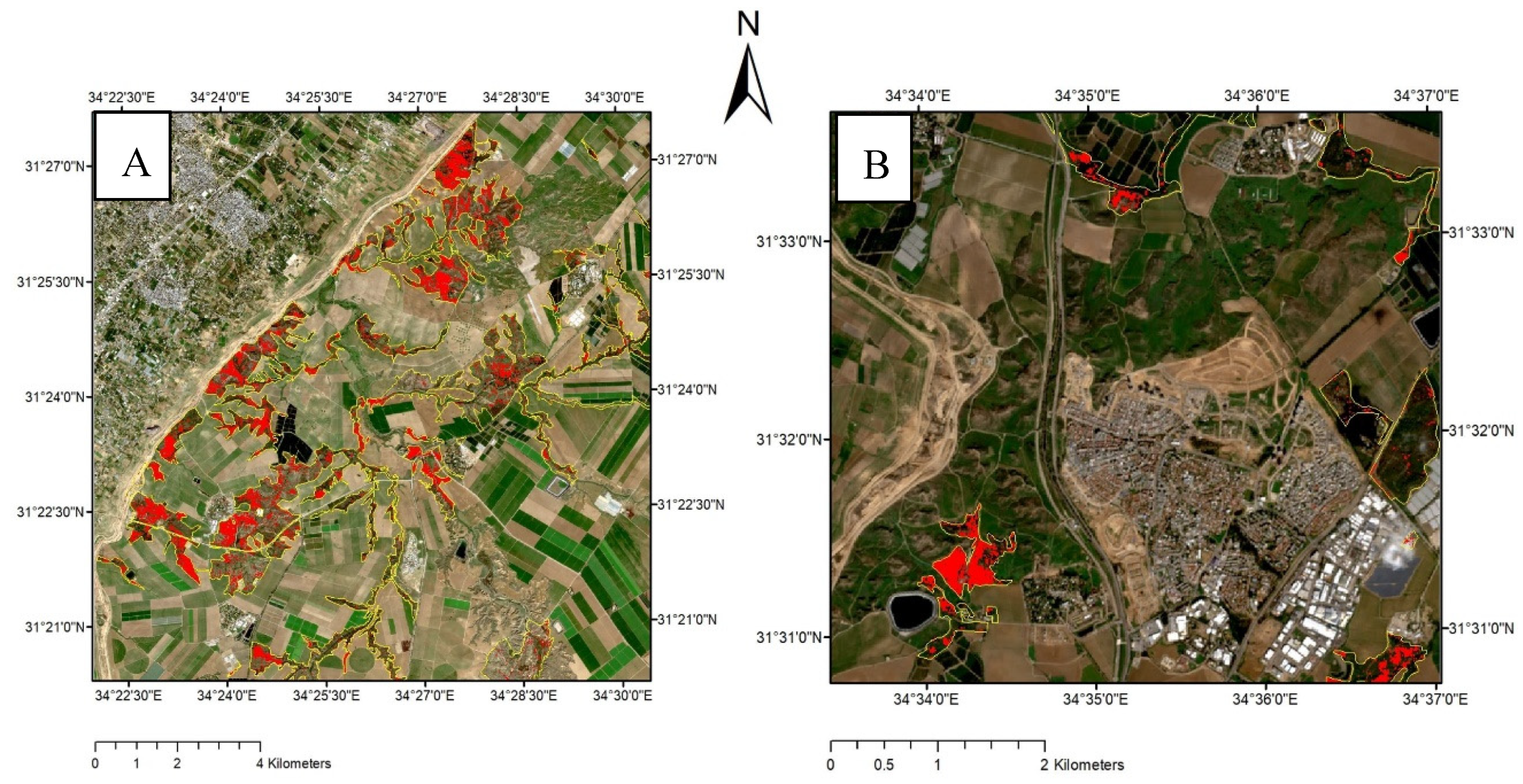
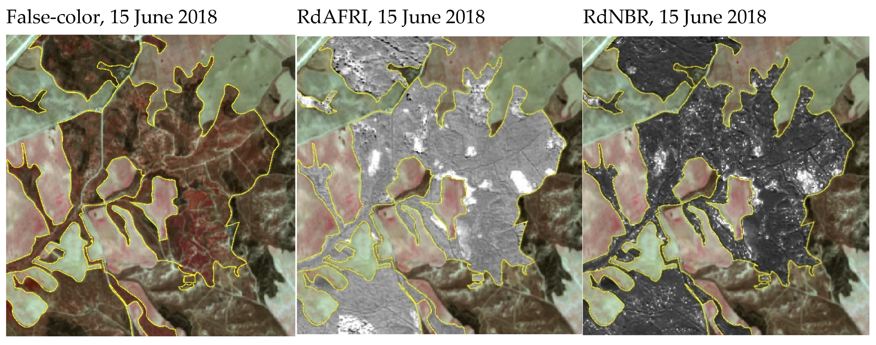
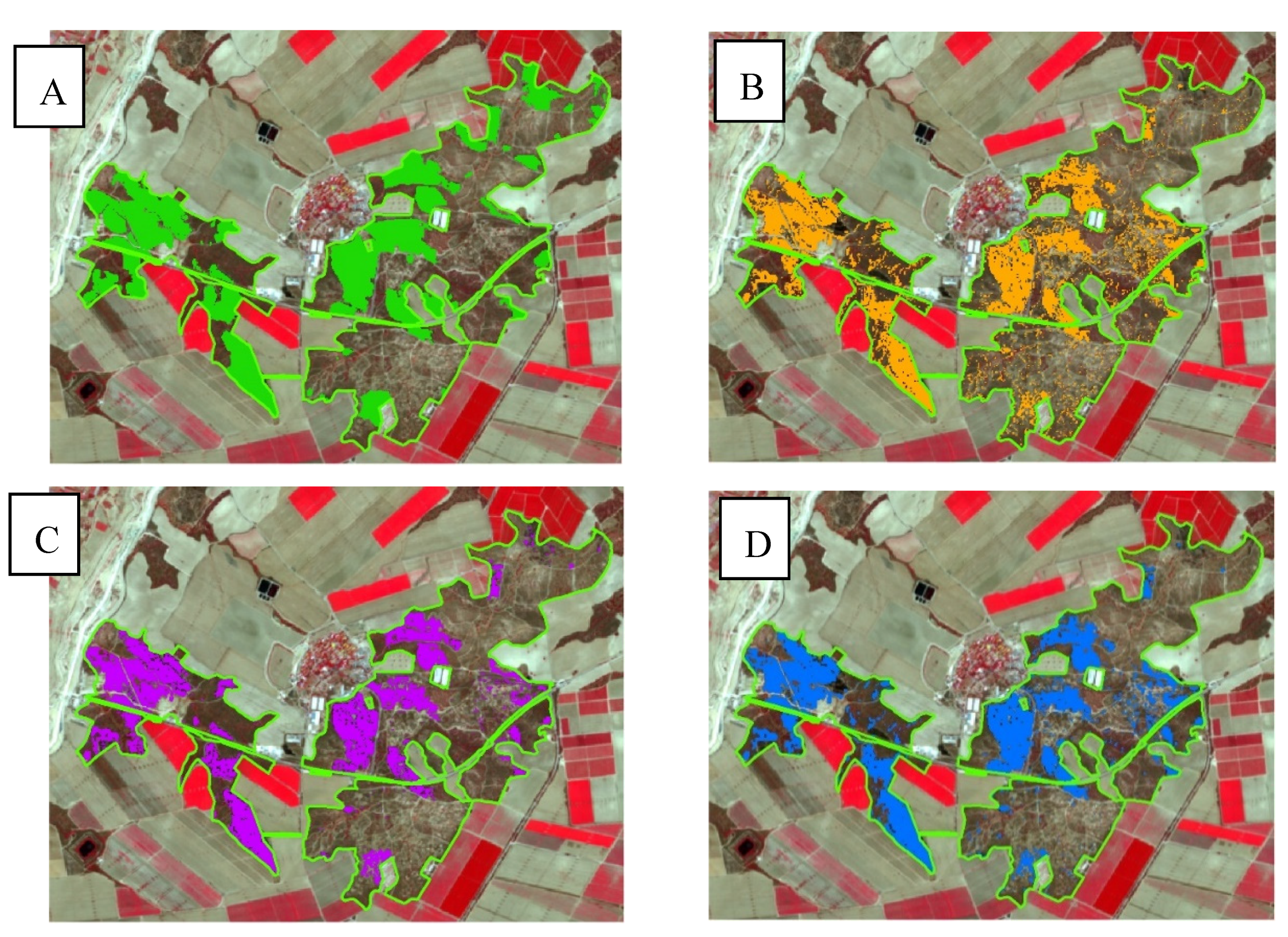
Similar to the procedures developed for the NBR-based set of algorithms, the most intuitive burned area-mapping indicator consists of an absolute change detection methodology obtained subtracting a post-fire AFRI image from a pre-fire AFRI image to derive the differenced AFRI (dAFRI):

$$\mathrm{dAFRI}={\mathrm{AFRI}}_{\mathrm{t}0}-{\mathrm{AFRI}}_{\mathrm{t}1}.$$

(6)

Then, the dAFRI, for two successive images collected in this study, can be formulated as:

$$\mathrm{dAFRI}\left(i-1, i\right)=\mathrm{AFRI}\left(i-1\right)-\mathrm{AFRI}\left(i\right),\mathrm{with}i=2,\cdots ,25$$

(7)

where (i) indicates the i-th image in the database. The dAFRI(i − 1, i) can present problems in the cases with low vegetation values for the image taken at (i − 1): the absolute change will be small, and the index will not be able to detect the burned area. In order to avoid this issue, similarly to the work proposed in [29,35], the relative differenced AFRI (RdAFRI) was defined as:

$$\mathrm{RdAFRI}\left(i-1, i\right)= \frac{\mathrm{dAFRI}\left(i-1, i\right)}{\sqrt{\left|\mathrm{AFRI}\left(i-1\right)\right|/1000}}.$$

(8)

Positive RdAFRI(i − 1, i) values represent a decrease in vegetation cover, while negative values represent an increase in vegetation cover. Therefore, the burned area can be easily identified when the relativized delta AFRI is greater than a threshold that has been chosen a priori.

The S2 Level-2A product contains vector cloud and cirrus masks that are created as a product of the atmospheric correction. These masks are used in this proposed methodology in order to compute the relative dAFRI only at the cloud-free pixels. The flowchart of the proposed classification algorithm is detailed in Figure 3. The indicator $p_{j,k}\left(i\right)$ represents the pixel located at row $j$ and column $k$ in the i-th image. The AFRI of the i-th image is computed from Equation (5), only for the cloud-free pixels, where ${\mathsf{\rho }}_{\mathrm{NIR}}$ and ${\mathsf{\rho }}_{\mathrm{SWIR}2}$ are the surface reflectance available at bands 8 and 12, respectively. Band 12 is resampled to 10 m in order to preserve the spatial resolution of band 8. The RdAFRI(i − 1, i) is computed only if the pixel $\left(j,k\right)$ of the (i − 1)-th image is also cloud-free. If not, the relative differenced AFRI is derived by the i-th and (i − 2)-th images, i.e., RdAFRI = RdAFRI(i − 2, i). Finally, the pixel $\left(j,k\right)$ is considered a burned surface if RdAFRI is greater than a fixed threshold. In this study, two thresholds were used: THR₁ for the relative differenced AFRI obtained by the i-th and (i − 1)-th images, and THR₂ for the relative differenced AFRI obtained by the i-th and (i − 2)-th images. With no loss of importance, the proposed methodology can be extended in order to manage more multi-temporal images, i.e., $p_{j,k}\left(i-3\right)$, $p_{j,k}\left(i-4\right)$, etc. In order to avoid that seasonal vegetation changes may be falsely detected as a burned area, a limited time expansion should be considered. The choice of the thresholds THR₁ and THR₂ is crucial in order to label a pixel as a burned or unburned area. An automated method, already used for wildfire burning and severity detection using Sentinel-2 images [21], is the Otsu threshold. This methodology distinguishes between background and foreground in imagery by creating two classes with minimal intraclass variance [46]. Alternatively, the value of the thresholds can also be chosen manually. In the current study, results were presented using both Otsu and manual thresholds.

Since the proposed classification algorithm is based on the RdAFRI values compared to a threshold, it is an applicative practice to quantify the noise degree of the relative difference AFRI images. For instance, the level of noise, denoted hereafter as a noise index (NI) of an image, can be computed from the following equation:

$$NI= \frac{{\sum }_{j=1}^m{\sum }_{k=1}^n{\sigma }_{j,k}^2}{N}$$

(9)

where ${\sigma }_{j,k}^2$ is the variance of the pixel $\left(j,k\right)$ computed in a neighborhood as a 3 × 3 matrix, $N$ is the total number of pixels, and $m \mathrm{and} n$ are the number of rows and columns, respectively.

3. Results

Throughout the study area, more than 1100 fires were counted by the JNF’s foresters, rangers, and firefighters. Ground observations revealed that most of the wildfires could be classified as ‘surface fire’, consuming mostly the understory grasses, shrubs, litter, and woody material lying on the ground [47]. Occasionally, the surface fire reached and injured the trunks of mature trees. In eucalyptus plots, damages were also observed in the lower foliage (Figure 4A). Pinus halepensis (Aleppo pine), the dominant pine species in the study area, is very sensitive to heat due to its relative thin bark and high amount of resin [48,49]. Therefore, many pines did not survive the surface fire (Figure 4B). Only the minority of the fires were characterized as ‘canopy fires’. In other species, such as acacia, mesquites, and tamarisk, the foliage was damaged, but the trees were recovered soon after the fire.

For comparing the performance of the NBR, NDVI, and AFRI indices, a section of the S2 Level-2A image obtained on 10 July 2018, close to the Gaza Strip border, is presented in Figure 5. The transects represent a common situation when smoke, at different intensities, covers a variety of substrates—cultivated, bare soils, fire scars, and more. The true-color composite image (RGB = 0.665, 0.56, 0.49 μm) shows the open fire (light-orange hue), the biomass burning smoke (white hue), as well as burned scars that are a few days old (dark surfaces). The three indices were produced at 10-m spatial resolution, according to Equations (1), (2), and (5), from the surface reflectance values along a cross-section of 2771 m (Figure 6, line A-A). This line was selected since it passes cultivated fields, bare soil, and was overcast by light smoke that characterized the entire region along the whole study period. This line is subdivided into several segments. From pixel 0 to 50 (and similarly from pixel 180 to 190) over the agricultural field where no smoke exists, the AFRI values accurately mimic those of the NDVI, but the NBR values are significantly lower. From pixel 50 to 180, over the bare soil, AFRI values are somehow higher than those of the NDVI. However, the NBR values are negative and much lower. From pixel 180 to 318, under the smoke, the AFRI values of the crops remain at the same high level as in the smoke-clear section, while both the NDVI and NBR produce low values.

Figure 7A shows the AFRI and NBR profiles along line B-B (Figure 5). This line was selected since it passes burned forest and cultivated fields. As already described in Figure 6, it can be noticed that the AFRI has a similar profile to NBR but with higher and positive values (Figure 7A). Furthermore, the latter index glides the zero value for the entire transect, expect in the crop area (from pixel 300 to 330). Figure 7B,C depict the profiles of dAFRI and dNBR and RdAFRI and RdNBR computed by Equations (6), (3), (8), and (4), respectively, between 5 July 2018 and 25 July 2018.

Figure 8 shows the false-color composite (RGB = 0.842, 0.665, 0.56 μm), the RdAFRI, and the RdNBR images for a portion of the study area obtained on 15 June 2018. The reference of the difference is the image acquired on 5 June 2018. It can be noticed that both RdAFRI and RdNBR emphasize the severity of the fire scars. The dark areas in the false-color composite are similar to the bright regions in the RdAFRI and RdNBR. However, in the RdNBR image, many pixels out of the burned area appear to have high index values that mislead any burned area interpretation. On the other hand, the RdAFRI image is smoother. Consequently, it is easier to select the threshold value (manually or from a systematics methodology) that flags a pixel as burned or not. By way of example, Figure 9 depicts the classification of the fire scars obtained by four levels of severity that are commonly used [29].

Table 2. Level of the noise index (NI) for RdAFRI and RdNBR images.

Image Date	NI RdAFRI	NI RdNBR
16 April 2018	0.022	4.317
11 May 2018	0.139	57.383
21 May 2018	0.055	15.943
5 June 2018	0.234	40.221
15 June 2018	0.088	51.396
25 June 2018	0.085	13.692
5 July 2018	0.087	9.678
10 July 2018	0.098	31.082
25 July 2018	0.294	16.423

details the values of NI for RdAFRI and RdNBR images as calculated from Equation (9) for selected dates and in the area with the lower burned severity index, i.e., RdAFRI <5.8. High values of NI mean high discrepancy between the index values with respect to their average values. Evidently, the noise degree in the RdNBR images is two orders of magnitude greater than the same calculated in the RdAFRI image.

Figure 10 and

Table 3. Temporal dynamics of the fire scars as observed by satellite images. THR stands for the threshold values.

Image i	Image Date in 2018	Clouds (%)	Burned Area (km2)	Additional Burned Area (km2)	Accumulated Burned Area (km2)	Ratio (%)	THR1	THR2
1	6 April	0.00	-	-	-	-	-	-
2	16 April	0.08	0.01	0.00	0.01	0.01	12	-
3	11 May	1.82	0.28	0.28	0.28	0.56	12	12
4	21 May	0.11	0.87	0.86	1.14	2.24	5.8	12
5	5 June	3.32	1.28	1.18	2.32	4.56	5.8	12
6	15 June	0.08	2.32	1.86	4.18	8.23	5.8	12
7	25 June	0.12	1.93	1.79	5.97	11.74	5.8	12
8	5 July	0.33	0.60	0.42	6.39	12.55	5.8	12
9	10 July	0.12	0.38	0.15	6.54	12.85	12	12
10	25 July	0.17	0.27	0.24	6.78	13.33	5.8	12
11	24 August	0.20	0.34	0.11	6.89	13.54	12	12
12	29 August	14.08	0.00	0.00	6.89	13.54	35	35
13	3 September	0.66	0.00	0.00	6.89	13.54	35	35
14	13 September	11.53	0.00	0.00	6.89	13.55	12	12
15	18 September	0.93	0.03	0.00	6.89	13.55	35	35
16	23 September	5.13	0.11	0.04	6.94	13.63	12	12
17	28 September	0.51	0.01	0.00	6.94	13.64	35	35
18	3 October	8.93	0.00	0.00	6.94	13.64	35	35
19	28 Oct0ber	0.26	0.01	0.00	6.94	13.64	35	35
20	2 November	0.25	0.07	0.03	6.96	13.69	12	12
21	12 November	7.92	0.01	0.01	6.97	13.70	35	35
22	17 November	4.09	0.00	0.00	6.97	13.70	35	35
23	12 December	1.59	0.01	0.01	6.98	13.72	12	12
24	17 December	4.03	0.03	0.03	7.01	13.78	12	12
25	22 December	4.21	0.01	0.01	7.02	13.79	12	12

depict the temporal dynamics of the fire scars as developed from the beginning of April to the end of December 2018, obtained by the algorithm proposed in Section 2.4.

Table 3 shows that the total burned area, within the JNF forests, is 7.02 km², which corresponds to 13.79% of the total JNF area. It is worth mentioning that in some cases, fires were set in areas that have already been set on fire and were previously counted as scars. For example, the fire on 10 July 2018 covered an area of 0.38 km², but only 0.15 km² were detected in new areas that were not burned before. The values of the thresholds THR1 and THR2 were chosen manually by visual inspection of the 24 S2 images.

For demonstration, Figure 11 presents the results of the proposed classification algorithm, i.e., AFRI, obtained for three successive S2 images, on 11 May, 21 May, and 5 June 2018. For each date, the false-color image (RGB = 0.842, 0.665, 0.56 μm) and the corresponding burned map image are provided.

As described in Section 2.3, a field campaign was conducted on 23 July 2018 in order to monitor the forest in the proximity of the Gaza Strip. The result of this campaign is vector data that locates all the burned territories inside the JNF areas, as defined in Figure 1. These ground-truth vector data were used to realize an accuracy assessment of the results obtained on 25 July 2018 by the proposed classification algorithm. Around 5000 points have been randomly distributed within all JNF areas, where each area has several points proportional to its relative area. The confusion matrix [50] that summarizes the classification performance is shown in

Table 4. Confusion matrix for the RdAFRI-based algorithm results.

		Algorithm Classification
Ground-Truth Data		Burned Area	Not Burned Area	Total	Accuracy
	Burned area	563	313	876	64%
	Not burned area	187	3875	4062	95%
	Total	750	4188	-	-
	Overall accuracy	75%	93%	-	90%

. The first column of the matrix indicates that 750 points have been classified by the algorithm as burned areas. Between them, 563 have been detected as “Burned areas” also by the ground-truth vector data, whereas 187 have been classified as “Not burned”. The positive predictive precision is 75%, and the negative predictive value is 93%, whereas the total accuracy is 90%.

Table 5. Statistic of the burned vegetation species on 22 December 2018.

Type of Vegetation	Burned Area (km2)	Burned Area (%)
Eucalyptus	3.44	16.36
Planted—coniferous	0.85	14.64
Planted—mixed coniferous and broadleaf	0.52	8.99
Planted—broadleaf, Israeli species	0.44	8.79
Planted—broadleaf, introduced species	0.74	10.71
Planted—other	0.01	3.07
Open landscape, bare soil	0.21	9.06
Planted—sparse	0.43	17.12
Orchard, bustan	0.00	0.85
Planted—shrubs	0.00	14.78
Desert shrubland	0.13	18.99
Garigue	0.18	30.40
Woodland	0.00	0.00

shows the statistics of the affected vegetation species in the JNF forest areas on 22 December 2018. For example, 16.36% of the eucalyptus trees were burned.

Figure 12 presents the spatial distribution of the accumulated fire scars (red pixels) in the JNF forests as for 22 December 2018 obtained by the proposed classification algorithm. Figure 13A,B is zoomed in to show the areas in more detail.

In order to compare the classification results obtained by the methodology presented in Section 2.4 with respect to an equivalent algorithm based on RdNBR, the Otsu threshold method was applied. A smaller area (5.3 km²) was considered with respect to the JNF forest presented in Figure 1. The area presents a uniform vegetation background (Figure 14). Among all 24 dates in the previous analysis, only 3 dates were selected: 5 June, 15 June, and 25 June 2018. The main reason is that in this area, the majority of the fire scars appears only on these 3 dates; therefore, the results could be compared with the ground measurement. Figure 14A–C show the ground measurements of the accumulated fire scars obtained by using the RdNBR-based algorithm and the RdAFRI-based algorithm, respectively. Since the RdNBR has high values even if ρ_NIR approaches ρ_SWIR2 (Figure 8), we have processed the classification results of the RdNBR-based algorithm with a majority filter tool in ArcGIS in order to replace pixel classification based on the majority of their contiguous neighboring pixels (Figure 14D).

Finally,

Table 6. Confusion matrix for the RdAFRI-based algorithm results for the area of Figure 14.

		Algorithm Classification
Ground-Truth Data		Burned Area	Not Burned Area	Total	Accuracy
	Burned area	309	151	460	67%
	Not burned area	49	980	1029	95%
	Total	358	1131	-	-
	Overall accuracy	86%	87%	-	87%

,

Table 7. Confusion matrix for the RdNBR-based algorithm results for the area of Figure 14.

		Algorithm Classification
Ground-Truth Data		Burned Area	Not Burned Area	Total	Accuracy
	Burned area	300	160	460	65%
	Not burned area	132	897	1029	87%
	Total	432	1057	-	-
	Overall accuracy	69%	84%	-	80%

and

Table 8. Confusion matrix for the RdNBR-based algorithm results with the majority filter tool for the area of Figure 14.

		Algorithm Classification
Ground-Truth Data		Burned Area	Not Burned Area	Total	Accuracy
	Burned area	310	152	462	67%
	Not burned area	85	942	1027	92%
	Total	395	1094	-	-
	Overall accuracy	78%	86%	-	84%

summarize the classification performances of the three methods. Around 1500 points have been randomly distributed within the study area of Figure 14. It can be noticed that the results obtained by RdAFRI are better than those obtained by RdNBR: the positive predictive precision is 86% and 69%, the negative predictive value is 87% and 84%, whereas the total accuracy is 87% and 80%, respectively. On the other hand, the RdNBR-based algorithm with a filter tool performs similarly to the proposed algorithm: the positive predictive precision is 78%, the negative predictive value is 86%, and the total accuracy is 84%.

4. Discussion

Wildfire is a complex issue, since it is related to changes in ecosystems, climate, land-use and land-cover, and management practices, and it also has many socio-economic implications [51,52]. Therefore, maps of fire scars provide valuable information for studying forestry, agriculture, and pedology, as well as climate change. Since Earth observation data are considered to be the most informative means for quantifying the scars, a large variety of space systems have been used for this purpose. Selecting the most appropriate satellite depends on several criteria. Obviously, for the continental to global scales, the large-swath satellites (e.g., NOAA-AVHRR, MODIS) are more suitable. In contrast, for a regional scale, high spatial resolution and narrow swath are preferable. The second criterion is the temporal resolution required for the specific application. The number of fires, burned areas, as well as derived environmental consequences, such as the amount of CO₂ emissions, are usually summed for a monthly, seasonally, or yearly period using the large-swath satellites. However, for fast response and accurate mapping (e.g., for insurance assessment), more frequent images from high-resolution satellites (e.g., Sentinel-2, VENµS, RapidEye, etc.) are essential. Thirdly, the most meaningful spectral index for enhancing the burned signal and differentiating severity levels needs to be identified. Concerning the study objectives, S2 was found to be a suitable satellite due to its characteristics—high spatial resolution of 10 m, high temporal resolution of about five days, and the SWIR bands for computing the AFRI.

AFRI was initially developed as an approved vegetation index. While NDVI is based on the red band that is more sensitive to atmospheric aerosols, AFRI relies upon the SWIR band(s) that enable the radiation to penetrate a polluted atmospheric column. Empirical linear relationships between the red and the SWIR2 band reveal that ρ_red ≈ 0.5ρ_SWIR2. Consequently, AFRI performs similar to NDVI, producing identical values under clear-sky conditions. However, under an opaque atmosphere influenced by biomass burning smoke, the NDVI values drop. Still, the AFRI continuously detects the real index values without the need for explicit correction for the aerosol effect.

In the current study, AFRI and its related algorithms were successfully used for delineating post-fire scars. While the AFRI values resembled the NDVI values when no smoke exists, the NBR values were significantly lower and even produced negative values over bare soils. Thoughtfully, the difference between positive and negative values enables the detection of the fire scars. In fact, beneath the smoke, the values of the NBR were as low as those of the NDVI. At the same time, the AFRI always kept high index values, disregarding even the light smoke that characterized the region during the nine months of the Kit Terror. The dAFRI and dNBR showed identical behavior both over unburned and burned areas. On the other hand, even if both successfully detected the burned area, the RdAFRI and RdNBR presented different behavior. Along the entire study area, the RdAFRI appeared to be smoother than the RdNBR, which was characterized by many noisy pixels. Mathematically, this phenomenon occurs when the NBR was computed on the pre-fire images—i.e., when the denominator of Equation (4) attains zero. As a result, some areas can be erroneously considered as fire scars, even if the dNBR value is low. Since the ${\mathsf{\rho }}_{\mathrm{SWIR}2}$ is multiplied by a factor of 0.5, this behavior does not occur in the RdAFRI index profile. The noise levels of the images produced by the RdAFRI algorithm were two orders of magnitude lower than the images produced by RdNBR. Consequently, by applying the RdAFRI, it is possible to identify manual thresholds for distinguishing among the four severity categories.

During the eight months of this study, the fire scars appeared in small areas, i.e., around 2% maximum of the whole forest area. The images of the entire area presented a different type of background (e.g., diverse types of vegetation). Consequently, the “automatic” Otsu threshold did not succeed in accurately classifying these small burned patches correctly concerning the whole study area. On the other hand, Otsu’s methodology worked very well if applied to images that circumscribe the burned areas, where the background was more uniform. In order to have an overview of the fire scars in the entire JNF forest, we opted for manual thresholds. These values were not unique for all the dates. The main reason is that the RdAFRI, but also the RdNBR, was sensible to the clouds over the pre and post-burned area. Even if the cloud mask product was used in order to avoid applying the algorithm at cloudy pixels, it appeared that many cloudy areas were not correctly flagged by the mask and were analyzed by the algorithm. Therefore, in the corresponding high cloud coverage images, a higher threshold was required in order to locate the burned area pixels concerning the cloud pixels correctly. Therefore, an accurate cloud mask product is a key factor for the accuracy of burned area mapping algorithms. For companion, the proposed algorithm was also implemented with the cloud screening and atmospheric correction procedure provided by the MACCS-ATCOR Joint Algorithm (MAJA) processor [43] that obtained similar results. In this regard, we admit that the main drawback of the proposed procedure (and also of the RdNBR) is determining the threshold level. This disadvantage can be overcome by more accurate filed calibration [35,53].

5. Conclusions

The study was derived by the need to map a sequence of more than 1100 wildfires that last nine months, partially over forest areas. Obviously, Earth observation is the preferable means for monitoring fire scars. Sentinel-2 was selected due to its considerable high spatial and temporal resolution, as well as suitable spectral bands. Naturally, two obstacles prevent accurate scar mapping. The first is the biomass burning smoke that continuously overcast the study area. This issue was solved by using the SWIR bands that can penetrate fine-mode atmospheric polluted aerosols. The AFRI spectral index, which uses the 2.1 µm band, is an atmospheric-resistant index that can observe vegetation through the smoke. Furthermore, its values closely resemble the NDVI values under clear-sky conditions, and it retains the same level of index values under smoke. In the latter regard, RdAFRI has proven to assess burned areas accurately as the equivalent RdNBR index with the advantage of not requiring sieved or filtering tools to remove erroneously fire scars pixel. Ground validation of the RdAFRI values reveals an overall accuracy of 90%. The RdAFRI enables one to distinguish among four severity categories; however, due to different cloud cover in two consecutive dates, an automatic determination of a threshold level was not possible. Therefore, two threshold levels were considered through visual inspection and manually assigned to each imaging date. It is concluded that the S2 AFRI-derived is the desirable means for calculating and mapping the spatio-temporal dynamics of the fire scars along with the statistics of the burned vegetation species. RdAFRI was found applicable, particularly when the area is affected by many fires that broke out at different places across the region and contaminated the air away from the fire center.

References

1. Williamson, G.J.; Bowman, D.M.J.S.; Price, O.; Henderson, S.B.; Johnston, F.H. A transdisciplinary approach to understanding the health effects of wildfire and prescribed fire smoke regimes. Environ. Res. Lett. 2016, 11, 125009. [Google Scholar] [CrossRef]
2. Wang, J.; Zhang, X. Investigation of wildfire impacts on land surface phenology from MODIS time series in the western US forests. ISPRS J. Photogramm. Remote Sens. 2020, 159, 281–295. [Google Scholar] [CrossRef]
3. Wulder, M.A.; White, J.C.; Alvarez, F.; Han, T.; Rogan, J.; Hawkes, B. Characterizing boreal forest wildfire with multi-temporal Landsat and LIDAR data. Remote Sens. Environ. 2009, 113, 1540–1555. [Google Scholar] [CrossRef]
4. Al-Dhief, F.T.; Sabri, N.; Fouad, S.; Latiff, N.M.A.; Albader, M.A.A. A review of forest fire surveillance technologies: Mobile ad-hoc network routing protocols perspective. J. King Saud Univ. Comput. Inf. Sci. 2019, 31, 135–146. [Google Scholar] [CrossRef]
5. Molaudzi, O.D.; Adelabu, S.A. Review of the use of remote sensing for monitoring wildfire risk conditions to support fire risk assessment in protected areas. S. Afr. J. Geomat. 2019, 7, 222. [Google Scholar] [CrossRef] [Green Version]
6. Szpakowski, D.M.; Jensen, J.L.R. A Review of the applications of remote sensing in fire ecology. Remote Sens. 2019, 11, 2638. [Google Scholar] [CrossRef] [Green Version]
7. Joyce, K.E.; Belliss, S.; Samsonov, S.V.; McNeill, S.; Glassey, P. A review of the status of satellite remote sensing and image processing techniques for mapping natural hazards and disasters. Prog. Phys. Geogr. Earth Environ. 2009, 33, 183–207. [Google Scholar] [CrossRef] [Green Version]
8. LeBlon, B. Monitoring forest fire danger with remote sensing. Nat. Hazards 2005, 35, 343–359. [Google Scholar] [CrossRef]
9. Ichoku, C.; Kaufman, Y.J.; Giglio, L.; Li, Z.; Fraser, R.H.; Jin, J.-Z.; Park, W.M. Comparative analysis of daytime fire detection algorithms using AVHRR data for the 1995 fire season in Canada: Perspective for MODIS. Int. J. Remote Sens. 2003, 24, 1669–1690. [Google Scholar] [CrossRef]
10. Filipponi, F. Exploitation of sentinel-2 time series to map burned areas at the national level: A Case Study on the 2017 Italy wildfires. Remote Sens. 2019, 11, 622. [Google Scholar] [CrossRef] [Green Version]
11. Sobrino, J.A.; Llorens, R.; Fernández, C.; Fernández-Alonso, J.M.; Vega, J.A. Relationship between soil burn severity in forest fires measured in situ and through spectral indices of remote detection. Forests 2019, 10, 457. [Google Scholar] [CrossRef] [Green Version]
12. Christopoulou, A.; Mallinis, G.; Vassilakis, E.; Farangitakis, G.; Fyllas, N.M.; Kokkoris, G.D.; Arianoutsou, M. Assessing the impact of different landscape features on post-fire forest recovery with multitemporal remote sensing data: The case of Mount Taygetos (southern Greece). Int. J. Wildland Fire 2019, 28, 521. [Google Scholar] [CrossRef] [Green Version]
13. Kaufman, Y.J.; Tucker, C.J.; Fung, I. Remote sensing of biomass burning in the tropics. J. Geophys. Res. Space Phys. 1990, 95, 9927–9939. [Google Scholar] [CrossRef]
14. Wang, Q.; Guo, F.; Hu, H.; Jin, S.; Su, Z. Estimation of gases emitted by forest fires based on remote sensing data. J. For. Res. 2015, 27, 369–378. [Google Scholar] [CrossRef]
15. Karnieli, A.; Kaufman, Y.J.; Remer, L.; Wald, A. AFRI—aerosol free vegetation index. Remote Sens. Environ. 2001, 77, 10–21. [Google Scholar] [CrossRef]
16. Vega-Garcia, C.; Chuvieco, E. Applying local measures of spatial heterogeneity to landsat-TM images for predicting wildfire occurrence in Mediterranean landscapes. Landsc. Ecol. 2006, 21, 595–605. [Google Scholar] [CrossRef]
17. Movaghati, S.; Samadzadegan, F.; Azizi, A. An agent-based approach for regional forest fire detection using modis data: A preliminary study in Iran. J. Indian Soc. Remote Sens. 2012, 41, 21–33. [Google Scholar] [CrossRef]
18. Yang, J.; Pan, S.; Dangal, S.; Zhang, B.; Wang, S.; Tian, H. Continental-scale quantification of post-fire vegetation greenness recovery in temperate and boreal North America. Remote Sens. Environ. 2017, 199, 277–290. [Google Scholar] [CrossRef]
19. Filipponi, F.; Valentini, E.; Xuan, A.N.; Guerra, C.A.; Wolf, F.; Andrzejak, M.; Taramelli, A. Global modis fraction of green vegetation cover for monitoring abrupt and gradual vegetation changes. Remote Sens. 2018, 10, 653. [Google Scholar] [CrossRef] [Green Version]
20. Fuller, D.O. Satellite remote sensing of biomass burning with optical and thermal sensors. Prog. Phys. Geogr. Earth Environ. 2000, 24, 543–561. [Google Scholar] [CrossRef]
21. Amos, C.; Petropoulos, G.P.; Ferentinos, K.P.; Feredinos, K. Determining the use of Sentinel-2A MSI for wildfire burning & severity detection. Int. J. Remote Sens. 2018, 40, 905–930. [Google Scholar] [CrossRef]
22. Navarro, G.; Caballero, I.; Silva, G.; Parra, P.-C.; Vázquez, Á.; Caldeira, R.M.A. Evaluation of forest fire on Madeira Island using Sentinel-2A MSI imagery. Int. J. Appl. Earth Obs. Geoinf. 2017, 58, 97–106. [Google Scholar] [CrossRef] [Green Version]
23. García-Llamas, P.; Suárez-Seoane, S.; Fernández-Guisuraga, J.M.; Fernández-García, V.; Fernández-Manso, A.; Quintano, C.; Taboada, A.; Marcos, E.; Calvo, L. Evaluation and comparison of Landsat 8, Sentinel-2 and Deimos-1 remote sensing indices for assessing burn severity in Mediterranean fire-prone ecosystems. Int. J. Appl. Earth Obs. Geoinf. 2019, 80, 137–144. [Google Scholar] [CrossRef]
24. Veraverbeke, S.; Harris, S.; Hook, S. Evaluating spectral indices for burned area discrimination using MODIS/ASTER (MASTER) airborne simulator data. Remote Sens. Environ. 2011, 115, 2702–2709. [Google Scholar] [CrossRef]
25. Van Leeuwen, W.J.D.; Casady, G.M.; Neary, D.G.; Bautista, S.; Alloza, J.A.; Carmel, Y.; Wittenberg, L.; Malkinson, D.; Orr, B.J. Monitoring post-wildfire vegetation response with remotely sensed time-series data in Spain, USA and Israel. Int. J. Wildland Fire 2010, 19, 75. [Google Scholar] [CrossRef]
26. Key, C.; Benson, N.C. The Normalized Burn Ratio (NBR): A Landsat TM Radiometric Measure of Burn Severity. Available online: http://nrmsc.usgs.gov/research/ndbr.htm (accessed on 25 August 2020).
27. Miller, J.D.; Yool, S.R. Mapping forest post-fire canopy consumption in several overstory types using multi-temporal Landsat TM and ETM data. Remote Sens. Environ. 2002, 82, 481–496. [Google Scholar] [CrossRef]
28. Escuin, S.; Navarro, R.; Fernandez, P. Fire severity assessment by using NBR (Normalized Burn Ratio) and NDVI (Normalized Difference Vegetation Index) derived from LANDSAT TM/ETM images. Int. J. Remote Sens. 2007, 29, 1053–1073. [Google Scholar] [CrossRef]
29. Miller, J.D.; Thode, A.E. Quantifying burn severity in a heterogeneous landscape with a relative version of the delta Normalized Burn Ratio (dNBR). Remote Sens. Environ. 2007, 109, 66–80. [Google Scholar] [CrossRef]
30. Parks, S.A.; Dillon, G.K.; Miller, C. A new metric for quantifying burn severity: The relativized burn ratio. Remote Sens. 2014, 6, 1827–1844. [Google Scholar] [CrossRef] [Green Version]
31. Furniss, T.J.; Kane, V.R.; Larson, A.J.; Lutz, J.A. Detecting tree mortality with Landsat-derived spectral indices: Improving ecological accuracy by examining uncertainty. Remote Sens. Environ. 2020, 237, 237. [Google Scholar] [CrossRef]
32. Meddens, A.J.; Kolden, C.A.; Lutz, J.A. Detecting unburned areas within wildfire perimeters using Landsat and ancillary data across the northwestern United States. Remote Sens. Environ. 2016, 186, 275–285. [Google Scholar] [CrossRef]
33. Hislop, S.; Haywood, A.; Jones, S.; Soto-Berelov, M.; Skidmore, A.; Nguyen, T.H. A satellite data driven approach to monitoring and reporting fire disturbance and recovery across boreal and temperate forests. Int. J. Appl. Earth Obs. Geoinf. 2020, 87, 102034. [Google Scholar] [CrossRef]
34. Manzo-Delgado, L.L.; López-García, J. Spatial and temporal analyses of burned areas 1998, 2003 and 2015 in Montes Azules biosphere reserve, Chiapas, Mexico. Bosque 2020, 41, 11–24. [Google Scholar] [CrossRef]
35. Hudak, A.T.; Morgan, P.; Bobbitt, M.J.; Smith, A.M.S.; Lewis, S.A.; Lentile, L.B.; Robichaud, P.R.; Clark, J.T.; McKinley, R.A. The relationship of multispectral satellite imagery to immediate fire effects. Fire Ecol. 2007, 3, 64–90. [Google Scholar] [CrossRef]
36. Jia, J.; Wang, Y.; Zhuang, X.; Yao, Y.; Wang, S.; Zhao, D.; Shu, R.; Wang, J. High spatial resolution shortwave infrared imaging technology based on time delay and digital accumulation method. Infrared Phys. Technol. 2017, 81, 305–312. [Google Scholar] [CrossRef]
37. Kaufman, Y.; Remer, L. Detection of forests using mid-IR reflectance: An application for aerosol studies. IEEE Trans. Geosci. Remote Sens. 1994, 32, 672–683. [Google Scholar] [CrossRef]
38. Ben-Zeev, E.; Karnieli, A.; Agam, N.; Kaufman, Y.; Holben, B. Assessing vegetation condition in the presence of biomass burning smoke by applying the Aerosol-free Vegetation Index (AFRI) on MODIS images. Int. J. Remote Sens. 2006, 27, 3203–3221. [Google Scholar] [CrossRef]
39. Hirschberger, P. Forests Ablaze: Causes and Effects of Global Forest Fires; WWF: Vaud, Switzerland, 2016; p. 108. [Google Scholar]
40. Le Page, Y.; Oom, D.; Silva, J.; Jönsson, P.; Pereira, J.M.C. Seasonality of vegetation fires as modified by human action: Observing the deviation from eco-climatic fire regimes. Glob. Ecol. Biogeogr. 2010, 19, 575–588. [Google Scholar] [CrossRef]
41. Short, K.C. Spatial Wildfire Occurrence Data for the United States, 1992–2015, 4th ed.; Rocky Mountain Research Station: Fort Collins, CO, USA, 2017. [Google Scholar]
42. Balch, J.K.; Bradley, B.A.; Abatzoglou, J.; Nagy, R.C.; Fusco, E.J.; Mahood, A.L. Human-started wildfires expand the fire niche across the United States. Proc. Natl. Acad. Sci. USA 2017, 114, 2946–2951. [Google Scholar] [CrossRef] [Green Version]
43. Baird, R.A. Pyro-terrorism—The threat of arson-induced forest fires as a future terrorist weapon of mass destruction. Stud. Confl. Terror. 2006, 29, 415–428. [Google Scholar] [CrossRef]
44. Copernicus Open Access Hub. Available online: https://scihub.copernicus.eu/ (accessed on 25 August 2020).
45. Gatti, A.; Naud, C.; Castellani, C.; Carriero, F. Sentinel-2 Products Specification Document; Thales Alenia Space: Cannes, France, 2018. [Google Scholar]
46. Otsu, N. A threshold selection method from gray-level histograms. IEEE Trans. Syst. Man Cybern. 1979, 9, 62–66. [Google Scholar] [CrossRef] [Green Version]
47. Graham, R.T.; McCaffrey, S.; Jain, T.B. Science Basis for Changing Forest Structure to Modify Wildfire Behavior and Severity USDA Forest Service, Rocky Mountain Research Station, General Technical Report RMRS-GTR-120. Available online: https://digitalcommons.usu.edu/cgi/viewcontent.cgi?article=1161&context=barkbeetles (accessed on 25 August 2020).
48. Palmero-Iniesta, M.; Domènech, R.; Molina-Terrén, D.; Espelta, J.M. Fire behavior in Pinus halepensis thickets: Effects of thinning and woody debris decomposition in two rainfall scenarios. For. Ecol. Manag. 2017, 404, 230–240. [Google Scholar] [CrossRef]
49. Ne’Eman, G.; Goubitz, S.; Nathan, R. Reproductive traits of Pinus halepensis in the light of fire—a critical review. Plant Ecol. 2004, 171, 69–79. [Google Scholar] [CrossRef]
50. Ting, K.M. Confusion Matrix. In Encyclopedia of Machine Learning and Data Mining; Springer Science and Business Media LLC: Berlin/Heidelberg, Germany, 2017; p. 260. [Google Scholar]
51. Doerr, S.H.; Santin, C. Global trends in wildfire and its impacts: Perceptions versus realities in a changing world. Philos. Trans. R. Soc. B Boil. Sci. 2016, 371, 20150345. [Google Scholar] [CrossRef]
52. Cochrane, M.A. Burning questions about ecosystems. Nat. Geosci. 2019, 12, 86–87. [Google Scholar] [CrossRef]
53. Veraverbeke, S.; Hook, S.; Harris, S. Synergy of VSWIR (0.4–2.5 μm) and MTIR (3.5–12.5 μm) data for post-fire assessments. Remote Sens. Environ. 2012, 124, 771–779. [Google Scholar] [CrossRef]
Figure 1. Sentinel-2 image of the study area. The Jewish National Fund (JNF) forests are marked in yellow.
Remotesensing 12 02753 g001
Figure 2. Map of the ground observations and respective data of the monthly expanded of the burned areas within the Jewish National Fund (JNF) forest.
Remotesensing 12 02753 g002
Figure 3. Flowchart of the pixel-based classification algorithm for burned area mapping based on the relative differenced Aerosol-Free Vegetation Index (RdAFRI) and multi-temporal Sentinel-2 Level-2A products.
Remotesensing 12 02753 g003
Figure 4. Surface fire affecting the trunks and lower foliage in eucalyptus (A) and burning pine trees (B).
Remotesensing 12 02753 g004
Figure 5. A true-color (RGB = 0.665, 0.56, 0.49 μm) daily surface reflectance image of the Israeli territory on 10 July 2018. The open fire appears in a light-orange hue, the burn scars are dark, and the smoke is a white hue.
Remotesensing 12 02753 g005
Figure 6. AFRI, Normalized Difference Vegetation Index (NDVI), and Normalized Burn Ratio (NBR) values along the cross-section embedded on the image on 10 July 2018. The x-axis numbers represent the pixels’ distance along line A–A in accordance with Figure 5.
Remotesensing 12 02753 g006
Figure 7. AFRI and Normalized Burn Ratio (NBR) (A); dAFRI and dNBR (B); and RdAFRI and relative dNBR (RdNBR) (C) values along the cross-section B-B embedded on Figure 5.
Remotesensing 12 02753 g007
Figure 8. False-color image with the corresponding RdAFRI and RdNBR images on 15 June 2018.
Remotesensing 12 02753 g008
Figure 9. Classification of the fire scars’ severity levels on the RdAFRI image of 15 June 2018.
Remotesensing 12 02753 g009
Figure 10. Temporal dynamics of the fire scars as observed by the Sentinel-2 images.
Remotesensing 12 02753 g010
Figure 11. False-color (RGB = 0.842, 0.665, 0.56 μm) images with the corresponding burned maps obtained by the proposed AFRI algorithm from 11 May 2018 to 5 June 2018. Blue pixels indicate clouds, whereas pink pixels indicate burned areas (only within the JNF study polygons, delineated by the yellow lines). It can be noticed that some burned areas can be identified comparing two successive false-color images (black area).
Remotesensing 12 02753 g011
Figure 12. Spatial distribution of the accumulated fire scars (in red) in the JNF forests for 22 December 2018.
Remotesensing 12 02753 g012
Figure 13. Magnified areas of the accumulated fire scars in parts of Figure 12. (A) Southern insert; (B) northern insert.
Remotesensing 12 02753 g013
Figure 14. False-color (RGB = 0.842, 0.665, 0.56 μm) images with (A) ground observations (green pixels); (B) accumulated fire scars based on RdNBR (orange pixels); (C) accumulated fire scars based on RdAFRI (pink pixels); and (D) accumulated fire scars based on RNBR and majority filter (blue pixels). Images are from 5 June 2018 to 25 June 2018.
Remotesensing 12 02753 g014