Integration of Geospatial Tools and Multi-source Geospatial Data to Evaluate the Tropical Forest Cover Change in Central America and Its Methodological Replicability in Brazil and the DRC

Abstract

Satellite monitoring of forests plays a relevant role in the agendas of tropical countries, mainly in the framework of international negotiations to implement a mechanism that ensures a reduction in global CO₂ emissions from deforestation. An efficient way to approach this monitoring is to avoid duplication of efforts, generating products in a regional context that are subsequently adopted at the national level. In this effort, you should take advantage of the different data sources available by integrating geospatial tools and satellite image classification algorithms. In this research, a methodological framework was developed to generate cost-efficient national maps of forest cover and its dynamics for the countries of Central America, and its scalability and replicability was explored in the Democratic Republic of the Congo (DRC) and the State of Pará in Brazil. The maps were generated from Landsat images from the years 2000, 2012, and 2017. New geoprocessing elements have been incorporated into the digital classification procedures for satellite images, such as the automated extraction of training samples from secondary sources, the use of official national reference maps that respond to nationally adopted forest definitions, and automation of post-classification adjustments incorporating expert criteria. The applied regional approach offers advantages in terms of reducing costs and time, as well as improving the consistency and coherence of reports at different territorial levels (regional and national), reducing duplication of efforts and optimizing technical and financial resources. In Central America, the percentage of forest area decreased from 44% in 2000 to 38% in 2017. Average deforestation in the 2000–2012 period was 197,443 ha/year and that of 2012–2017 was 332,243 ha/year. Average deforestation for the complete period 2000–2017 was 264,843 ha/year. The tropical forests in both the State of Pará, Brazil, and the DRC have decreased over time.

1. Introduction

Satellite monitoring, as a tool to support decision making aimed at halting forest destruction, has been prioritized in the last decade under the mechanism known by its initials REDD+ (reducing emissions from deforestation and forest degradation). REDD+ is an initiative of the United Nations Framework Convention on Climate Change (UNFCCC) that requires the implementation of consistent, transparent, and robust national monitoring systems, maintaining a balance between the costs required for monitoring and the resources that are necessary to allocate for the execution of direct actions to reduce deforestation. One of the ways to reduce monitoring costs is to take advantage of the economy of scale to generate useful global or regional protocols and products at the national level. The objective of the research was to develop and apply a theoretical–methodological framework (as a technical input in the decision-making process to curb deforestation) in order to cost-efficiently prepare national cartography on forest cover, which is temporarily consistent, scalable at the supranational level for the Central American region, and applicable to other tropical regions.

1.1. State of the Research Field

Since the end of the 20th century, different initiatives have taken place to generate forest maps in the Central American countries and/or the region as a whole. STEP (System for Terrestrial Ecosystem Parameterization), developed from the Global Observation for Forest Cover and Land Dynamics (GOFC/GOLD), was one of the first vegetation mapping experiences at a regional level in Central America with Advanced Very High Resolution Radiometer (AVHRR) images (from 1 km spatial resolution [1].

In 2000, the Central American Commission for Environment and Development (CCAD) produced the Map of Ecosystems of Central America based on the visual interpretation of Landsat images and field verifications, reconnaissance flights, and the participation of experts in ecology from the region [2]. In 2003, Giri and Jenkins [3] generated a regional forest cover map for Central America and Mexico in which, using Moderate Resolution Imaging Spectroradiometer (MODIS) of 500 m resolution, nine types of vegetation cover were identified. The most recent regional cartography is the 2010 Central American Map of Land Use and Cover, prepared by the Center for Water in the Humid Tropics for Latin America and the Caribbean (CATHALAC, Panama City, Panama) from MODIS images of 500 m resolution, which applied a methodology of supervised classification for the identification of sixteen land cover classes [4].

At the national level in Central America, most of the forest cover maps have been generated from Landsat images [5,6,7,8,9]. However, in an effort to improve the scale of forest mapping and land cover, national forest type maps were developed with 5 m resolution RapidEye satellite imagery, acquired in 2012 in Honduras [10], Costa Rica [11], Guatemala [12], Panamá [13], El Salvador and Nicaragua [14]. More recently, in 2019, Guatemala published a new map of forest cover for the year 2016 and dynamics 2010–2016 [15]; in Panama that same year, a diagnosis on the coverage of forests and other wooded land was prepared, which was based on a 2019 update of the forest map [16]. Other countries, such as Honduras [17] and Nicaragua [14], have also reported information on the dynamics of forest cover at REDD+ reference levels submitted by the countries to the United Nations Framework Convention on Climate Change (UNFCCC, New York, NY, USA).

Among the forest cover classification algorithms, the most widely used in Central America is the maximum-likelihood classifier (MLC). It was used to generate the series of forest cover maps with Landsat images from 2001, 2006, and 2010 in Guatemala [6,7]; in Belize, for the elaboration of the forest map series of 1980, 1989, 1994, 2000, 2004, 2010 and 2012 from Landsat images [8,18], and to generate the map of forest types with RapidEye images from 2014 in Honduras [10] and from 2015 in Guatemala [12]. At the regional level, MLC was applied to prepare the 2010 Central American Map of Land Use and Cover [4].

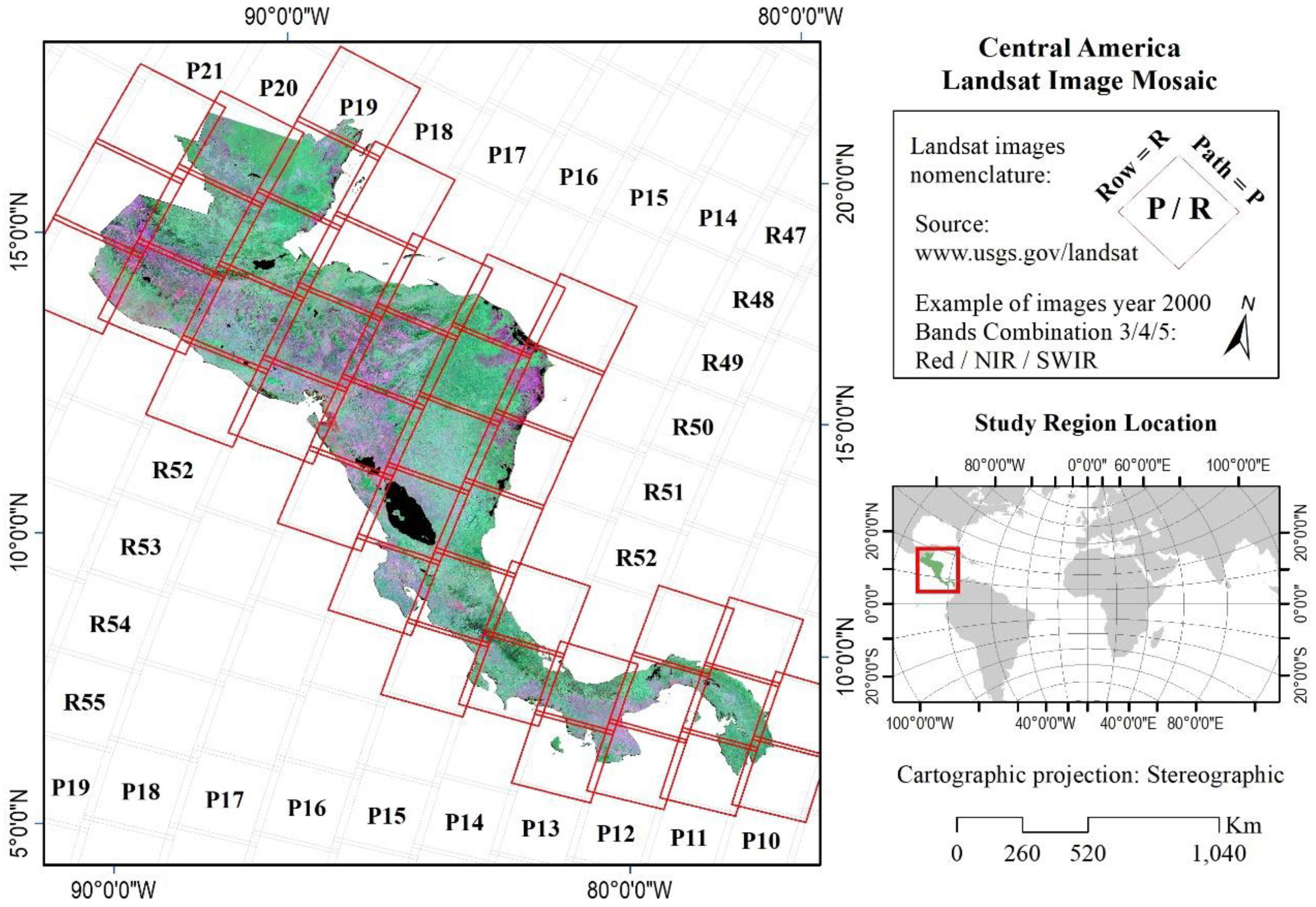
Currently, taking advantage of improvements in data processing, it is now possible to access from the cloud a large number of orthorectified and geometrically corrected images under the global land survey standard [19], and derived from new policies of open access to satellite data by this means, it is possible to access the complete historical catalog of Landsat images [20]. The development of new radiometric standardization methods is also currently allowing the generation of global, regional, national, and subnational image mosaics [21], ensuring uniform access to spatially and temporally standardized satellite images [22].

The progressive consolidation of the cloud as a paradigm for the delivery of information and services is facilitating the management and massive analysis of large volumes of satellite data, making traditional analysis scene by scene less feasible and leading some authors to talk about “the end of per scene analysis” [23]. In this context, the University of Maryland, together with Google and the United States Geological Survey (USGS, Reston, VA, USA), taking advantage of the benefits of cloud computing, implemented a project to generate worldwide mapping of the loss and gains of tree cover, with a resolution of 30 m using Landsat images [24].

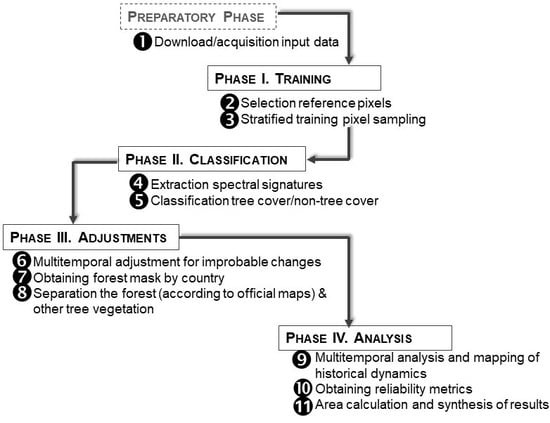
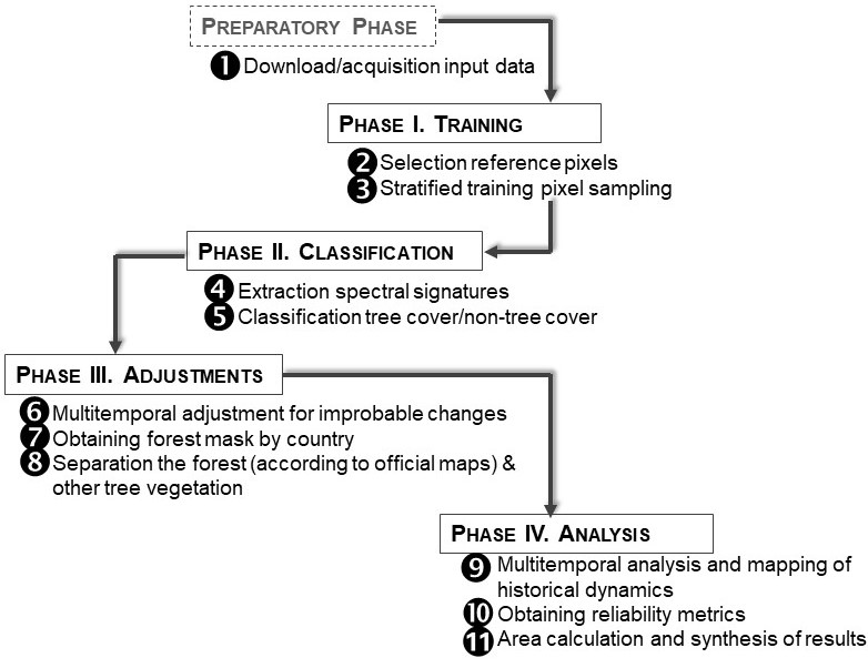
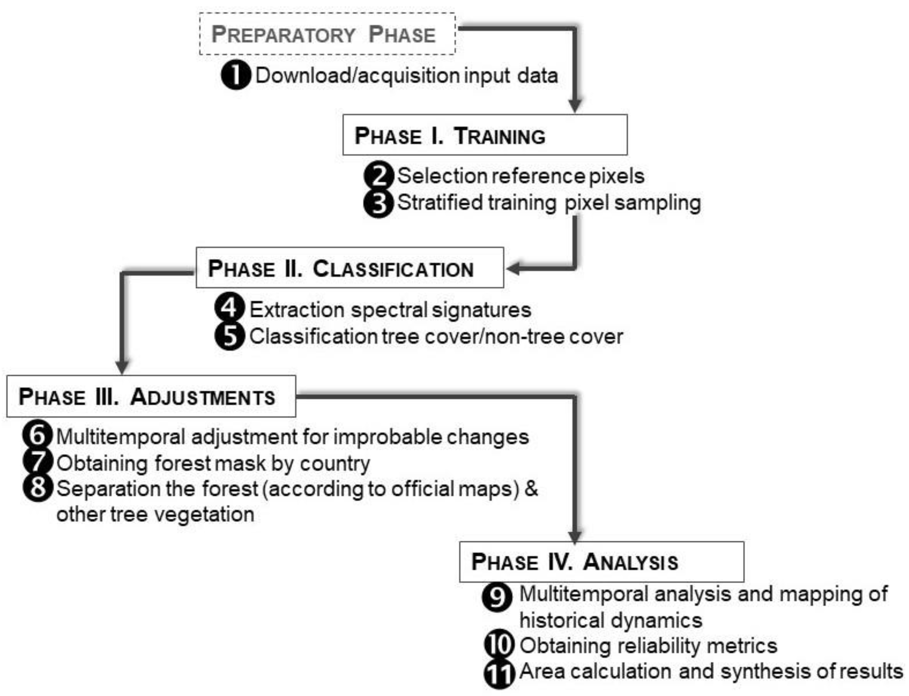
The objective of this article is to develop a theoretical–methodological framework for the cost-efficient elaboration of national cartography on forest cover in Central America, temporarily consistent and scalable at the supranational level. Workflows are proposed to reduce the time usually taken by the satellite image classification process, automating the capture of training samples from multisource data and incorporating automated human decision adjustments post-classification based on expert criteria.

1.2. Contextual Framework

The Central American region is a relatively small portion of territory, where different vegetation types coexist, such as humid forest, dry forest, coniferous forest, mangrove swamps, and even some specifically localized niches of xerophytic scrub and flooded vegetation [2]. It is for this reason that it has become a key region for conducting studies on the dynamics of tropical forests that can be extrapolated to other sites with similar characteristics.

However, most of the mapping of forest cover generated in Central America from remote sensor data have been prepared separately for each country applying different criteria [6,7,8,9,10,11,12,13,14,15,16], making it difficult to obtain a complete and comparable vision for the entire region. Tropical countries share similarities in vegetation types [2], and this facilitates the generation and use of data in a shared way, such as training samples, mosaics of satellite images, and classification protocols. In this context, as part of this research, the requirement to develop and apply a methodology that allows the generation of national maps of forest cover using a regional framework was addressed.

There are several challenges in digital image classification processes for the mapping of forest cover; some are related to errors in pixel assignment in the mapping carried out in Central America and are corrected by making a visual sweep across the map and recoding the pixels to assign them to the right classes [6,7]. The problem derived from this practice is that it is difficult to replicate, since most of the time the decisions and criteria used by the interpreter when making the corrections are not recorded, and if they are documented, it is not ensured that each one of the pixels is visited by visual sweep with these types of inconsistencies corrected. In this study, it is proposed to develop a method that allows the introduction of human decisions based on expert judgment to include them within the same classification model, so that they are applied automatically.

Another challenge is related to the fact that not all the pixels classified as tree cover in a classification process are necessarily forest according to the national definitions adopted. A pixel in one country may correspond to forest, but the same type of vegetation detected in that pixel in another country could be considered non-forest. For example, in some countries early secondary vegetation is considered secondary forest, but in other countries that same type of vegetation is classified as secondary non-forest vegetation. In this sense, this research considers the application of national forest masks to separate what proportion of the pixels classified as tree cover correspond to forest according to national definitions.

In summary, the problem addressed in this study focuses on addressing the challenges facing tropical countries and, specifically, those of Central America to generate data on forest cover dynamics under the same theoretical–methodological framework replicable in a context supranational regional (regions made up of several countries). At the same time, it seeks to reduce the effort, cost, and time involved in preparing national forest mapping in small countries, such as Central America, by developing a method that can be replicated in countries and/or large areas, also with limited financial and human resources. The replication potential and scalability of the methodology was explored to be applied to other tropical regions of greater territorial extension.

2. Materials and Methods

2.1. Study Region

This study was in the Central American region, located within the intertropical zone, specifically between 7°30′ and 18°30′ of north latitude and 76°30′ and 92°30′ of west longitude, including seven countries: Belize, Costa Rica, El Salvador, Guatemala, Honduras, Nicaragua, and Panama. Although Central America is the smallest of the tropical regions, four of the five tropical and subtropical biomes of the world are represented in it, according to the World Map of Terrestrial Ecoregions [25]. Central America has an area of approximately 523,000 km².

2.2. Target Period

The years of study were selected based on data availability. The year 2000 (T₁) is the initial date from which the 30 m resolution data from the Global Forest Change Project (GFC) on canopy cover percentage and annual tree cover losses are available [24]. The year 2012 (T₂) corresponds to the date in which the Central American national maps of forests and/or land cover were prepared with high resolution images (5 m). Finally, 2017 (T₃) corresponds to the last available annual mosaic of satellite images that was accessed at the time of applying the algorithms and the classification model developed in this research. From the logic of monitoring, reporting and verification (MRV) of the REDD+ mechanism, the historical period [T₁–T₂–T₃] analyzed in this study simulates the reference level against which the impact will be measured in terms of REDD+ actions that countries will implement to reduce their emissions from deforestation. In this sense, T₃₊₁ represents the first monitoring event to compare the increase or decrease in the change rate in terms of deforestation, which in this case, corresponds to 2018.

Although the analysis period in this study was defined based on the available information, in future studies it is expected to carry out analyzes with longer periods. The reason is that deforestation where a forest mass changes from forest to non-forest, can be mapped in short periods, but the detection of forest gains requires longer periods.

2.3. Data

A global set was formed that, combined with local data, was the base input for the classification processes implemented.

2.3.1. Worldwide Data

The main worldwide data source used was the 30 m resolution raster dataset generated by the Department of Geographical Sciences (GEOG) at the University of Maryland (UMD) under the Global Forest Change Project (GFC) [24]. From GFC, the treecover2000 and treecover2010 raster were obtained, which contain the percentage of the tree canopy at the pixel level of 30 m for the years 2000 and 2010, respectively. Furthermore, the annual Landsat image mosaics were obtained from GFC for the years 2000, 2012, and 2017, as well as the lossyear data of annual tree canopy losses that occurred during the period 2001–2017. The coverage loss data in 2018 (T₃₊₁) was obtained from the lossyear raster of GFC version 1.6 (https://earthenginepartners.appspot.com/science-2013-global-forest/download_v1.6.html). The Landsat mosaics obtained correspond to multispectral image composites generated by calculating the median value of pixels with less cloudiness in the year in question. For it, all the images available in the worldwide Landsat catalog were reviewed taking advantage of the cloud processing possibilities offered by the Google Earth Engine platform. [24]. The mosaics of the years 2000, 2012, and 2017 of Central America correspond, in each year, to 42 scenes from the worldwide catalog of Landsat images from which the best quality pixels in terms of cloudiness were selected (Figure 1).

2.3.2. National Data

The second source of data used in this study was the 2012 national forest and/or cover and/or land-use maps generated in Guatemala, El Salvador, Honduras, Nicaragua, Costa Rica, and Panama from RapidEye satellite images of 5 m resolution. In the case of Belize, the 2012 forest cover map generated from Landsat 7 ETM + images was used.

2.4. Methodological Framework

The general methodological framework applied consisted of a preparatory phase and 4 development phases that involved a total of 11 steps (Figure 2). All training and classification geoprocesses were automated using the ArcPy geoprocessing library package, implemented within the Python programming language in ArcGIS 10.5 and modeled with the ArcGIS Model Builder tool.

2.4.1. Training Samples

A procedure has been developed to automate the extraction of training samples, selecting the pixels that in the different sources had been assigned to some type of forest cover, as an indicator that they had remained unchanged throughout the period analyzed.

The GFC raster treecover2000 (T₁) and treecover2010 (≈T₂) were used as global data sources to make the selection of the reference pixels. Pixels that indicated a canopy cover of less than 10% in both rasters were assigned to the non-arboreal without change class, and pixels that indicated a canopy cover of more than 30% were assigned to the arboreal without change class (The applied canopy percentage thresholds were established in such a way as to capture the extremes of coverage percentage for each class, excluding the intermediate values (between 10–30%). The objective was to select the most representative unchanged pixels (pure pixels), that is, those that during the analyzed period had remained in the same range as those defined thresholds.).

For T₃ (2017), no tree canopy cover percentage data were found, but under the same logic of selecting only pixels without change for the entire period analyzed, all those that coincided with the tree canopy loss raster (lossyear) were excluded from the arboreal without change raster of the period [T₁–T₃]. Subsequently, the national forest coverage maps of 5 m resolution generated in Central America for the year 2012 were incorporated into the process. These maps were resampled to a resolution of 30 m, the same as the GFC data, and were reclassified into three classes of arboreal vegetation (broadleaf, coniferous, and mangrove) and two classes of non-arboreal vegetation (other land and water). The final selection consisted of extracting the arboreal and non-arboreal pixels that coincided with these same classes in the national forest cover maps, obtaining as a result the reference pixel raster. The training sample used was obtained from the selection of 0.1% of the total pixels of this raster.

The selection was made by applying a stratified random sampling design proportional to the number of reference pixels per country within each class. In this sense, the first stratum was represented by the country and the second by the different arboreal and non-arboreal classes. In this way, the size of the sample in each class was proportional to the number of pixels that class represented in each country within the reference pixel raster.

By corresponding the pixels of the training sample to sites that remained unchanged throughout the analyzed period, they could be applied to classify the Landsat images of any of the years that are located within the analyzed time horizon (T₁–T₃), hence it was given the name of multitemporal training pixel sample.

2.4.2. Classification Process

The process of digital classification of forest cover was applied separately for each country, which meant using national image mosaics for T₁, T₂, and T₃ and, consequently, also generating spectral signature files for each country and year. The multitemporal training pixel sample and spectral values of the image bands were used to extract the spectral signatures for the broadleaf, coniferous, and mangrove arboreal vegetation classes, as well as for other land and water (non-arboreal classes). Spectral information was obtained from the red wavelength band, the near infrared band (NIR), and two short-wave infrared (SWIR) bands. The red and NIR bands are suitable for the differentiation of vegetation compared to other types of land cover, and the SWIR bands provide additional information for the differentiation of different moisture content of vegetation (Figure 3).

The spectral signatures generated were used to classify the image mosaics from which they were extracted, resulting in three raster maps with arboreal and non-arboreal cover classes for T₁, T₂, and T₃ for each country. The maximum-likelihood classifier algorithm with Bayesian inference was used in the classification process, based on previous studies in which significant improvements were found in the assignment of pixels to a certain class [26,27]. This algorithm considers in the calculation the probability that each pixel belongs to certain class, but in this case including estimating a prior occurrence probability proportional to the total number of training pixels within each class and each country.

The maximum-likelihood classifier in its basic version assumes equal a priori probabilities for each class as follows in Equation (1):

$$p({\mathrm{X}}_k|i)=\frac{1}{{\left(2\mathsf{\pi }\right)}^{\mathrm{n}/2}{\left|{\mathrm{V}}_i\right|}^{1/2}}\exp [-1/2({\mathrm{X}}_k-{\mathrm{u}}_i{)}^{\mathrm{T}}{\mathrm{V}}_i^{-1}({\mathrm{X}}_k-{\mathrm{u}}_i)$$

(1)

where:

• p(X_k|i) = probability function for a pixel X_k as a member of class i
• n = number of spectral bands
• X_k = spectral values vector for the pixel in all bands
• u_i = mean vector for class i over all pixels
• V_i = variance–covariance matrix for class i
• (X_k − u_i)^T V_i⁻¹ (X_k − u_i) = spectral distance between the pixel value and the centroid value of class i

With the above formula the pixels are assigned to the class with which it has the highest a posteriori probability of membership. However, by incorporating the Bayesian approach, a priori probabilities were calculated (proportional to the sample size of each class) as follows in Equation (2):

$$L(i|{\mathrm{X}}_k)=\frac{P_{i}p\left(X_k|i\right)}{{\displaystyle \sum _{r=1}^t{P}_{r}p\left(X_k|r\right)}}$$

(2)

where:

• L(i|X_k) = a posteriori probabilities of a pixel X_k belonging to class i
• i = class number
• t = total number of classes
• P_i = a priori probability of membership of class i

When implementing the above formula in the classification algorithm, the sum of the a posteriori probabilities of each pixel is equal to 1.

2.4.3. Post-Classification Adjustment for Improbable Changes

In multitemporal analysis of forest cover changes, two or more years are compared to determine the vectors of change that, in descriptive terms, translate into gains, losses, and no-change. However, due to errors in assigning pixels to the different classes, in many cases there can be multitemporal inconsistencies in changes between forest types; not logical changes from the point of view of forest ecology [2]. These changes have been called multitemporal improbable changes in this study; for example, it is unlikely that the change of a pixel went from broadleaf to coniferous between 2012 and 2017; that one was classified in 2000 as mangrove and broadleaf in 2012 and 2017, or that a pixel in 2000 was assigned to coniferous, in 2012 to mangrove, and in 2017 to broadleaf.

A thorough review would surely allow us to find logical explanations for each case and make the necessary adjustments and corrections. However, this is complicated when, as in this case, there are millions of pixels, with all their possible variations, that would have to be revised. In Central American forest mapping, it has been common practice to make these corrections from a visual analysis of the map, with the identification, recoding, and assignment of erroneous pixels to the correct class, according to the interpreter’s judgment [10,11,12]. However, this practice is difficult to replicate, since in most cases, the decisions and criteria used are not documented. Furthermore, visual analysis does not always ensure that all pixels with inconsistencies are visited and corrected.

In order to have a structured base of the registry of adjustment for multitemporal improbable changes, a triple-entry table was constructed to identify all the possible combinations that would result from comparing the classes in the maps of each year T₁, T₂, and T₃ (

Table 1. Adjustment for multitemporal improbable changes.

Map T1	Map T2	Map T3
		ARBBROADLEAF	ARBCONIFEROUS	ARBMANGROVE	noARB	Water
ARBBROADLEAF	ARBBROADLEAF	B-B-B	B-B-B	B-B-B	B-B-NA	B-B-B
	ARBCONIFEROUS	B-B-B	C-C-C	M-M-M	C-C-NA	C-C-C
	ARBMANGROVE	B-B-B	C-C-C	M-M-M	M-M-NA	M-M-M
	noARB	B-NA-B	C-NA-C	M-NA-M	B-NA-NA	B-NA-NA
	Water	B-B-B	C-C-C	M-M-M	B-NA-NA	W-W-W
ARBCONIFEROUS	ARBBROADLEAF	B-B-B	C-C-C	M-M-M	B-B-NA	B-B-B
	ARBCONIFEROUS	C-C-C	C-C-C	C-C-C	C-C-NA	C-C-C
	ARBMANGROVE	B-B-B	C-C-C	M-M-M	M-M-NA	M-M-M
	noARB	B-NA-B	C-NA-C	M-NA-M	C-NA-NA	C-NA-NA
	Water	B-B-B	C-C-C	M-M-M	C-NA-NA	W-W-W
ARBMANGROVE	ARBBROADLEAF	B-B-B	C-C-C	M-M-M	B-B-NA	B-B-B
	ARBCONIFEROUS	B-B-B	C-C-C	M-M-M	C-C-NA	C-C-C
	ARBMANGROVE	M-M-M	M-M-M	M-M-M	M-M-NA	M-M-M
	noARB	B-NA-B	C-NA-C	M-NA-M	M-NA-NA	M-NA-NA
	Water	B-B-B	C-C-C	M-M-M	M-NA-NA	W-W-W
noARB	ARBBROADLEAF	NA-B-B	NA-C-C	NA-M-M	NA-B-NA	NA-B-NA
	ARBCONIFEROUS	NA-B-B	NA-C-C	NA-M-M	NA-C-NA	NA-C-NA
	ARBMANGROVE	NA-B-B	NA-C-C	NA-M-M	NA-M-NA	NA-M-NA
	noARB	NA-NA-B	NA-NA-C	NA-NA-M	NA- NA-NA	NA- NA-NA
	Water	NA-NA-B	NA-NA-C	NA-NA-M	NA- NA-NA	W-W-W
Water	ARBBROADLEAF	B-B-B	C-C-C	M-M-M	NA-B-NA	W-W-W
	ARBCONIFEROUS	B-B-B	C-C-C	M-M-M	NA-C-NA	W-W-W
	ARBMANGROVE	B-B-B	C-C-C	M-M-M	NA-M-NA	W-W-W
	noARB	NA-NA-B	NA-NA-C	NA-NA-M	NA- NA-NA	W-W-W
	Water	W-W-W	W-W-W	W-W-W	W-W-W	W-W-W

Nomenclature: ARB = arboreal vegetation; ARB_BROADLEAF/B = broadleaved arboreal vegetation; ARB_CONIFEROUS/C = coniferous arboreal vegetation; ARB_MANGROVE/M = mangrove arboreal vegetation; noARB/NA = non-arboreal; Water/W = water bodies.

). In the direction of the rows, the fields contain the references of the combinations of the classes between T₁ and T₂ and in the direction of the columns the combination with T₃. Each field resulting from the combination contains the sequence of classes to which the pixels must be assigned in each year in the event that such combination is observed, considering in those assignments the adjustments that, in expert criteria, should be made when improbable changes are detected.

To associate the adjustment table with the raster data (join) and perform the reclassifications at the pixel level, numerical coding was established that served as the unique identifier (ID) of each combination, defining in each case whether they corresponded to probable multitemporal changes or unlikely. For the latter, the table contains the classes to which the pixels in T1, T2, and T3 should be reassigned after adjustment. The code was formed by multiplying the numerical identifiers of each class (1–5) in T1, T2, and T3, respectively, by 1000, 100, and 10 and then adding them arithmetically. This same process was applied using map algebra to the corresponding raster data to generate the ID at the pixel level. In this way, the unique code of the combinations was represented in both tables, which were joined by the combination of units of thousands, hundreds, and tens.

In order to automate the adjustments, the multitemporal adjustment criteria for improbable changes were incorporated into the workflow of the classification process. With the implementation of this workflow, the classifications of the years 2000 (T₁), 2012 (T₂), and 2017 (T₃) were obtained in each country with built-in multitemporal adjustments.

2.4.4. Post-Classification Adjustment for Separation of Forest from Another Tree Vegetation

Central American countries use varied definitions of forest to respond to the different reporting needs of forest area and its changes. Conceptually this implies that not all pixels classified as tree cover in an automated regional classification process are necessarily forest according to the national definitions adopted in each country. This is the main reason why the ranking algorithm runs separately for each country.

In this context, the application of national forest masks was considered, which, generated for a base year, would allow us to identify in the pixels classified as tree cover those corresponding to forest according to definitions and national criteria. In subsequent years of monitoring, these masks would be used to determine if gains or losses cover come from areas classified as forest or from non-forest areas in the base year.

The pixels named forest in the official national maps were grouped and reclassified to obtain a binary raster (forest and non-forest) that became the forest mask of each country in T₂ (M_T2). Then the cover maps T₁, T₂, and T₃ were combined with the forest mask M_T2, and from the combinations, the map of each year was adjusted using the expert criteria collected in

Table 2. Separation of forest from other tree vegetation in T₁ and T₂.

Input Rasters				Combination Code (ID)	Adjustment		Change Vector [T1–T2] *
Tree Cover T1	Loss [T1–T2]	Forest Mask MT2	Tree Cover T2		Map T1 Adjusted	Map T2 Adjusted
Arboreal (10)	Loss (1000)	Non-Forest (100)	Arboreal (7)	1117	Forest (1)	Oth. Veg. (2)	1→2
			Non-Arboreal (8)	1118	Forest (1)	Non-T. Veg. (3)	1→3
		Forest (200)	Arboreal (7)	1217	Forest (1)	Forest (1)	1→1
			Non-Arboreal (8)	1218	Forest (1)	Non-T. Veg. (3)	1→3
	Non-Loss (2000)	Non-Forest (100)	Arboreal (7)	2117	Oth. Veg. (2)	Oth. Veg. (2)	2→2
			Non-Arboreal (8)	2118	Oth. Veg. (2)	Non-T. Veg. (3)	2→3
		Forest (200)	Arboreal (7)	2217	Forest (1)	Forest (1)	1→1
			Non-Arboreal (8)	2218	Oth. Veg. (2)	Non-T. Veg. (3)	2→3
Non-Arboreal (20)	Loss (1000)	Non-Forest (100)	Arboreal (7)	1127	Oth. Veg. (2)	Oth. Veg. (2)	2→2
			Non-Arboreal (8)	1128	Oth. Veg. (2)	Non-T. Veg. (3)	2→3
		Forest (200)	Arboreal (7)	1227	Oth. Veg. (2)	Oth. Veg. (2)	2→2
			Non-Arboreal (8)	1228	Oth. Veg. (2)	Non-T. Veg. (3)	2→3
	Non-Loss (2000)	Non-Forest (100)	Arboreal (7)	2127	Non-T. Veg. (3)	Oth. Veg. (2)	3→2
			Non-Arboreal (8)	2128	Non-T. Veg. (3)	Non-T. Veg. (3)	3→3
		Forest (200)	Arboreal (7)	2227	Non-T. Veg. (3)	Forest (1)	3→1
			Non-Arboreal (8)	2228	Non-T. Veg. (3)	Non-T. Veg. (3)	3→3

* Change Vector Nomenclature: (1) = forest, (2) = other tree vegetation, (3) = without tree vegetation.

and

Table 3. Separation of forest from other tree vegetation in T₃.

Input Raster Classes			Combination Code (ID)	Map T2 Adjusted	Map T3 Adjusted	Change Vector [T2–T3] *
Loss [T2–T3]	Map T2 Adjusted	Tree Cover T3
Loss (1000)	Forest (10)	Arboreal (7)	1017	Forest (1)	Oth. Veg. (2)	1→2
		Non-Arboreal (8)	1018	Forest (1)	Non-T. Veg. (3)	1→3
	Oth. Veg. (20)	Arboreal (7)	1027	Oth. Veg. (2)	Non-T. Veg. (3)	2→3
		Non-Arboreal (8)	1028	Oth. Veg. (2)	Non-T. Veg. (3)	2→3
	Non-T. Veg. (30)	Arboreal (7)	1037	Non-T. Veg. (3)	Non-T. Veg. (3)	3→3
		Non-Arboreal (8)	1038	Non-T. Veg. (3)	Non-T. Veg. (3)	3→3
Non-Loss (2000)	Forest (10)	Arboreal (7)	2017	Forest (1)	Forest (1)	1→1
		Non-Arboreal (8)	2018	Forest (1)	Non-T. Veg. (3)	1→3
	Oth. Veg. (20)	Arboreal (7)	2027	Oth. Veg. (2)	Oth. Veg. (2)	2→2
		Non-Arboreal (8)	2028	Oth. Veg. (2)	Non-T. Veg. (3)	2→3
	Non-T. Veg. (30)	Arboreal (7)	2037	Non-T. Veg. (3)	Oth. Veg. (2)	3→2
		Non-Arboreal (8)	2038	Non-T. Veg. (3)	Non-T. Veg. (3)	3→3

* Change Vector Nomenclature: (1) = forest, (2) = other tree vegetation, (3) = without tree vegetation.

.

The first four columns of Table 2 contain the numeric codes of the input rasters: initial tree cover in T1, first period losses [T1–T2], forest mask MT2, and final tree cover in T2. In the fifth column, the codes of the possible combinations corresponding to the arithmetic sum of the individual numeric codes of the input rasters are included, which also corresponds to the unique identifier of the combination (ID). The adjustments applied to T1 and T2 are indicated in the sixth and seventh columns, and finally, the eighth column contains the change vector [T1–T2] resulting from the adjustment. The final class codes were adjusted/reclassified and indicated in the change vectors are: (1) = forest; (2) = other tree vegetation and (3) = without tree vegetation.

A similar procedure was used to adjust and reclassify in T3 using Table 3, with the difference that, in this, the forest mask and the initial coverage in T2 were replaced by the adjusted raster obtained as a result of the application of Table 2 (second column). Subsequently, as in the previous case, the different input rasters were combined and adjustments were made in T3 according to what is indicated in Table 3.

2.4.5. Mapping of Forest Cover Change Dynamics

Once the adjusted rasters for T₁, T₂, and T₃ were obtained, they were integrated into a single file in order to analyze the multitemporal dynamics of forest cover. A reference table of all possible combinations (

Table 4. Categories assignment of forest cover change dynamics to the combined raster [T₁–T₂–T₃].

Map T1		Map T2		Map T3
				1	2	3
				Forest	Other Tree Vegetation	Without Tree Vegetation
100	Forest	10	Forest	111	112	113
		20	Other tree vegetation	121	122	123
		30	Without tree vegetation	131	132	133
200	Other tree vegetation	10	Forest	211	212	213
		20	Other tree vegetation	221	222	223
		30	Without tree vegetation	231	232	233
300	Without tree vegetation	10	Forest	311	312	313
		20	Other tree vegetation	321	322	323
		30	Without tree vegetation	331	332	333

Combination codes related to the categories of forest cover change dynamics: (1) Stable forest = 111; (2) Forest gain = 211, 311; (3) Other tree vegetation =222; (4) Exchange (non-forest) = 221, 223, 231, 232, 233, 321, 322, 323, 331, 332; (5) Without tree vegetation =333; (6) Forest loss (1st period) = 121, 122, 123, 131, 132, 133; (7) Forest loss (2nd period) = 112, 113; (8) Exchange (forest) = 212, 213, 312, 313.

) was generated in order to automate within the workflow the assignment of forest cover change dynamics categories to the combined raster [T₁–T₂–T₃].

By implementing the adjustments for improbable multitemporal changes, by forest mask and multitemporal analysis, new attributes associated with the dynamics of change of the analyzed period were generated that enriched the classification of forest cover in each year. The next step was to transfer these attributes to the individual forest cover maps of each year analyzed, obtaining the following classes in each: (1) stable late or mature forest; (2) early secondary forest; (3) other stable non-forest tree vegetation; (4) exchange (forest and non-forest); (5) deforested; (6) without tree vegetation (

Table 5. Assignment of the attributes of the forest cover change dynamics to the maps of each year.

Code	Forest Cover Change Dynamics	Class T1	Class T2	Class T3
1	Stable forest	Forest SLM (1)	Forest SLM (1)	Forest SLM (1)
2	Forest gain	Non-T. Veg. (6)	Forest ES (2)	Forest ES (2)
3	Other tree vegetation	Other SNF (3)	Other SNF (3)	Other SNF (3)
4	Exchange (non-forest)	Exchange (4)	Exchange (4)	Exchange (4)
5	Without tree vegetation	Non-T. Veg. (6)	Non-T. Veg. (6)	Non-T. Veg. (6)
6	Forest loss (1st period)	Forest SLM (1)	Deforest (5)	Deforest (5)
7	Forest loss (2nd period)	Forest SLM (1)	Forest SLM (1)	Deforest (5)
8	Exchange (forest)	Exchange (4)	Exchange (4)	Exchange (4)

Forest SLM (1) = stable late or mature forest|Forest ES (2) = early secondary forest|Other SNF (3) = other stable non-forest tree vegetation|Exchange (4) = exchange (forest and non-forest) | Deforest (5) = deforested | Non-T. Veg. (6) = without tree vegetation.

). In this way, in each annual map, in addition to knowing the current forest cover area, the dynamics of the forest can also be interpreted spatially in terms of losses, gains, stability, and exchange. Losses refer to the deforestation class and gains to the recent secondary forest class. Stability corresponds to the classes of stable late or mature forest and other stable non-forest tree vegetation. For its part, the exchange refers to the temporary changes between tree vegetation and without tree vegetation but also includes areas that are detected as forest in one period but are subsequently deforested in the next.

2.4.6. Validation

In this study, different cartographic products have been generated, but for validation purposes, only the cover maps in the forest/non-forest classes were evaluated, to determine the level of correspondence between the maps obtained and those identified in a validation sample of 5000 points randomly distributed throughout the region. The evaluation of each sampling point was implemented by visual interpretation of high-resolution satellite images available circa 2000 (Mainly Google Earth) and circa 2012 (Mainly RapidEye). The year 2017 was not evaluated as it was not possible to obtain a high-resolution image coverage for the entire region circa that year.

In the visual interpretation sequence, the first source of verification was the high-resolution images available on the Google Earth platform, and in the event of not finding a high-resolution image available (due to cloudiness or that did not exist), the next source were the RapidEye images (available for 2012). In cases where a high-resolution image was not available for the validation point, the visual interpretation was performed on Landsat image mosaics generated on the Google Earth Engine platform.

The evaluation of each validation point consisted of reviewing whether or not they intersected treetops, and when this was the case, it was interpreted as forest and otherwise as non-forest. After interpreting the 5000 points using a confusion matrix, the overall reliability, the sampling error, and the respective confidence intervals were calculated. Reliability was assessed separately by country and at the regional level.

2.5. Scaling Up and Methodology Replica in Other Tropical Regions

The entire territory of the Democratic Republic of the Congo (DRC) and the State of Pará, Brazil, were selected to explore the scaling up potential and replication of the methodology (Figure 4).

In the zones where the methodology was replicated, the same temporality of the data for Central America was used, that is, 2000–2012 for [T₁–T₂] and 2012–2017 for [T₂–T₃]. In the State of Pará, for the reference map of the types of coverage, two sources based on Landsat images were obtained: (1) the 2012 land-use and coverage map, obtained from the 1.0 collection of the MapBiomas-Amazonía project (https://amazonia.mapbiomas.org/) and (2) the TerraClass 2012 map of the Legal Amazon generated by INPE (https://www.terraclass.gov.br/). For the Democratic Republic of the Congo, there was no access to land cover data for the entire country with resolutions equal to less than 30 m, but there was a product of vegetation types generated for the Congo basin for the year 2012 based on MERIS images of 300 m resolution obtained from the Central African Forest Observatory data portal (https://www.observatoire-comifac.net/). It was decided to use this map to explore how the model results behave by integrating lower resolution input data to generate the forest mask and the extraction of spectral signatures. The other input data were obtained from the same global data sources described for Central America from the Department of Geographical Sciences at the University of Maryland under the Global Forest Change Project (GFC).

3. Results

3.1. Reliability of Forest Cover Mapping

The overall accuracy of the cartography generated for Central America in the forest/non-forest categories was 76% for 2000 and 79% for 2012. At the national level, the best accuracies were registered in Belize, Panama, and Costa Rica; the lowest were obtained in Honduras, El Salvador, Guatemala, and Nicaragua (

Table 6. Confusion matrix and reliability metrics derived for the maps of the year 2000.

Region/Country	YEAR 2000	Confusion Matrix			User’s Accuracy	Errors of Commission	Producer’s Accuracy	Errors of Omission
		Forest	Non-Forest	Total
Central America	Forest	2061	354	2415	85.3%	14.7%	68.7%	31.3%
	Non-Forest	939	2084	3023	68.9%	31.1%	85.5%	14.5%
	Total	3000	2438	5438
Belize	Forest	152	16	168	90.5%	9.5%	84.9%	15.1%
	Non-Forest	27	58	85	68.2%	31.8%	78.4%	21.6%
	Total	179	74	253
Costa Rica	Forest	281	80	361	77.8%	22.2%	94.9%	5.1%
	Non-Forest	15	155	170	91.2%	8.8%	66.0%	34.0%
	Total	296	235	531
El Salvador	Forest	54	9	63	85.7%	14.3%	54.0%	46.0%
	Non-Forest	46	102	148	68.9%	31.1%	91.9%	8.1%
	Total	100	111	211
Guatemala	Forest	360	85	445	80.9%	19.1%	59.9%	40.1%
	Non-Forest	241	458	699	65.5%	34.5%	84.3%	15.7%
	Total	601	543	1144
Honduras	Forest	446	83	529	84.3%	15.7%	63.4%	36.6%
	Non-Forest	257	402	659	61.0%	39.0%	82.9%	17.1%
	Total	703	485	1188
Nicaragua	Forest	412	76	488	84.4%	15.6%	62.7%	37.3%
	Non-Forest	245	637	882	72.2%	27.8%	89.3%	10.7%
	Total	657	713	1370
Panamá	Forest	379	37	416	91.1%	8.9%	81.7%	18.3%
	Non-Forest	85	240	325	73.8%	26.2%	86.6%	13.4%
	Total	464	277	741

and

Table 7. Confusion matrix and reliability metrics derived for the maps of the year 2012.

Region/Country	YEAR 2012	Confusion Matrix			User’s Accuracy	Errors of Commission	Producer’s Accuracy	Errors of Omission
		Forest	Non-Forest	Total
Central America	Forest	1979	271	2250	88.0%	12.0%	68.9%	31.1%
	Non-Forest	894	2294	3188	72.0%	28.0%	89.4%	10.6%
	Total	2873	2565	5438
Belize	Forest	143	17	160	89.4%	10.6%	85.6%	14.4%
	Non-Forest	24	69	93	74.2%	25.8%	80.2%	19.8%
	Total	167	86	253
Costa Rica	Forest	280	72	352	79.5%	20.5%	94.3%	5.7%
	Non-Forest	17	162	179	90.5%	9.5%	69.2%	30.8%
	Total	297	234	531
El Salvador	Forest	55	11	66	83.3%	16.7%	59.8%	40.2%
	Non-Forest	37	108	145	74.5%	25.5%	90.8%	9.2%
	Total	92	119	211
Guatemala	Forest	332	45	377	88.1%	11.9%	59.6%	40.4%
	Non-Forest	225	542	767	70.7%	29.3%	92.3%	7.7%
	Total	557	587	1144
Honduras	Forest	431	83	514	83.9%	16.1%	64.6%	35.4%
	Non-Forest	236	438	674	65.0%	35.0%	84.1%	15.9%
	Total	667	521	1188
Nicaragua	Forest	393	43	436	90.1%	9.9%	61.4%	38.6%
	Non-Forest	247	687	934	73.6%	26.4%	94.1%	5.9%
	Total	640	730	1370
Panamá	Forest	369	31	400	92.3%	7.8%	81.5%	18.5%
	Non-Forest	84	257	341	75.4%	24.6%	89.2%	10.8%
	Total	453	288	741

).

According to the reliability assessment using the Kappa index (κ) and applying the categories proposed by Landis and Koch [28] to characterize the agreement between the classified pixels and the validation sample points, the results obtained in this study are located in the categories of moderate agreement (κ between 0.4–0.6) and considerable (κ between 0.6–0.8) (

Table 8. Overall accuracy metrics of the forest class for the years 2000 and 2012 by country.

Country	2000			2012
	Overall Accuracy	Confidence Interval (±)	Kappa	Overall Accuracy	Confidence Interval (±)	Kappa
Belize	83.0%	4.6%	0.61	83.8%	4.5%	0.65
Costa Rica	82.1%	3.3%	0.63	83.2%	3.2%	0.65
El Salvador	73.9%	5.9%	0.47	77.3%	5.7%	0.52
Guatemala	71.5%	2.6%	0.44	76.4%	2.5%	0.52
Honduras	71.4%	2.6%	0.44	73.1%	2.5%	0.47
Nicaragua	76.6%	2.2%	0.53	78.8%	2.2%	0.57
Panamá	83.5%	2.7%	0.66	84.5%	2.6%	0.68
Central America	76.2%	1.1%	0.53	78.6%	1.1%	0.58

).

3.2. Forest Cover

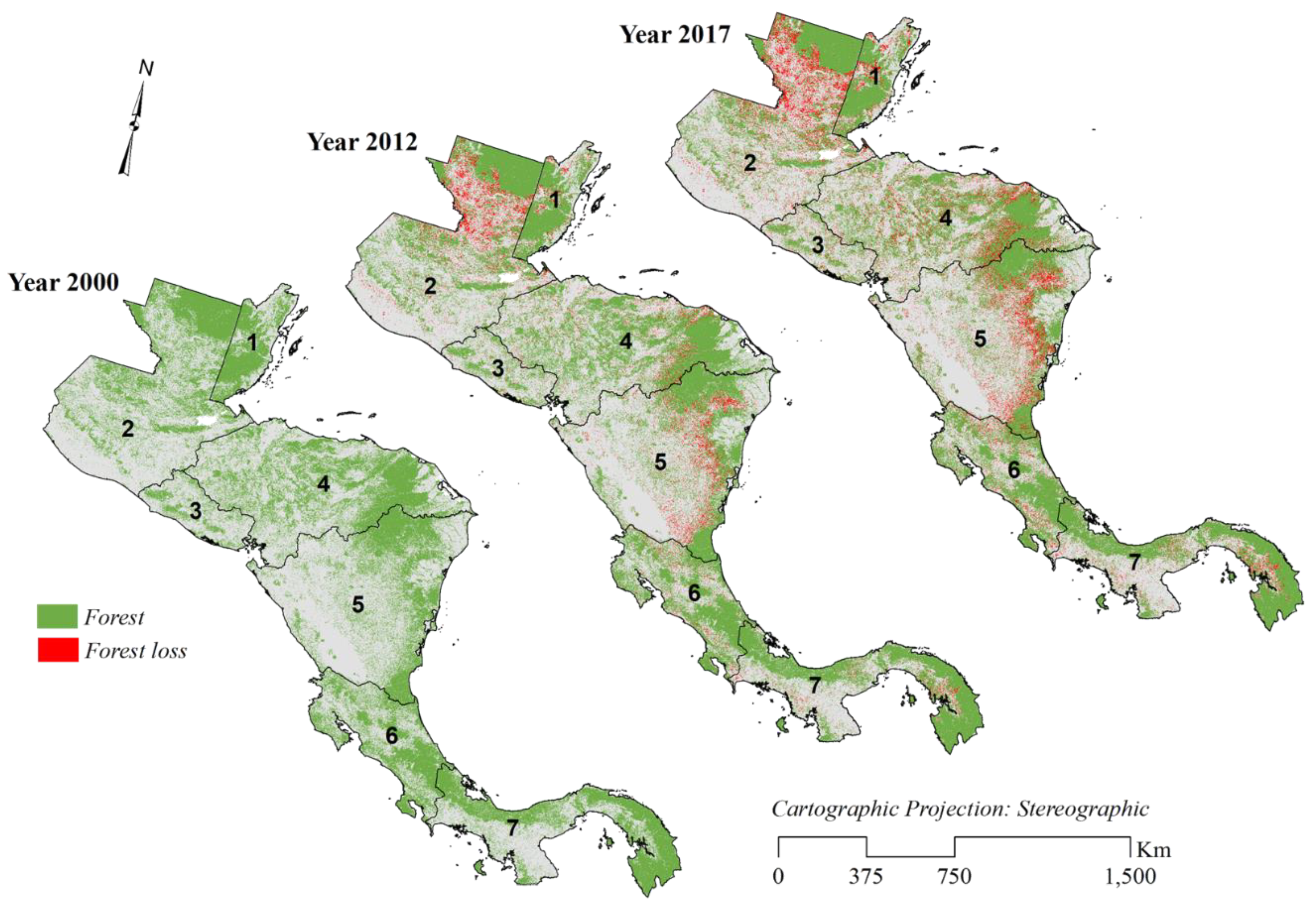
According to the results obtained, in 2000, Central America was covered by 43.8% of forest, a percentage that fell to 41.5% in 2012 and 38.3% in 2017 (Figure 5). In general, all countries presented a lower percentage of forest in the year 2017 compared to 2000. However, in the period 2000–2012 in El Salvador and Costa Rica, gain trends were observed (

Table 9. Forest area and percentage (regarding the national area) for the years 2000, 2012, and 2017.

Country	2000		2012		2017
	ha	%	ha	%	ha	%
Belize	1,417,703	62.5	1,344,840	59.3	1,269,564	56.0
Guatemala	4,241,251	38.4	3,657,041	33.1	3,306,148	29.9
El Salvador	647,669	30.8	682,058	32.4	629,858	30.0
Honduras	5,002,575	44.1	4,919,343	43.3	4,412,016	38.9
Nicaragua	4,532,602	34.8	4,071,153	31.2	3,667,438	28.1
Costa Rica	2,814,824	55.6	2,824,883	55.8	2,694,207	53.2
Panamá	4,225,595	57.1	4,171,767	56.3	4,030,640	54.4
Central America	22,882,219	43.8	21,671,085	41.5	20,009,871	38.3

).

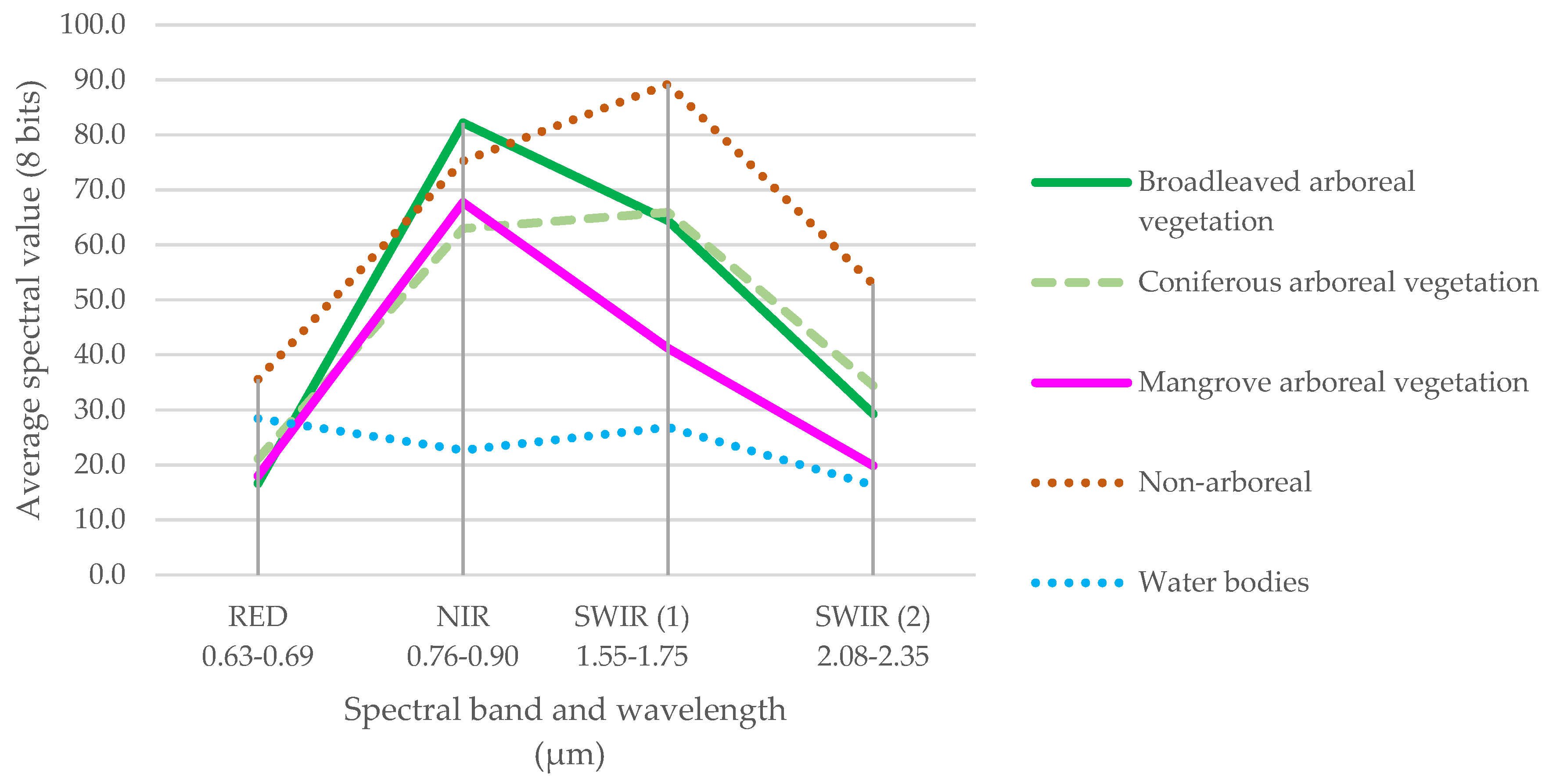
In terms of forest types of the total forest area of Central America, in 2017, 92.4% corresponded to broadleaf forest, 5.7% to coniferous forest, and 1.9% to mangrove forest. In the years 2000, 2012, and 2017, the area of broadleaf forest in Central America corresponded to 21,244,989 ha; 19,914,860 ha, and 18,489,948 ha; that of coniferous forest at 1,257,003 ha, 1,362,352 ha, and 1,137,548 ha, and that of mangrove forest at 380,228 ha, 393,873 ha, and 382,374 ha.

3.3. Forest Cover Change Dynamics

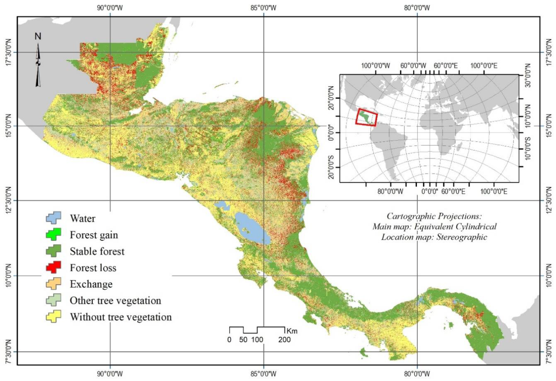
In addition to individually evaluating the forest area in each year, a forest cover change dynamics multitemporal analysis was performed. The change categories refer specifically to gains and losses that, from the forest monitoring perspective, correspond to deforestation and forest regeneration. Persistence refers to the absence of such changes, areas that in this study are within the categories of stable forest; other tree vegetation; exchange; without tree vegetation, and water. 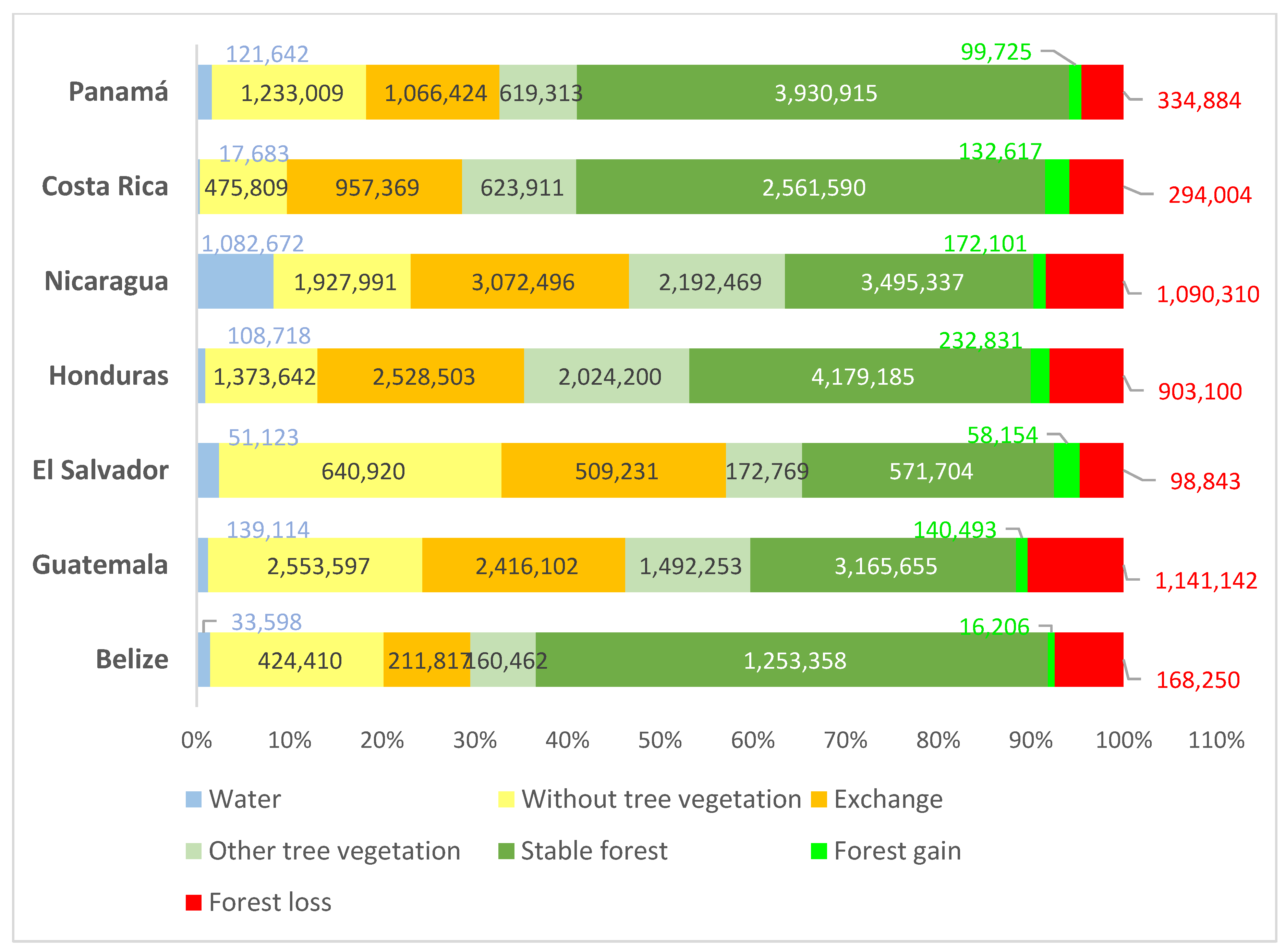Figure 6 shows the Central America forest cover change dynamics map for the period 2000–2017, and the percentage distribution of stable forest with respect to the rest of the categories of forest cover change dynamics in relation to the total area of each country is shown in Figure 7.

The highest proportions of stable forest were found in Belize, Panama, and Costa Rica, and the lowest in Nicaragua, Guatemala, and El Salvador. Regarding the exchange (associated with migratory agriculture processes), the greatest extensions (ha) were found in Nicaragua, Honduras, and Guatemala, countries that at the same time presented the greatest areas of forest loss. Regarding the areas without tree vegetation (associated with agricultural crop areas, urban areas, and other areas without tree vegetation), the highest proportion was found in El Salvador. In the category of other tree vegetation (mainly early secondary vegetation), the highest percentages with respect to the other categories, and also in terms of area, were found in Nicaragua and Honduras. In proportional terms, it was in Costa Rica and El Salvador where the highest gains were located.

For Central America as a whole, the average deforestation in the first period was 197,443 ha/year (2000–2012), and that of the second period was 332,243 ha/year (2012–2017). The average for the entire period was 264,843 ha/year (2000–2017). The first monitoring event in 2018 showed deforestation of 167,976 ha for that year, which is below the averages of both periods but very close to that of the first period.

Table 10. Average annual deforestation in Central American countries for the periods 2000–2012, 2012–2017, 2000–2017, and for the year 2018.

Country	Deforestation by Period (ha/Year)			Deforestation 2018 (ha)
	2000–2012	2012–2017	2000–2017
Belize	7748	15,055	11,402	7260
Guatemala	65,854	70,179	68,016	29,583
El Salvador	3887	10,440	7163	2161
Honduras	32,981	101,465	67,223	50,339
Nicaragua	57,216	80,743	68,980	53,494
Costa Rica	13,611	26,135	19,873	6702
Panamá	16,146	28,226	22,186	18,436
Central America	197,443	332,243	264,843	167,976

shows a summary of the annual deforested area by country in the periods 2000–2012, 2012–2017, 2000–2017, and that of the year 2018.

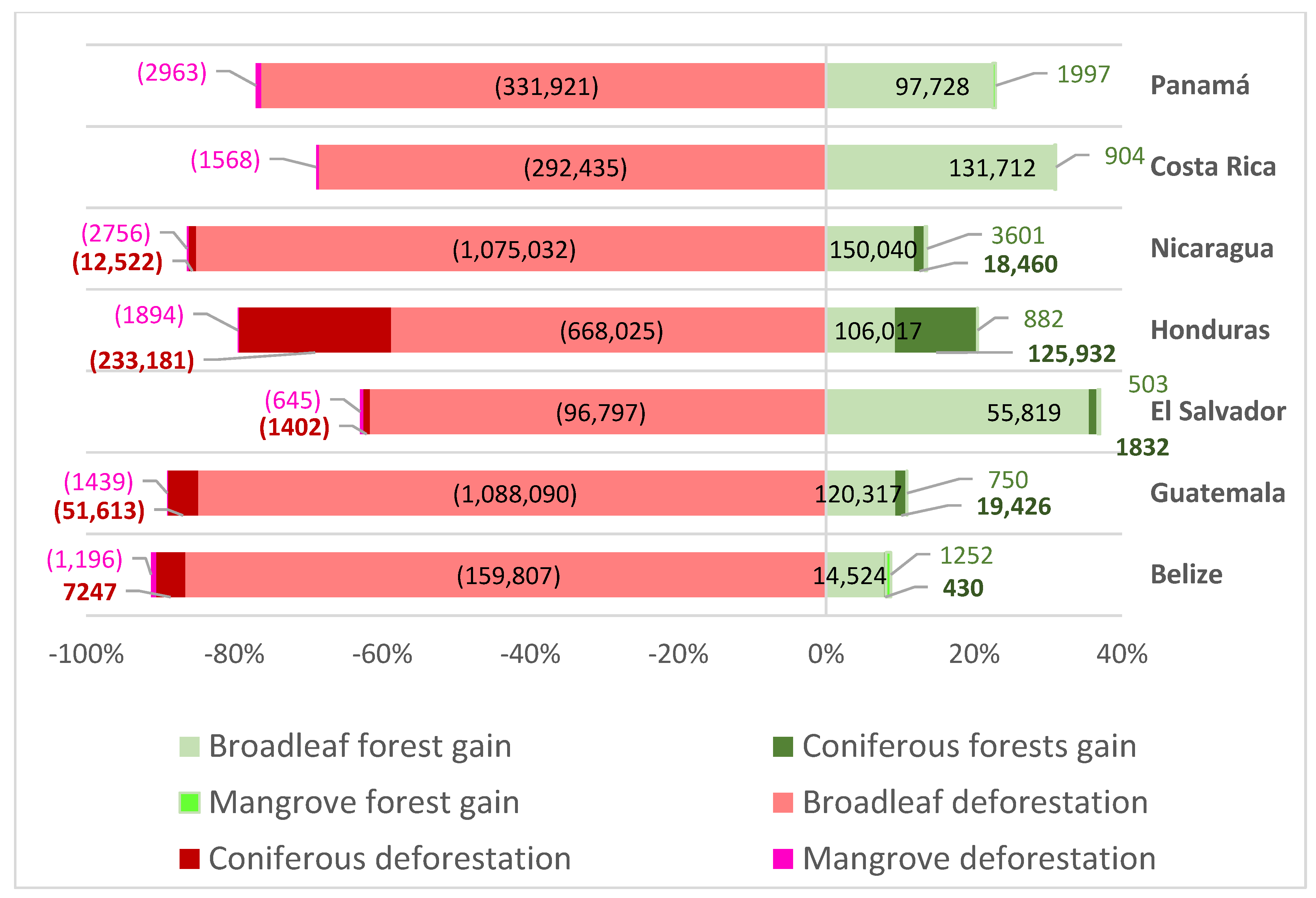
By forest type, in the 2000–2012 period, the annual loss of broadleaved forest in Central America was 190,600 ha/year, and it went up to 284,982 ha/year in the 2012–2017 period. The coniferous forest presented an average annual loss of 6763 ha/year in the first period, and it went up to 44,961 ha/year in the second. The largest increase in annual average deforestation by forest type occurred in the coniferous forest of Honduras, which went from 3778 ha/year in the first period to 37,570 ha/year in the second. A percentage of 29.3 of the total deforestation in Central America of the broadleaf forest occurred in Guatemala, 29.0% in Nicaragua, and 18% in Honduras. As for the coniferous forest, 76.2% of the losses were in Honduras and 16.9% in Guatemala. Panama concentrated 23.8% of the region’s losses in the mangrove forest, Nicaragua 22.1%, Honduras 15.2%, Costa Rica 12.6%, Guatemala 11.5%, Belize 9.6%, and El Salvador 5.2%.

Total gains for the region in the 2000–2012 period were 1,158,185 ha of which 26% were deforested in the following period, which means that of these gains only 852,126 ha remained in 2017. For the period 2012–2017, as it is a relatively short time to assess forest regeneration, gains were not analyzed. For the 2000–2017 period, 79.3% of the total forest gains in the region occurred in broadleaf forest, 19.5% in conifers, and 1.2% in mangrove. 22.2% of the gains in the broadleaf forest were in Nicaragua, 19.5% in Costa Rica, 17.8% in Guatemala, 15.7% in Honduras, and 14.5% in Panama. In the coniferous forest 75.8% of the gains were in Honduras, 11.7% in Guatemala, and 11.1% in Nicaragua. In relation to the mangrove gains, 36.4% of the total of the region occurred in Nicaragua, 20.2% in Panama, and 12.7% in Belize (Figure 8).

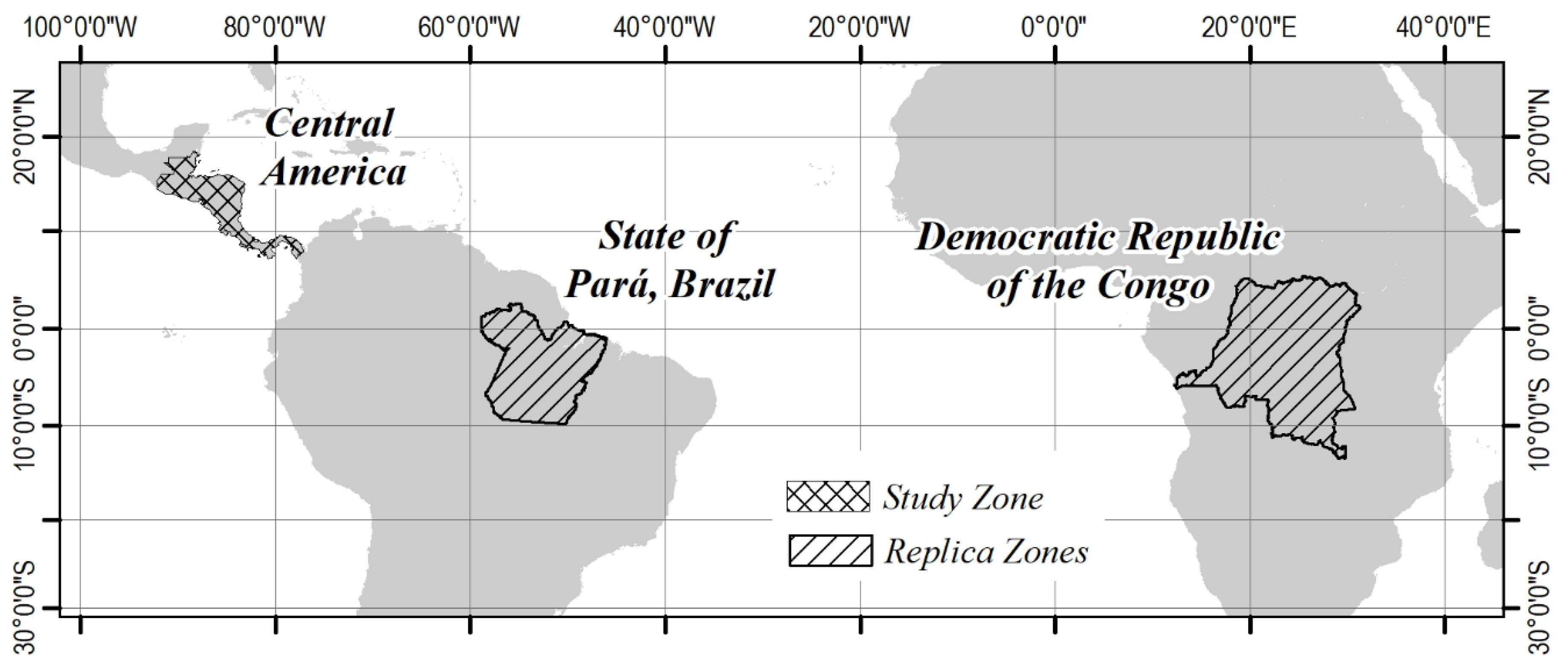
3.4. Application of the Methodology in Other Tropical Zones

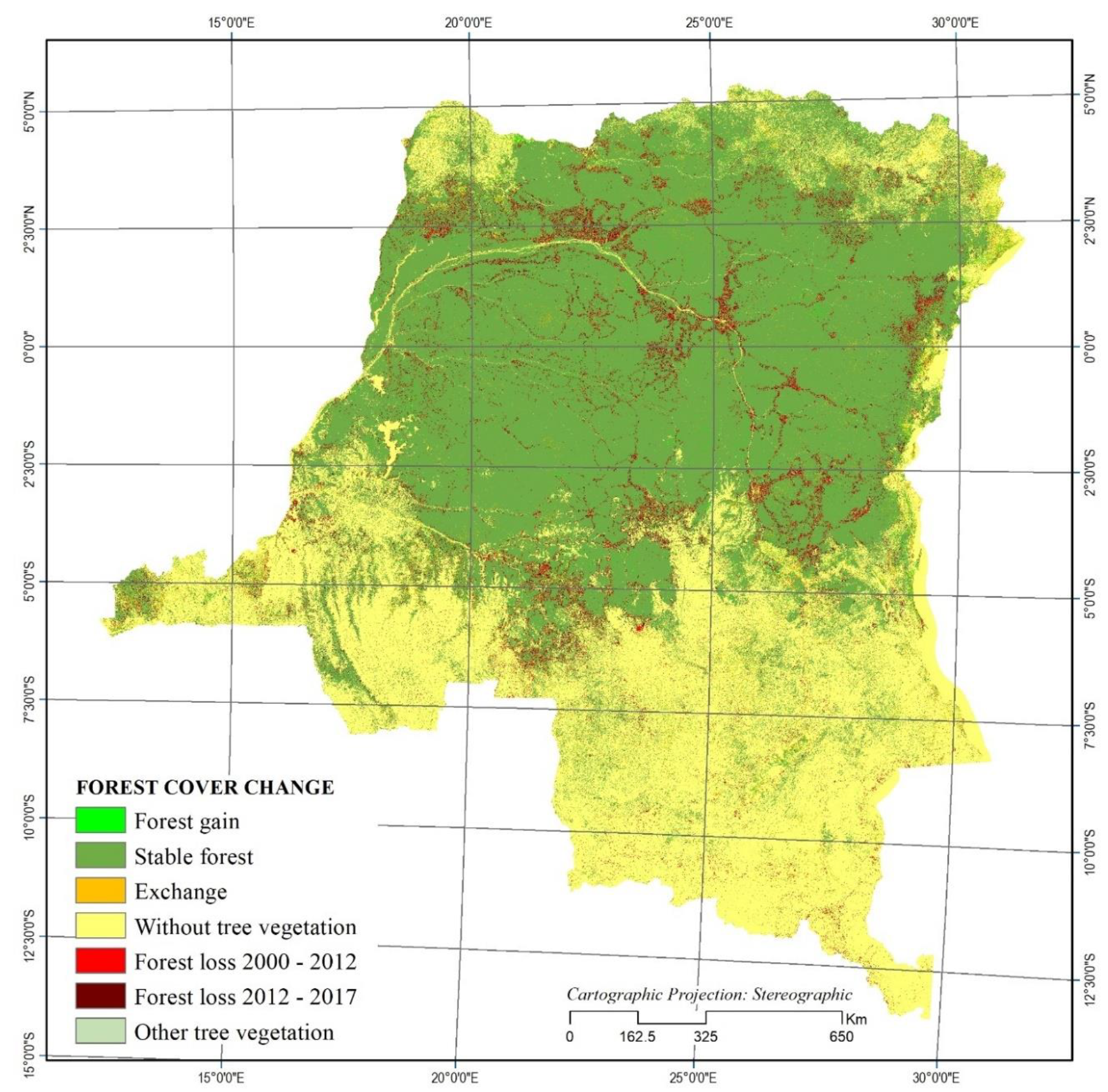
The results of replicating the methodology in the Democratic Republic of the Congo (DRC) showed that forest area decreased from 59% in 2000 to 52.2% in 2017 (

Table 11. Forest area for the years 2000, 2012, and 2017 in the Democratic Republic of the Congo (DRC).

	2000	2012	2017
Forest area (ha)	138,161,799	134,401,097	129,351,418
% of the national territory	59	57.4	52.2

).

The total forest loss in the country in the 2000–2017 period was 11,163,201 ha of which 6,113,521 ha were deforested in the 2000–2012 period and 5,049,679 ha in the 2012–2017 period (

Table 12. Forest change dynamics 2000–2017 in the Democratic Republic of the Congo (DRC).

Forest Change 2000–2017	Ha	%
Stable forest	126,998,598	54.22
Without tree vegetation	88,430,193	37.76
Exchange areas	5,228,664	2.23
Other tree vegetation	33,781	0.01
Forest gain	2,352,820	1.00
Forest loss	11,163,201	4.77
Total	234,207,257	100

).

Figure 9 shows the forest dynamics map of the Democratic Republic of the Congo (DRC), obtained as part of the replication of the methodology developed in this study.

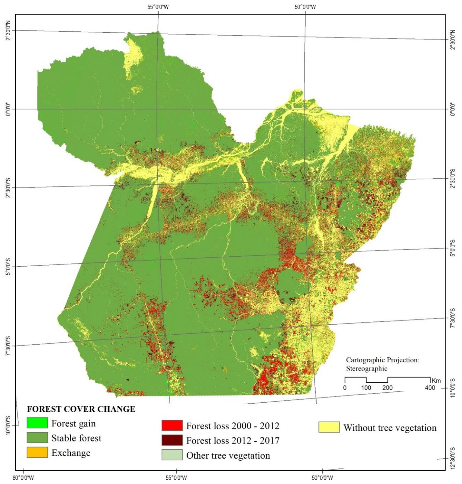
In the State of Pará, Brazil, the results show that forest area decreased from 81.3% in 2000 to 75.3% in 2017 (

Table 13. Forest area for the years 2000, 2012, and 2017 in the State of Pará, Brazil.

	2000	2012	2017
Forest area (ha)	101,869,009	98,021,479	94,344,978
% of the national territory	81.3	78.2	75.3

).

The total loss of State forest in the 2000–2017 period was 9,378,400 ha of which 5,701,899 ha were deforested in the 2000–2012 period and 3,676,501 ha in the 2012–2017 period (

Table 14. Forest change dynamics 2000–2017 in the State of Pará, Brazil.

Forest Change 2000–2017	Ha	%
Stable forest	92,490,608	73.78
Without tree vegetation	16,323,787	13.02
Exchange areas	5,308,008	4.23
Other tree vegetation	12,162	0.01
Forest gain	1,854,369	1.48
Forest loss	9,378,400	7.48
Total	125,367,334	100

).

Figure 10 shows the forest dynamics map of the State of Pará, Brazil, obtained as part of the replication of the methodology developed in this study.

4. Discussion

Most official forest cover maps prepared to date in Central America were generated independently by each country [6,7,8,9,10,11,12,13,14,15,16], making it difficult to integrate to obtain an overview of the situation and evolution of forests in the regional context. In response to this, in this research a methodological framework was developed to generate cost-efficient national maps of forest cover in Central America as a whole. The similarities of tropical countries in terms of vegetation types facilitated the generation of these maps by using satellite data, multisource secondary data, and training samples on a shared basis. The applied regional approach offers advantages in terms of reducing costs and time, as well as improving the consistency and coherence of reports at different territorial levels (regional and national), reducing duplication of efforts, and optimizing these forms of technical and financial resources.

The results indicate that in Central America, all the countries presented a lower percentage of forest in 2017 compared to 2000. This general trend of decrease at the regional level is consistent with that observed for the period 2000–2010 in the regional study by CATHALAC [4].

The trends of decrease in forest cover observed in this research would also be in line with the official data reported to FRA-2015 by most of the countries in the region [29], with the exception of Costa Rica, where the data indicated a trend towards a constant increase in forest cover since 1990 that had continued until 2015 [30], and in El Salvador, which according to data reported in FRA-2015, had a constant trend towards a forest cover decrease in the period 1990–2015 [31]. However, in this study, in the period 2000–2012, increases in forest cover of 1.6% and 0.2%, respectively, were observed in both countries, and a trend of decrease in the following period, 2012–2017, in both.

At this point, it should be taken into account that, for example, in El Salvador in the report to the FRA-2015, since there were no historical data about forest cover loss, an annual rate of deforestation was estimated using expert’s criteria, applying it to the 2002 map, and projecting the previous and subsequent years [31]. In contrast, the global land cover data generated by European Space Agency (ESA) [32] for El Salvador shows a trend of recovery of the country’s forest cover from 1992 to 2000, and from this year, it seeks to stabilize. However, it should be taken into account that, compared to the 30 m resolution and 30% canopy threshold used in this study, the ESA data were generated at 300 m resolution and considering a canopy greater than 15% to classify a pixel as forest, resulting in a larger area of forest detected. Many pixels included in this research within the category other tree vegetation (non-forest) would be considered forest in the data provided by ESA.

In Costa Rica, the forest gain trend from 1990 that continued in 2015, which was reported to FRA-2015, does not coincide with what was observed in this research, which showed a forest cover decrease in the period 2012–2017. In this country in the FRA-2015 report, forest cover for 2010 was estimated by applying a linear extrapolation based on data from 2000 and 2005; to obtain the cover forest area of the year 2015, the area of the 2013 map was projected, using the trend 2005–2010 [30]. The losses that could occur in the period 2012–2017 in Costa Rica observed in this study were not included in the projection to 2015 of the report to the FRA, which assumed the continuity of a gain trend, which could contribute to the differences between both sources.

In Honduras, the loss of forest cover reported at the REDD+ reference level for the 2000–2016 period was 22,696 ha/year [17], much less than the 67,223 ha/year obtained for the 2000–2017 period in this study, and even lower than the average forest loss rate obtained for the 2000–2012 period of 32,981 ha/year and 101,465 ha/year for the 2012–2017 period. These differences could be due to the fact that, by national definition, forest losses within areas included in the category of Sustainable Forest Management and forest cover losses caused by the pine beetle pest that affected the country in 2015–2017, were excluded in the official quantification of deforestation, but both cases were considered in this investigation. Official figures from August 2016 indicated that this pest had already affected 495,967 hectares of the country’s coniferous forest [17].

The last official report on forest cover in Guatemala indicated that the country had maintained 33% of its forest by 2016 [15], a value higher than that observed in this study of 30% by 2017, but similar to the case of 2012 where 33.9% was officially reported, and 33.1% was obtained in this investigation.

The percentage of Panama forest cover officially presented in 2019 was higher than those obtained in this study; compared to percentages of 72.8%, 66.1%, and 65.4% of coverage of ‘forests and other forest land’, respectively, for 2000, 2012, and 2019 [16], in this research values of 57.1%, 56.3%, and 54.4% were obtained for the years 2000, 2012, and 2017, respectively. The differences could be influenced by the category stubble and shrubs vegetation that was included within forest cover in the 2019 study, which was considered an initial vegetation state in transition to forest.

In Nicaragua, the REDD+ reference level values indicate that for the years 2000, 2010, and 2015 the percentages of forest cover in the country were 41.8%, 31.06%, and 30.21%, respectively [14]. The data obtained in this study was lower, 34.38% for the year 2000, 31.2% for 2012, and 28.1% for 2017, but in both sources, a trend towards the decrease in the forest cover is marked, which places Nicaragua, along with Guatemala and Honduras, as countries with the largest deforested areas in the period analyzed in Central America.

In Belize, the information generated by Cherrington et al. [8,18], based on Landsat images, for the year 2000 reported a forest cover of 65.8% and 61.6% for 2012; in this study, for those same years, 62.5% and 56.0% were obtained. Part of these differences could be related to the fact that the model developed and applied in this research has not been able to adequately detect the coniferous forest areas in the center of the country. The reason for the limitation in the detection of this type of forest could be due to the fact that the coniferous forests of Central America present a high variability in the density of the tree canopy, presenting large extensions of sparse forests that are spectrally confused with dry scrubs.

Scrubs and dry forests also mix spectrally with crop areas, mainly because this type of vegetation loses its canopy at the period of least rainfall of the year. These detection limitations could at the same time be the reason that the lowest accuracies in the forest mapping generated in this study occurred in Honduras, the country with the highest proportion of coniferous forest in the region, and in El Salvador, which has the highest proportion of dry forest in the region with respect to the total area of national forest cover.

In general, for Central America the percentage of forest cover obtained in this study with respect to the data in the FRA-2015 [29] report is less than 1% in 2000 and 2017 and higher by 1% in 2012. In the Democratic Republic of the Congo, with respect to the official data presented to the UNFCCC [33], the percentage of forest cover of the year 2000 obtained in this study is higher by 2% but similar in 2012 when compared to the 2014 data reported to the UNFCCC (0.1% difference). In the case of the State of Pará, Brazil, when compared to the data generated by the MapBiomas Project [34], the percentage of forest cover obtained in this study is less by 1.3% in 2012 and is also less for 2000 and 2017 with a difference of 3.3% and 3.9%, respectively.

Potential improvements in this study are expected in the future, incorporating independent validation processes of the secondary data sources used (such as the national forest masks and secondary data of tree cover loss), as well as the use of higher resolution satellite images, such as Sentinel and digital terrain elevation models. These potential improvements are based on the findings of recent studies where it has been found that the combination of multisource data, which were not used in this study, could provide significant improvements in the detection of forest types, as in the case of Sentinel-2A (S2), Sentinel-1A (S1) in dual polarization, and Shuttle Radar Topographic Mission Digital Elevation (DEM) combined with multitemporal Landsat images [35]. Other improvements would be related to the inclusion of secondary data sources to exclude from forest losses the areas that, being subject to forest management, cause temporary reductions in the tree canopy and other forest losses that are legally authorized.

5. Conclusions

With this research, a theoretical–methodological framework has been developed and applied to cost-efficiently prepare national cartography on forest cover, temporarily consistent, and scalable at the supranational level in the Central American region and in other tropical regions of the world. Forest maps were generated considering the Central American region as a whole, with the expectation that later the regional classification will be adopted to the country level for multitemporal forest cover changes study. With the proposed methodological development, progress has been made with respect to the previous studies carried out in Central America, going from classifying individual scenes of Landsat satellite images and separately by country to doing so in a regional context. Additionally, new geoprocessing elements have been incorporated into the digital classification procedures for satellite images, such as the automated extraction of training samples from secondary sources, the use of official national reference maps that respond to nationally adopted forest definitions, and automation of post-classification adjustments incorporating expert criteria. The time involved in the classification process using automated workflows through the implemented algorithms was significantly reduced in relation to the traditional classification methods used in the countries of the region.

In terms of forest loss area by country, the largest deforested areas in the period 2000–2017 were in Guatemala, Nicaragua, and Honduras, countries where the greatest areas of gain were also located. However, when calculating the percentage of gain with respect to the total area of each country, the highest proportions were observed in El Salvador and Costa Rica. In terms of the percentage of forest with respect to the total national territory, Belize is the country that maintains the highest forest cover in the region, followed by Panama and Costa Rica; the lowest percentage of national forest was observed in Honduras, Nicaragua, Guatemala, and El Salvador. In terms of accuracy of the classifications obtained for the forest/non-forest maps, the lowest was obtained in Honduras, Guatemala, El Salvador, and Nicaragua, corresponding on the scale of the Kappa index to the category of moderate concordance. The best accuracies were obtained in Belize, Panama, and Costa Rica, ranking according to the Kappa index in the category of considerable agreement.

The application of the classification model generated in this study to other tropical areas of great territorial extension, such as the Democratic Republic of the Congo (DRC) and the State of Pará in Brazil, allows us to conclude that with the applied method, in addition to reducing the time involved in the analysis of forest cover dynamics in territories of large areas such as those selected, it is also possible to improve the scale of the existing mappings. As was the case in the DRC, where the best map obtained as input was 300 m of resolution in 2012, applying the model resulted in a 30 m map. Although, due to limitations of the research resources a validation of the results was not carried out, when comparing the results obtained with the official data of the country presented to the UNFCCC in terms of percentage of coverage at the national level, in 2012 a difference of 0.1% was found compared to the results of this study.

References

1. Muchoney, D.; Borak, J.; Chi, H.; Friedl, M.; Gopal, S.; Hodges, J.; Morrow, N.; Strahler, A. Application of the MODIS global supervised classification model to vegetation and land cover mapping of Central America. Int. J. Remote Sens. 2000, 21, 1115–1138. [Google Scholar] [CrossRef]
2. Vreugdenhil, D.; Meerman, J.; Meyrat, A.; Gómez, L.D.; Graham, D.J. Map of the Ecosystems of Central America: Final Report; World Bank: Washington, DC, USA, 2002. [Google Scholar]
3. Giri, C.; Jenkins, C. Land cover mapping of Greater Mesoamerica using MODIS data. Can. J. Remote Sens. 2005, 31, 274–282. [Google Scholar] [CrossRef]
4. CATHALAC-SIMEPAR. Mapa Centroamericano de Cobertura y Uso de la Tierra: Cambios de Cobertura y Uso de la Tierra 1980-1990-2000-2010; Technical Report; PREVDA: Panama City, Panama, 2011. [Google Scholar]
5. Bardales, D. Mapa Forestal de Honduras 1995; AFE-COHDEFOR: Tegucigalpa, Honduras, 1998. [Google Scholar]
6. Castellanos, E.; Regalado, O.; Pérez, G.; Montenegro, R.; Ramos, V.H.; Incer, D. Mapa de Cobertura Forestal de Guatemala 2006 y Dinámica de la Cobertura Forestal 2001–2006; Technical Report; Universidad de Valle de Guatemala: Guatemala City, Guatemala; Instituto Nacional de Bosques: Guatemala City, Guatemala; Consejo Nacional de Áreas Protegidas: Guatemala City, Guatemala; Universidad Rafael Landívar: Guatemala City, Guatemala, 2011. [Google Scholar]
7. Regalado, O.; Villagrán, X.; Pérez, G.; Castellanos, E.; Martínez, G.; Incer, D.; Ramos, V.H.; Molina, O.; Beltetón, C.; Gómez, J.M. Mapa de Cobertura Forestal de Guatemala 2010 y Dinámica de la Cobertura Forestal 2006–2010; National Forestry Institute (INAB): Guatemala City, Guatemala; National Council for Protected Areas (CONAP): Guatemala City, Guatemala; Universidad del Valle de Guatemala: Guatemala City, Guatemala; Universidad Rafael Landívar: Guatemala City, Guatemala, 2012. [Google Scholar]
8. Cherrington, E.A.; Ek, E.; CHO, P.; Howell, B.F.; Hernandez, B.E.; Anderson, E.R.; Flores, A.I.; Garcia, B.C.; Sempris, E.; Irwin, D.E. Forest Cover and Deforestation in Belize: 1980–2010; SERVIR-Cathalac: Panama City, Panama, 2010. [Google Scholar]
9. Sierra, R.; Cambronero, A.; Vega, E. Patrones y Factores de Cambio de la Cobertura Forestal Natural de Costa Rica, 1987–2013; Gobierno de Costa Rica/Fondo Cooperativo para el Carbono de los Bosques (FCPF): San José, Costa Rica, 2015.
10. Duarte, E.; Orellana, O.; Maradiaga, I.; Casco, F.; Fuentes, D.; Jimenez, A.; Emanuelli, P.; Milla, F. Mapa Forestal y de Cobertura de la Tierra de Honduras: Análisis de Cifras Nacionales; Programa REDD-CCAD/GIZ; ICF: Tegucigalpa, Honduras, 2014. [Google Scholar]
11. Ortiz Malavassi, E. Cartografía Base Para el Inventario Forestal Nacional de Costa Rica 2013-2014; SINAC, Programa REDD-CCAD/GIZ; FONAFIFO: San José, Costa Rica, 2015.
12. Catalán, M.; Castillo, F. Mapa de Cobertura Forestal por Tipo y Subtipo de Bosque para la República de Guatemala, 2012; INAB-CONAP: Guatemala City, Guatemala, 2015. [Google Scholar]
13. Castillo, M.; Samaniego, R.; Kindgard, A. Mapa de cobertura y uso de la tierra 2012; ONU-REDD (FAO); Ministerio de Ambiente de Panamá: Panama City, Panama, Programa, 2015. [Google Scholar]
14. MARENA. Niveles de Referencia de las Emisones Forestales República de Nicaragua; Ministerio del Ambiente y los Recursos Naturales: Managua, Nicargua, 2019; p. 56.
15. Grupo Interinstitucional de Monitoreo de Bosques y Uso de la Tierra (GIMBUT). Mapa de Cobertura Forestal de Guatemala 2016 y Dinámica de la Cobertura Forestal 2010–2016; Technical Report; Instituto Nacional de Bosques: Guatemala City, Guatemala; Consejo Nacional de Áreas Protegidas: Guatemala City, Guatemala; Ministerio de Agricultura, Ganadería y Alimentación: Guatemala City, Guatemala; Ministerio de Ambiente y Recursos Naturales: Guatemala City, Guatemala; Universidad de Valle de Guatemala: Guatemala City, Guatemala; Universidad Rafael Landívar: Guatemala City, Guatemala, 2019; Volume 127. [Google Scholar]
16. MiAmbiente. Diagnóstico sobre la Cobertura de Bosques y otras Tierras Boscosas de Panamá, 2019; Ministerio de Ambiente: Panama City, Panama, 2020.
17. ICF; MiAmbiente+. Propuesta Nivel de Referencia Forestal de Honduras; ONU-REDD/FAO: Roma, Italia, 2020. [Google Scholar]
18. Cherrington, E.; Cho, P.; Waight, I.; Escalante, A.; Nabet, J.; Usher, L.; Santos, T. Belize Forest Cover Change, 2010–2012: Summary of Findings. Ministry of Forestry, Fisheries, and Sustainable Development of Belize (MFFSD); UB-ERI.: Belmopan, Belize; Lancaster University: Lancaster, UK; CATHALAC: Panamá, Panama, 2012. [Google Scholar]
19. Gutman, G.; Huang, C.; Chander, G.; Noojipady, P.; Masek, J.G. Assessment of the NASA–USGS global land survey (GLS) datasets. Remote Sens. Environ. 2013, 134, 249–265. [Google Scholar] [CrossRef]
20. Wulder, M.A.; White, J.C.; Loveland, T.R.; Woodcock, C.E.; Belward, A.S.; Cohen, W.B.; Fosnight, E.A.; Shaw, J.; Masek, J.G.; Roy, D.P. The global Landsat archive: Status, consolidation, and direction. Remote Sens. Environ. 2016, 185, 271–283. [Google Scholar] [CrossRef] [Green Version]
21. Moore, R.T.; Hansen, M.C. Google Earth Engine: A New Cloud-Computing Platform for Global-Scale Earth Observation Data and Analysis; American Geophysical Union: Washington, DC, USA, 2011; Volume 1, p. 2. [Google Scholar]
22. Gorelick, N. Google Earth Engine. In Proceedings of the European Geosciences Union (EGU) General Assembly Conference, Vienna, Austria, 7–12 April 2013; Volume 15, p. 11997. [Google Scholar]
23. Hansen, M.C.; Loveland, T.R. A review of large area monitoring of land cover change using Landsat data. Remote Sens. Environ. 2012, 122, 66–74. [Google Scholar] [CrossRef]
24. Hansen, M.C.; Potapov, P.V.; Moore, R.; Hancher, M.; Turubanova, S.A.; Tyukavina, A.; Thau, D.; Stehman, S.V.; Goetz, S.J.; Loveland, T.R. High-resolution global maps of 21st-century forest cover change. Science 2013, 342, 850–853. [Google Scholar] [CrossRef] [PubMed] [Green Version]
25. Olson, D.M.; Dinerstein, E.; Wikramanayake, E.D.; Burgess, N.D.; Powell, G.V.; Underwood, E.C.; D’amico, J.A.; Itoua, I.; Strand, H.E.; Morrison, J.C. Terrestrial Ecoregions of the World: A New Map of Life on Earth: A new global map of terrestrial ecoregions provides an innovative tool for conserving biodiversity. Bioscience 2001, 51, 933–938. [Google Scholar] [CrossRef]
26. Strahler, A.H. The use of prior probabilities in maximum likelihood classification of remotely sensed data. Remote Sens. Environ. 1980, 10, 135–163. [Google Scholar] [CrossRef]
27. Foody, G.M.; Campbell, N.A.; Trodd, N.M.; Wood, T.F. Derivation and applications of probabilistic measures of class membership from the maximum-likelihood classification. Photogramm. Eng. Remote Sens. 1992, 58, 1335–1341. [Google Scholar]
28. Landis, J.R.; Koch, G.G. The measurement of observer agreement for categorical data. Biometrics 1977, 33, 159–174. [Google Scholar] [CrossRef] [PubMed] [Green Version]
29. FAO. Evaluación de Los Recursos Forestales Mundiales 2015: Como Están Cambiando Los Bosques del Mundo? Segunda Edición; FAO: Roma, Italia, 2016. [Google Scholar]
30. Chavarría Espinoza, I. Evaluación de los Recursos Forestales Mundiales 2015: Informe Nacional Costa Rica; SINAC-MINAE: San José, Costa Rica, 2014.
31. Herrera Guzmán, R.A.; Cruz Rodríguez, E.A. Evaluación de los Recursos Forestales Mundiales 2015: Informe Nacional El Salvador; DGFCR-MAG: San Salvador, El Salvador, 2014. [Google Scholar]
32. ESA Land Cover CCI. Product User Guide, version 2.0; ESA: Paris, France, 2017. [Google Scholar]
33. MEDD. Niveau D’Emissions de Reference des Forets Pour la Reduction des Emissions Dues a la Deforestation en République Démocratique du Congo; Ministère de l’environnement et de Développement Durable: Kinshasa, République Démocratique du Congo, 2018.
34. MapBiomas. Project MapBiomas. Available online: www.mapbiomas.org (accessed on 8 September 2019).
35. Liu, Y.; Gong, W.; Hu, X.; Gong, J. Forest Type Identification with Random Forest Using Sentinel-1A, Sentinel-2A, Multi-Temporal Landsat-8 and DEM Data. Remote Sens. 2018, 10, 946. [Google Scholar] [CrossRef] [Green Version]
Figure 1. Example of a mosaic of Landsat satellite images of Central America.
Remotesensing 12 02705 g001
Figure 2. Phases and methodological steps applied.
Remotesensing 12 02705 g002
Figure 3. Average spectral signatures of different vegetation types from Central America derived from Landsat ETM+ images.
Remotesensing 12 02705 g003
Figure 4. Zones selected for scaling up and replication of the methodology.
Remotesensing 12 02705 g004
Figure 5. Forest cover maps generated in this study in the Central America region for the years 2000, 2012, and 2017. 1 = Belize, 2 = Guatemala, 3 = El Salvador, 4 = Honduras, 5 = Nicaragua, 6 = Costa Rica, and 7 = Panama.
Remotesensing 12 02705 g005
Figure 6. Central America forest cover change dynamics. Period 2000–2017.
Remotesensing 12 02705 g006
Figure 7. Percentage distribution and area of the forest cover change dynamics categories in Central American countries.
Remotesensing 12 02705 g007
Figure 8. Forest cover loss/gain ratio by country in the period 2000–2017.
Remotesensing 12 02705 g008
Figure 9. The Democratic Republic of the Congo forest cover change dynamics. Period 2000–2017.
Remotesensing 12 02705 g009
Figure 10. The State of Pará, Brazil, forest cover change dynamics. Period 2000–2017.
Remotesensing 12 02705 g010