Article

Evaluating a Suitable Aquaculture Site Selection Model for Cobia (Rachycentron canadum) during Extreme Events in the Inner Bay of the Penghu Islands, Taiwan

1
Department of Environmental Biology and Fisheries Science, National Taiwan Ocean University, Keelung 20224, Taiwan
2
Center of Excellence for Oceans, National Taiwan Ocean University, Keelung 20224, Taiwan
3
Penghu Marine Biology Research Center, Fisheries Research Institute, Council of Agriculture, Executive Yuan, Penghu 88049, Taiwan
4
National Applied Research Laboratories, Taiwan Ocean Research Institute, Taipei 10622, Taiwan
*
Author to whom correspondence should be addressed.
Remote Sens. 2020, 12(17), 2689; https://doi.org/10.3390/rs12172689
Submission received: 29 July 2020 / Accepted: 18 August 2020 / Published: 20 August 2020
(This article belongs to the Special Issue Remote Sensing for Fisheries and Aquaculture)

Abstract

:
Despite numerous studies on the effect of a cold weather disaster on fisheries in 2008, no operational systems have been developed to monitor the threat of such an event to mariculturists in the Penghu Islands (PHI) region of Taiwan. The present study employed a suitable aquaculture site selection map of the inner bay of the PHI to reduce aquaculture losses and mortality rates of cobia (Rachycentron canadum) during extreme events. Daily marine environmental data, including sea surface temperature (SST), chlorophyll-a concentration (chl-a), and wind speed in the winter, were collected. An extreme event was defined as a period of over 11 days in a month of strong winds (>6 m/s). Four parameters in the PHI inner bay, including SST, cold-water intrusion days, chl-a, and offshore distance to the PHI coastline, were used to evaluate suitable aquaculture sites for cobia culture. The results indicated that La Niña events could not be used as a factor to detect cold-water intrusion events and select suitable aquaculture sites in the PHI. The evaluated suitable aquaculture site selection map, obtained using an arithmetic mean model and a geometric mean model, revealed that the avoidance sites during extreme events were concentrated in the northern and northwestern PHI. Suitable areas were concentrated in the southeastern areas. We further suggested that commercial cobia aquaculture operations in the PHI inner bay could be moved to the suitable sites in southeastern PHI during extreme events.

Graphical Abstract

1. Introduction

Concerns regarding the effect of marine environments on coastal aquaculture zones have increased in recent decades [1]. Aquaculture plays an increasingly crucial role in maintaining a consistent supply of aquatic species for human consumption [2,3]. Global aquaculture production (included finfish and shellfish) supplied an estimated 80 million tons of fish in 2016 [4]. Aquaculture accounted for the production of 53% of the global fish products consumed in 2016. Climate change and variations in environmental conditions are poised to compound the existing pressures on fisheries and aquaculture and pose a threat to the livelihood and food security of millions of people [5].
The cobia, Rachycentron canadum, is a large, migratory, coastal pelagic fish of the monotypic family Rachycentridae that is distributed worldwide in tropical and subtropical seas, with the exception of the eastern Pacific [6,7]. The cobia is a fish species that lives in the temperate zone and grows rapidly, reaching 6–8 kg after a year, which is suitable for market use. Because all parts of the cobia are utilized, they have a high economic product value. These characteristics have made cobia a popular aquaculture species in the Penghu Islands (PHI) [8]. Following successful artificial propagation of cobia fingerlings in Taiwan in 1994, farmers began commercial cobia culture operations in the inner bay of Penghu (black mark in Figure 1b). The process of a phased culture mode consists of bloodstock management, mass larval production, and management of the nursery and growth phases [8,9,10,11,12]. Cobia culture developments and techniques have reached maturity in the PHI, but the industry is still subject to natural disasters. These disasters in the PHI, such as typhoon events in the summer and cold-water intrusions in the winter, are major factors affecting cobia culture development and lead to increased mortality rates and reduced annual outputs [8,13].
Cold currents from the north and warm currents from the south flow through the Taiwan Strait (TS), which contains complex topographic features. The principal shallow topographies are the Chang-Yuen Ridge, off the western coast of Taiwan, and the Taiwan Bank, in the southwest section of the TS (Figure 1a). In winter, the main China Coastal Current (CCC) on the western side of the TS moves southward along the Chinese coast (Figure 1a). The CCC is partially blocked around the Chang-Yuen Ridge and thus moves back northward at the expense of southward intrusion (gray arrows in Figure 1a). Furthermore, the Kuroshio Branch Current (KBC) from the Penghu Channel is blocked at the Chang-Yuen Ridge (black arrows in Figure 1a). A study has indicated that the warm tongue of the KBC could occasionally advance northward from the Penghu Channel [14]. However, unusual cold-water intrusion disaster events (e.g., those in 2008 and 2011) from the offshore branch of the CCC threaten local marine aquaculture and wild fish around the PHI [9,15].
The wind speed during El Niño–Southern Oscillation (ENSO) events has a larger effect than other meteorological factors on sea surface temperature (SST) variation in the TS [9]. Studies have indicated that the wind in the TS is stronger during La Niña winters than during normal winters [9,15]. Another study revealed that changes in water temperature during La Niña led to a higher intensity of variations in hydrographic features than those during El Niño [16,17]. The effects of La Niña winters on marine populations and fisheries in the TS are not adequately understood. The SST in the southern TS is higher than 20 °C during a normal winter, but temperatures decreased to 13 °C in the La Niña winter of 2008 [16]. Therefore, the cold disaster was not an isolated event but was related to a periodic global climate effect. Despite numerous studies performed using satellite-recorded data and numerical models on the effect of the cold disaster event in 2008 on fisheries, no operational system has been developed to identify or monitor threats to mariculturists working in the TS and PHI. Suitable aquaculture site selection models have been developed to describe the relationships between the production of aquatic species and environmental factors, and identify suitable sites [3,18,19,20].
Thus, the objective of this study was to develop a suitable aquaculture site selection model for cobia in the inner bay of the PHI to reduce aquaculture losses and mortality rates of cobia during extreme weather events. Therefore, we collected daily wind speed data that were measured directly by a local gauge station in the wintertime (2002–2015) and classified each month into one of three categories based on the number of days with wind speeds over 6 m/s. We also classified them according to the ENSO events, which followed the standard from previous studies (Figure 2). Furthermore, the marine environmental factors of SST and chlorophyll-a (chl-a), cold-water intrusion days (InDs), and distance to the coastline in the gridded areas were used to create variable influence scores and relative weighting by using partial least squares regression (PLSR) (Figure 2). Finally, the suitability values, evaluated using an arithmetic mean model and a geometric mean model, were used to select the suitable aquaculture sites for avoidance sites, tolerance sites, and suitable sites for the location of cobia cage culture in the PHI.

2. Data and Methods

2.1. SST and Wind Speed Data Collected and Definition of Extreme Event

2.1.1. SST and Wind Speed Data

Daily satellite-derived SST data were extracted from a daily Advanced Very High Resolution Radiometer (AVHRR) infrared satellite over a 13-year period (2002–2015) and from archives of the regional High-Resolution Picture Transmission data library at the National Taiwan Ocean University [20]. High-resolution (1.1 km) SST images were produced using the Multi-Channel SST algorithm [21,22]. To investigate the annual and interseasonal variations of wintertime SST in Penghu, the time series of daily SST was estimated. We calculated the mean SST of a cloud-free pixel for 49 gridded areas (2.5 km2) in the inner bay in the center of the PHI (119.45°E–119.625°E, 23.5°N–23.675°N, Figure 1b), in wintertime (January and February).
According to a study, the flow of the KBC through the Penghu Channel in winter was correlated with the changing winds around the PHI [23,24]. Therefore, we collected winter daily wind speed data (every January and February) from the gauge station in the PHI during 2002–2015 (Figure 1b, gold star). Studies have reported that strong winds with speeds of more than 6 m/s and persisting over long periods led to extremely low SST events in the PHI [9,16,24]. Therefore, the monthly cumulative duration of the strong wind (>6 m/s) in days was categorized into three groups. Category A represented a cumulative duration of 1 to 6 days/month, category B was 7 to 11 days/month, and category C was over 11 days/month. Category C was defined as an “extreme event” in the PHI.

2.1.2. El Niño–Southern Oscillation

The Oceanic Niño Index was used as the primary indicator to monitor El Niño and La Niña alternating phases; such monitoring was done to be able to evaluate the effect of the climate variability of ENSO events on SST variation. The 3-month running mean of SST anomalies (SSTAs) was estimated in the Niño 3.4 region (5°N–5°S, 120°E–170°W) based on data covering 2002–2015. Events were defined as five consecutive overlapping 3-month periods with a ≥ +0.5° anomaly for warm (El Niño) events or ≤−0.5° anomaly for cold (La Niña) events. The threshold was further categorized into weak (0.5–0.9 SSTA), moderate (1.0–1.4), strong (1.5–1.9), and very strong (≥2.0) events. Very strong El Niño events were recorded in 2015. Strong La Niña events were recorded in 2008 and 2011 [25].

2.2. Environmental and Geographic Parameters

2.2.1. SST Anomalies

The monthly SST anomalies ( SST A g ) were calculated in 49 gridded areas to understand the changes in SST under the three categories as follows:
SST ¯ gij = 1 y , m SS T dij 1 y , m dij
SST A g = SST ¯ ymd SST ¯ gij
where y, m, and d denote the year (2002–2015), month (January and February), and day, respectively, and g denotes the number of grids (1–49). The terms i and j represent longitude (119.45°E–119.625°E) and latitude (23.5°N–23.675°N), respectively.

2.2.2. Cobia’s Tolerance for SST and the Cold-Water Intrusion Days

Changes in water temperature influenced the growth, behavior, bait preference, and mortality of cobia [12,13,26]. The cobia growth rates were highest for SSTs of 22 °C–32 °C, and growth rates were reduced for SSTs below 20 °C [26]. Furthermore, when the SSTs were below 15 °C, cobia exhibited strange behaviors. They displayed abnormal swimming behaviors. SSTs below 14 °C led to high mortality rates [12,13]. Cobia’s SST toleration threshold was defined as 15 °C for aquaculture in the PHI. The number of days with an SST below 15 °C (Intrusion day; InD) per month was calculated for each of the 49 gridded areas, as a factor of InDs ( InD A g ), to model suitable aquaculture sites during extreme events in the PHI, as follows:
InD ¯ gij = 1 y , m In D dij 1 y , m dij
InD A g = InD ¯ ymd InD ¯ gij
where y, m, and d denote the year (2002–2015), month (January and February), and day, respectively, and g denotes the number of grids (1–49). The terms i and j represent longitude (119.45°E–119.625°E) and latitude (23.5°N–23.675°N), respectively.

2.2.3. Chlorophyll-a Concentration

Satellite ocean-color radiometry has already become an effective tool to monitor the concentration of chlorophyll a (chl-a) and its distribution. Currently, several research institutes have also developed a framework by using the information of ocean color to improve management and monitor aquaculture facilities. In aquaculture, many species are suspension feeders and derive food from natural particles, the most nutritious being phytoplankton. Previous studies have also proven that chl-a concentration influences species’ growth rates and survival in aquaculture [19,27]. The daily MODIS/Aqua standard local area coverage remote-sensing reflectance images for 10 available visible bands were derived from MODIS Aqua/Terra in the inner bay of the PHI. MODIS/Aqua daily Level 1A images were downloaded from the NASA Ocean Color website. SeaDAS v6.2 was used to process the high-resolution (1.1 km) local area coverage images and chl-a data (OC3Mv6 algorithm) over the timespan from 2002 to 2015.

2.2.4. Offshore Distance from the PHI Coastline to the Center of the Grid

The geographic factor of offshore distance from the coastline to the center of the grid can be used as a tool to directly improve productivity and product quality [19] and can also support cobia cage aquaculture development in the study area. The distance analysis function of ArcGIS [28] was used to measure the PHI offshore distance to the center of the grid in the PHI inner bay.

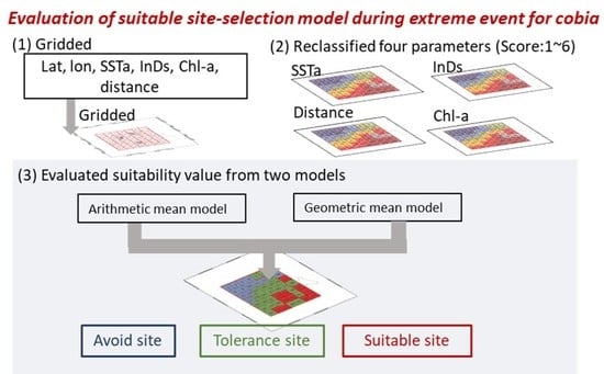
2.3. Suitable Aquaculture Site Selection Model during Extreme Events

2.3.1. Variable Influence Scores and Relative Weighting of Parameters

Four parameters used in the study were reclassified (scored) to create a standard scoring method. Scoring of raw data was based on the threats of extreme events and offshore distance to improve the product quality requirement of cobia cage aquaculture from 1 (least suitable) to 6 (most suitable) (Table 1). Furthermore, the partial least squares regression (PLSR) was used to understand the relative importance of the four parameters during extreme events. The cage culture injury areas (km2) during the cold disasters of 2008 and 2011 in the inner bay of the PHI were collected from the Penghu County Government (Figure 3). PLSR takes into account the latent structure of the predictor variables (injury areas) and the response variables (four parameters), selecting the model of predictor variables that best describes the variation in the response variables [29]. By reducing both the predictor and dependent variables to principal components, PLSR is a useful tool for exploring datasets with large numbers of predictor variables [30]. PLSR analyses were conducted in Statistica 8.0 in our study.
Through the PLSR, variable influence on projection (VIP) scores were produced to assess the relative importance of predictors to the overall models. The scores represent the relative importance of four parameters in representing the variations in injury areas during extreme events. Finally, the relative weighting used in the study was based on the VIP scores proportionally. The SSTA was the most influential (weight = 4), followed by the days of cold-water intrusion (weight = 1), chl-a concentration (weight = 0.8), and offshore distance to the center of the grid (weight = 0.2).

2.3.2. Evaluating Suitable Aquaculture Sites during Extreme Events

After the variable influence scores and relative weighting of the four parameters were determined, an arithmetic mean model (AMM) and a geometric mean model (GMM) were used to evaluate the suitability value (SV) to select the suitable aquaculture sites during extreme events, as presented below:
AMM
S V AMM = 1 n n = 1 n W i S i
GMM
S V GMM = n = 1 n W i S i n
where W i is the relative weighting associated with VIP scores of ith environmental factors during the cold-water disaster, S i is the relative importance variable of ith environmental parameters during the cold-water disaster, and n is the number of all the variables used in this study. Two different model selections of different SV values were also used to estimate the site suitability for each suitable cobia aquaculture selection model. A high SV indicated the more favorable sites for cobia cage aquaculture. Finally, the AMM and the GMM were joined to obtain the SVs in the ranges of 1–2, 2–4, and 4–5 in both models to generate a suitable aquaculture site selection map as avoidance sites, tolerance sites, and suitable sites, respectively, during extreme events.

3. Results

3.1. Variations of 20 °C SST Isotherms in Wintertime around the PHI

The 20 °C isotherms for the monthly mean over thirteen years (2002–2015) and during the winter strong events are displayed in Figure 4. The monthly mean of 20 °C isotherms revealed that the warm KBC water and South China Sea water in January and February surrounded the northern PHI. During El Niño events, the warm water was more northward than the average (Figure 4a,b, red lines). The warm water guided by the Penghu Channel extended more northward and intruded into the northern end of Chang-Yuen Ridge. However, during the La Niña events, the water mass flowed into the western TS along the CCC, and 20 °C isotherms extended to the south of the PHI (Figure 4b, blue lines). However, the El Niño and La Niña events did not always follow the same patterns. For instance, the La Niña events in February 2011 exhibited a northward movement of 20 °C isotherms and did not indicate cold-water intrusion in the PHI (Figure 4b, blue lines).
Therefore, the number of days with wind speed over 6 m/s in the PHI was used as a factor to detect cold-water intrusion events (Table 2). The cumulative durations for strong winds in weak El Niño events (2007) were category C. The highest cumulative durations of category C were in 2006; 2009 was the normal year. These findings suggested that the La Niña events could not be used as a sole factor to detect cold-water intrusion events and suitable aquaculture sites in the PHI. The results indicated that a longer cumulative duration of strong winds led to a lower SSTA in the PHI. The position variations of 20 °C isotherms also supported these findings. The 20 °C isotherms were distributed from north to south of the PHI, categorized into A to C events (Figure 5). We defined category C as cold-water intrusion months.

3.2. Temporal Variations of SSTAs

The monthly mean SSTAs in 2002–2015 for the 49 gridded areas indicated negative values in the northwestern PHI grids 1–20 and 22–24. Positive values were found in the southeastern PHI grids 21 and 25–49 (Figure 6a). The SSTAs in categories A to C were further examined, and the SSTAs in the 49 grids of category A had positive values (Figure 6b). The SSTAs in the 49 grids of category B exhibited similar trends in the monthly mean SSTAs from 2002 to 2015 (Figure 6c). During category C events, all the gridded areas in the inner bay of the PHI displayed negative values (Figure 6d).

3.3. Spatial Distribution of Environmental Parameters Ranked during Extreme Events

The average variable influence scores of four parameters were calculated and rounded in the 49 grids during extreme events (category C). The spatial distributions of monthly SSTAs showed the northern and northwestern PHI had lower scores (1–2) (Figure 7a, grids 1–18). The high scores (5–6) were concentrated in the southern and southeastern PHI (Figure 7a, grids 19–49). The high scores of chl-a were concentrated in the northern PHI (Figure 7b) and the lower scores were located in the central PHI (Figure 7b).
The monthly InDs revealed the different distributed patterns with the SSTA and chl-a concentration. The lower scores occurred in the northwestern and southeastern and southeastern PHI (Figure 7c). The high scores with lower InDs were concentrated in the central and northeastern PHI. The spatial distribution of offshore distance to the PHI coastline showed the grids in the central part of the inner bay and the western parts had a longer distance (Figure 7d).

3.4. Evaluating the Suitable Aquaculture Sites of Cobia in the PHI

During extreme events (category C), the SV distributions of the AMM revealed that the unsuitable areas of lower SV (1–2) were concentrated in the northern and northwestern PHI, and the suitable areas of higher SV (5~6) were concentrated in the southeastern areas (Figure 8a). The SVs of the GMM also revealed the lower SVs in the western and northwestern PHI (Figure 8b), and the higher SVs were located in the central and southeastern areas. According to the joint results of the AMM and the GMM, the suitable aquaculture sites for cobia in extreme events were located in the central and southeastern areas (Figure 8c, red gridded areas). Furthermore, the avoidance sites (Figure 8c, blue gridded areas) should be avoided as the location for cage aquaculture in extreme events. Thus, we suggested that the site of cobia cage aquaculture in the northwestern PHI shown in Figure 1 could move from avoidance sites to the southeastern areas to reduce aquaculture losses and mortality rates.

4. Discussion

Satellite remote sensing is a useful tool for examining coastal waters because of its multi-temporal evaluation [31,32]. In this study, remote sensing data were used intensively to extract biophysical information. The objective of this study was to identify suitable aquaculture sites for cobia in the inner bay of the PHI by using satellite-acquired remotely sensed SST, chl-a, and in situ wind speed data, to reduce aquaculture losses and mortality rates of cobia. The National Oceanic and Atmospheric Administration’s AVHRR satellite infrared SST images have been widely used to study regional fronts since the late 1970s [33]. For over 25 years, these sensors have provided global SST data with 1 km resolution. The instruments scan a swath of approximately 3000 km, which allows frequent observations of the Earth’s surface. AVHRR SST images have long been used to study fisheries and aquacultures, but their accuracy is considerably reduced by cloud coverage. In this study, the cloud coverage in the AVHRR daily images in the winter around the PHI was 20–80%. Microwave observations enable a level of data availability of nearly 100% [34], but the low spatial resolution was not appropriate for use in the coastal areas of the TS. The accuracy of retrieved AVHRR SST was approximately 0.6 °C in the seas around Taiwan [35].
The parameters extracted from the satellite data including SST and chlorophyll-a were surface value measurements [19], while cobia cage aquaculture is grown at about a depth of 4 to 10 m. However, the successful use of SST data in creating spatial temperature gradients rather than absolute temperature values is one of the superior qualities of these data, which could not be achieved by other means [19,36,37]. Studies have indicated that the typical features of SST in winter are the cold water on the northwest side and the blockage of warm water on the southeast side of the TS [29]. The 20 °C isotherm has been suggested as the boundary between the cold CCC and KBC in winter [9,14,35]. Our results further revealed that the average positions of the 20 °C isotherm were in the northern PHI around 23.5°–24°N and displayed annual variations for interaction between cold and warm water. Cold disasters were not isolated events but may have instead been related to La Niña events, with stronger winds leading to an abnormally intensified southwest current in the TS [38].
However, not all the El Niño and La Niña events had the same results in the study, and our results suggested that the La Niña events could not be used to detect cold-water intrusion events and suitable aquaculture sites in the PHI. Furthermore, a study has determined that not all El Niño and La Niña events have the same correlation with SSTs in the TS and suggested that other factors influence the spatial distribution of SSTs [39]. Studies have indicated that the Pacific Decadal Oscillation (PDO) represents the interannual to decadal oscillations in the North Pacific, whereas the ENSO represents the interannual oscillations in the tropical Pacific. The significant correlation between these two indices suggests an interconnection between tropical and subtropical variability in the Pacific [40,41]. The interannual variability in the low latitude western Pacific has been more closely related to the PDO than to the ENSO in recent years. The effect of the ENSO on the northwestern Pacific is not stationary and depends on the phase of the PDO. The relationship between the ENSO and winter monsoon was determined to be weak and nonsignificant in the warm phase of the PDO [42].
The relative weighting of parameters were crucial phases and could have a significant effect on the results when evaluating the SV. Because the assignments are flexible, a variety of scenarios can be generated by some models (e.g., the geographic information system model). To determine these weights, guidance was obtained from a literature review of related species, and from the opinions of experts [8,12]. Faced with many cobia aquaculture indicators during extreme events, the PLSR is one of the useful statistical analysis tools to identify the importance (relative weighting) of the environmental and geographic parameters. The relative weighting used in the study based on the VIP scores of PLSR of the four parameters were SSTA > InDs > chl-a > offshore distance to the PHI coastline. Our results indicated that over 11 days of high-speed winds would lead to cold water intruding into the PHI. A study reported that SST variability was significantly associated with 10-day average wind speeds [43]. When the average wind speed was high, the SST decreased to 14 °C. When wind speed weakened, the SST around the PHI increased rapidly. Wind speed is also an important factor affecting the environmental factors including SST and InDs around the PHI.
The Penghu Channel is located in the eastern PHI and contains inflows from the northward warm KBC [14,44]. The frontal structures also indicated that the Chang-Yuen Ridge partially blocks and diverts water transport [44]. The suitable aquaculture sites for cobia in extreme events selected from the joint results of the AMM and the GMM were located in the central and southeastern areas. These findings revealed that the warm water from the KBC caused higher SST and low InDs. It could help the inner bay of the PHI recover the marine environmental conditions rapidly back to normal during extreme events. Comparing cobia mortality in the extreme events of 2008 around the PHI revealed that the lowest death rates occurred around grids 32–33 and 39–40, which our aquaculture site selection map also indicated was a suitable area for aquaculture sites.
The northwest and south (grids 46–47) of the PHI had high cobia death rates [16]. We also determined that these were unsuitable aquaculture sites for cobia. The Fujian coastal cold water and the cold water from the CCC flow eastward and southward in the TS and reach the Taiwan Bank [39,44]. Therefore, the low SST and InDs recover slowly, causing greater damage to fisheries and aquaculture during extreme events. The ebb and flood tides were considerably larger around the northwestern and southern PHI (grids 45–47), indicating that the water mass changed quickly in a short time. However, in the coastal area of the inner bay (grids 19, 25, and 40), the variation of the ebb and flood tides was smaller, indicating that the ocean conditions changed less rapidly [45]. Furthermore, the areas identified in this study had considerably fewer cold-water InDs, which indicated that they were suitable locations for cobia cage culture. The hydrography of the inner bay was determined using several principal factors, including interaction between the atmosphere and the sea, water exchange with the currents around the PHI, variable topography in the bay, ebb and flood tide changes, accumulation of water because of the prevailing wind-driven circulation, and winter convection [23,43,44].
The distance to the coastline is one of the parameters related to certain logistical problems, including the transportation cost. However, it did not show high relative weighting and could be caused by the narrow landscape of the PHI. In contrast, previous studies had pointed out that the chl-a was also a vitally important factor in aquaculture [19], but the chl-a showed a lower influence as compared to InDs in our study. The cobia cage aquaculture in the PHI is practiced with food, and it could be a human control factor due to an aquaculturist. In contrast to chl-a and offshore distance to the PHI, the SST and InDs directly caused aquaculture losses and mortality rates of cobia during extreme weather events and were not under control. Thus, we paid more attention to the influence of SST and InDs during extreme events in the inner bay of the PHI.

5. Conclusions

In this study, daily marine environmental data were used to develop a suitable aquaculture site selection model for cobia cage aquaculture in the inner bay of the PHI. Elucidating relationships between SST, wind speed, and cumulative duration of wind during extreme events in the PHI was crucial. We classified the situation of the PHI in winter into three categories. Category C was for a monthly cumulative duration of strong winds (>6 m/s) of more than 11 days and was defined as an extreme event (cold-water intrusion disaster event). All the gridded areas had negative values in the inner bay of the PHI in category C. The distribution of low SSTAs was concentrated in the northern and northwestern PHI, and the high SSTAs were concentrated in the southern and southeastern PHI. Low InDs of 15 °C occurred in the central and southern PHI, with the highest number of cumulative days in the northwestern PHI. According to the joint results of the AMM and the GMM to evaluate the aquaculture site selection map during extreme events, the avoidance areas were concentrated in the northern and northwestern PHI, and the suitable areas were concentrated in the southeastern areas. We suggested that the commercial cobia culture operations in the inner bay of the PHI (most of them were located in the tolerance areas) could move to the suitable area to reduce aquaculture losses and mortality rates during extreme events.

Author Contributions

Conceptualization, K.-W.L.; methodology, K.-W.L. and Y.-L.W.; formal analysis, Y.-L.W.; data curation, J.-W.C.; project administration, Y.-L.W.; validation, L.-C.C.; writing—original draft preparation, Y.-L.W.; writing—review and editing, M.-A.L. and K.-W.L.; supervision, K.-W.L. All authors have read and agreed to the published version of the manuscript.

Funding

This research received no external funding.

Acknowledgments

This study was financially supported by the Penghu County Government (108-2929-I-019-001-MY4) and the National Science Council (MOST 106-2611-M-019-012 and MOST 107-2611-M-019-017).

Conflicts of Interest

The authors declare no conflict of interest.

References

  1. The FAO Fisheries and Aquaculture Department. The State of World Fisheries and Aquaculture; Food and Agriculture Organization of the United Nations: Rome, Italy, 2012; pp. 3–5. [Google Scholar]
  2. Bondad-Reantaso, M.G.; Arthur, J.R.; Subasinghe, R.P. Understanding and Applying Risk Analysis in Aquaculture; Food and Agriculture Organization of the United Nations: Rome, Italy, 2008. [Google Scholar]
  3. Liu, Y.; Saitoh, S.I.; Radiarta, I.N.; Igarashi, H.; Hirawake, T. Spatiotemporal variations in suitable areas for Japanese scallop aquaculture in the Dalian coastal area from 2003 to 2012. Aquaculture 2014, 422, 172–183. [Google Scholar] [CrossRef] [Green Version]
  4. FAO. The State of World Fisheries and Aquaculture 2018; Food and Agriculture Organization of United Nations: Rome, Italy, 2018; p. 227. [Google Scholar]
  5. De Silva, S.S.; Soto, D. Climate change and aquaculture: Potential impacts, adaptation and mitigation. Climate change implications for fisheries and aquaculture: Overview of current scientific knowledge. FAO Fish. Aquac. Tech. Pap. 2009, 530, 151–212. [Google Scholar]
  6. Shaffer, R.V.; Nakamura, E.L. Synopsis of Biological Data on the Cobia Rachycentron canadum (Pisces: Rachycentridae); NOAA Technical Report NMFS; NOAA/National Marine Fisheries Service: Silver Spring, MD, USA, 1989.
  7. Ditty, J.G. Larval development, distribution, and ecology of cobia Rachycentron canadum (family: Rachycentridae), in the northern Gulf of Mexico. Fish. Bull. 1992, 96, 223–236. [Google Scholar]
  8. Liao, I.C.; Leano, E.M. Cobia Aquaculture: Research, Development and Commercial Production; Food and Agriculture Organization of the United Nations: Rome, Italy, 2007; pp. 131–145. [Google Scholar]
  9. Chang, Y.; Lee, K.T.; Lee, M.A.; Lan, K.W. Satellite Observation on the Exceptional Intrusion of Cold Water in the Taiwan Strait. Terr. Atmos. Ocean. Sci. 2009, 20. [Google Scholar] [CrossRef]
  10. Huang, T.S.; Lin, K.J.; Chen, C.C.; Tsai, W.S. Study on cobia, Rachycentron canadum, over-wintering using the indoor high-density recirculating system. J. Taiwan Fish Res. 2002, 10, 53–62. [Google Scholar]
  11. Huang, C.T.; Miao, S.; Farok, A. Economic analysis of cobia’s (Rachentron canadum) phase nursery stage culture in Taiwan. J. Fish Soc. Taiwan. 2008, 35, 117–130. [Google Scholar]
  12. Miao, S.; Jen, C.C.; Huang, C.T.; Hu, S.H. Ecological and economic analysis for cobia Rachycentron canadum commercial cage culture in Taiwan. Aquac. Int. 2009, 17, 125–141. [Google Scholar] [CrossRef]
  13. Sun, L.; Chen, H.; Huang, L.; Wang, Z.; Yan, Y. Growth and energy budget of juvenile cobia (Rachycentron canadum) relative to ration. Aquaculture 2006, 257, 214–220. [Google Scholar] [CrossRef]
  14. Jan, S.; Wang, J.; Chern, C.S.; Chao, S.Y. Seasonal variation of the circulation in the Taiwan Strait. J. Mar. Syst. 2002, 35, 249–2688. [Google Scholar] [CrossRef]
  15. Kuo, N.J.; Ho, C.R. ENSO effect on the sea surface wind and sea surface temperature in the Taiwan Strait. Res. Lett. 2004, 31. [Google Scholar] [CrossRef]
  16. Lee, M.A.; Yang, Y.C.; Shen, Y.L.; Chang, Y.; Tsai, W.S.; Lan, K.W.; Kuo, Y.C. Effects of an Unusual Cold-Water Intrusion in 2008 on the Catch of Coastal Fishing Methods around Penghu Islands, Taiwan. Terr. Atmos. Ocean. Sci. 2014, 25, 107–120. [Google Scholar] [CrossRef] [Green Version]
  17. Qiu, F.; Fang, W.; Fang, Y.; Guo, P. Anomalous oceanic characteristics in the South China Sea associated with the large-scale forcing during 2006–2009. J. Mar. Syst. 2012, 100, 9–18. [Google Scholar] [CrossRef]
  18. Radiarta, I.N.; Saitoh, S.I.; Miyazono, A. GIS-based multi-criteria evaluation models for identifying suitable sites for Japanese scallop (Mizuhopecten yessoensis) aquaculture in Funka Bay, southwestern Hokkaido, Japan. Aquaculture 2008, 284, 127–135. [Google Scholar] [CrossRef]
  19. Radiarta, I.N.; Saitoh, S.I. Biophysical models for Japanese scallop, Mizuhopecten yessoensis, aquaculture site selection in Funka Bay, Hokkaido, Japan, using remotely sensed data and geographic information system. Aquac. Int. 2009, 17, 403–419. [Google Scholar] [CrossRef]
  20. Saitoh, S.I.; Mugo, R.; Radiarta, I.N.; Asaga, S.; Takahashi, F.; Hirawake, T.; Shima, S. Some operational uses of satellite remote sensing and marine GIS for sustainable fisheries and aquaculture. ICES J. Mar. Sci. 2011, 68, 687–695. [Google Scholar] [CrossRef] [Green Version]
  21. Lee, M.A.; Yeah, C.D.; Cheng, C.H.; Chan, J.W.; Lee, K.T. Empirical orthogonal function analysis of AVHRR sea surface temperature patterns in Taiwan Strait. J. Mar. Sci. Technol. 2003, 11, 1–7. [Google Scholar]
  22. McClain, E.P.; Pichel, W.G.; Walton, C.C. Comparative performance of AVHRR-based multichannel sea surface temperatures. J. Geophys. Res. Oceans 1985, 90, 11587–11601. [Google Scholar] [CrossRef]
  23. Jan, S.; Chao, S.Y. Seasonal variation of volume transport in the major inflow region of the Taiwan Strait: The Penghu Channel. Deep-Sea Res. Part II-Top. Stud. Oceanogr. 2003, 50, 1117–1126. [Google Scholar] [CrossRef]
  24. Hsieh, H.J.; Hsien, Y.L.; Jeng, M.S.; Tsai, W.S.; Su, W.C.; Chen, C.A. Tropical fishes killed by the cold. Coral Reefs 2008, 27, 599. [Google Scholar] [CrossRef]
  25. Huang, B.; Banzon, V.F.; Freeman, E.; Lawrimore, J.; Liu, W.; Peterson, T.C.; Smith, T.M.; Thorne, P.W.; Woodruff, S.D.; Zhang, H.-M. Extended Reconstructed Sea Surface Temperature Version 4 (ERSST.v4). Part I: Upgrades and Intercomparisons. J. Clim. 2015, 28, 911–930. [Google Scholar] [CrossRef] [Green Version]
  26. Ueng, P.S.; Yu, S.L.; Tzeng, J.J.; Ou, C.H. The effect of water temperature on growth rate of cobia Rachycentron canadum in Penghu. In Proceedings of the 6th Asian Fisheries Forum, Kaohsiung, Taiwan, 25–30 November 2001. [Google Scholar]
  27. Kirby-Smith, W.W.; Barber, R.T. Suspension-feeding aquaculture systems: Effects of phytoplankton concentration and temperature on growth of the bay scallop. Aquaculture 1974, 3, 135–145. [Google Scholar] [CrossRef]
  28. Theobald, D.M.; Norman, J.B.; Peterson, E.; Ferraz, S.; Wade, A.; Sherburne, M.R. Functional Linkage of Water Basins and STREAMS (FLoWS) v1 User’s Guide: ArcGIS Tools for Network-Based Analysis of Freshwater Ecosystems; Natural Resource Ecology Lab, Colorado State University: Fort Collins, CO, USA, 2006; p. 43. [Google Scholar]
  29. Wold, S.; Sjöström, M.; Eriksson, L. PLS-regression: A basic tool of chemometrics. Chemom. Intell. Lab. Syst. 2001, 58, 109–130. [Google Scholar] [CrossRef]
  30. Carrascal, L.M.; Galván, I.; Gordo, O. Partial least squares regression as an alternative to current regression methods used in ecology. Oikos 2009, 118, 681–690. [Google Scholar] [CrossRef]
  31. Kapetsky, J.M.; McGregor, L.; Nanne, E.H. Geographical Information System and Satellite Remote Sensing to Plant for Aquaculture Development; Food and Agriculture Organization of the United Nations: Rome, Italy, 1987. [Google Scholar]
  32. Meaden, G.J. Geographical Information Systems and Remote Sensing in Inland Fisheries and Aquaculture; No. F009. 048; FAO: Rome, Italy, 1991. [Google Scholar]
  33. Legeckis, R. A survey of worldwide sea surface temperature fronts detected by environmental satellites. J. Geophys. Res. 1978, 83, 4501–4522. [Google Scholar] [CrossRef]
  34. Hosoda, K. A review of satellite-based microwave observation of sea surface temperature. J. Oceanogr. 2010, 66, 439–473. [Google Scholar] [CrossRef]
  35. Lee, M.A.; Chang, Y.; Lee, K.T.; Chan, J.W.; Liu, D.C.; Su, W.C. A satellite and field view of the winter SST variability in the Taiwan Strait. In Proceedings of the 2005 IEEE International Geoscience and Remote Sensing Symposium, IGARSS′05, Seoul, Korea, 29 July 2005; pp. 2621–2626. [Google Scholar]
  36. Gentemann, C.L.; Donlon, C.J.; Stuart-Menteth, A.; Wentz, F.J. Diurnal signals in satellite sea surface temperature measurements. Geophys. Res. Lett. 2003, 30, 30. [Google Scholar] [CrossRef] [Green Version]
  37. Perez, O.M.; Telfer, T.C.; Ross, L.G. Geographical information systems-based models for offshore floating marine fish cage aquaculture site selection in Tenerife, Canary Islands. Aquac. Res. 2005, 36, 946–961. [Google Scholar] [CrossRef]
  38. Liao, E.; Jiang, Y.; Li, L.; Hong, H.; Yan, X. The cause of the 2008 cold disaster in the Taiwan Strait. Ocean Model 2013, 62, 1–10. [Google Scholar] [CrossRef]
  39. Tzeng, M.T.; Lan, K.W.; Chan, J.W. Interannual variability of wintertime sea surface temperatures in the eastern Taiwan Strait. J. Mar. Sci. Technol. Taiwan 2012, 20, 707–712. [Google Scholar]
  40. Zhang, R.-H.; Rothstein, L.M.; Busalacchi, A.J. Origin of upper-ocean warming and El Nino change on decadal scales in the tropical Pacific Ocean. Nature 1998, 391, 879–883. [Google Scholar] [CrossRef]
  41. Newman, M.; Compo, G.P.; Alexander, M.A. ENSO-forced variability of the Pacific decadal oscillation. J. Clim. 2003, 16, 3853–3857. [Google Scholar] [CrossRef] [Green Version]
  42. Wu, C.R. Interannual modulation of the Pacific Decadal Oscillation (PDO) on the low-latitude western North Pacific. Prog. Oceanogr. 2013, 110, 49–58. [Google Scholar] [CrossRef]
  43. Cheng, Y.H.; Chang, M.H. Exceptionally cold water days in the southern Taiwan Strait: Their predictability and relation to La Niña. Nat. Hazards Earth Syst. Sci. 2018, 18. [Google Scholar] [CrossRef] [Green Version]
  44. Chang, Y.; Shimada, T.; Lee, M.A.; Lu, H.J.; Sakaida, F.; Kawamura, H. Wintertime sea surface temperature fronts in the Taiwan Strait. Geophys. Res. Lett. 2006, 33. [Google Scholar] [CrossRef]
  45. Shih, Y.C. Integrated GIS and AHP for marine aquaculture site selection in Penghu Cove in Taiwan. J. Coast. Zone Manag. 2017, 20, 438. [Google Scholar] [CrossRef] [Green Version]
Figure 1. (a) Map of the bottom topography and flow patterns in winter. The gray contours indicate coastlines and bottom depth in meters. CYR, PHI, and PHC represent the locations of the Chang-Yuen Ridge, Penghu Islands, and Penghu Channel, respectively. The gray and black arrows indicate the China Coastal Current (CCC) and Kuroshio Branch Current (KBC) (redrawn from [14]). (b) Study area and regional divisions; the gold star is the gauge station and black marks are the cobia cage culture locations in the PHI. The pixel of each grid is 0.025°.
Remotesensing 12 02689 g001
Figure 2. Schematic of the evaluation of site selection maps for cobia cage culture in the inner bay of the Penghu Islands.
Remotesensing 12 02689 g002
Figure 3. (a) Histogram of high-speed wind days (>6 m/s) during the wintertime (January and February) from 2002 to 2015 in the Penghu Islands. (b) The injury areas during the extreme events of cold disaster (2008 and 2011) of 49 grids.
Remotesensing 12 02689 g003
Figure 4. Contours of 20 °C isotherms of (a) 13-year average (black line), El Niño events average (red lines), and La Niña events average (blue lines) during January, and (b) 13-year average (black line), El Niño events (red lines), and La Niña events (blue lines) during February. The red box indicates the study area of the Penghu Islands.
Remotesensing 12 02689 g004
Figure 5. Contours of 20 °C isotherms in the Taiwan Strait (TS) during the case studies of (a) category A, (b) category B, and (c) category C during winter.
Remotesensing 12 02689 g005
Figure 6. Time series of SSTAs for 49 grids (a) during 2002–2015, (b) for category A, (c) for category B, and (d) for category C. Red columns represent positive SSTAs and blue columns represent negative SSTAs. The lower grid cell numbers occur in the northern part of the PHI, with higher numbers towards the southern part of the study area.
Remotesensing 12 02689 g006
Figure 7. Spatial distributions of the average variable influence scores of (a) SST anomalies (SSTAs), (b) chlorophyll-a (chl-a) concentration (c) cold-water (<15 °C) intrusion days (InDs), and (d) offshore distance from the PHI coastline map for all 49 gridded areas in the inner bay of the PHI during extreme events (category C).
Remotesensing 12 02689 g007
Figure 8. Spatial distributions of the two types of model selection proportion scales for (a) the arithmetic mean model (AMM) and (b) the geometric mean model (GMM). (c) The overlapped results of the two models selected. The avoidance sites are the blue areas. The tolerance sites are the green areas. The suitable sites are the red areas.
Remotesensing 12 02689 g008
Table 1. The standard of variable influence scores of the four parameters used in this study.
Parameter654321
Sea surface temperature anomalies 0.78~0.490.49~0.230.23~−0.08−0.08~−0.3−0.3~−0.8−0.8~−1.08
Cold water intrusion day8910111213-16
Chlorophyll a 1.4~1.351.35~1.331.33~1.321.32~1.301.30~1.281.28~1.24
Distance to coastal line20~180190~430430~600600~12601260~23002300~3900
Table 2. The result of reclassification by strong speed wind days. Category A (the strong speed wind day for 1–6 days), category B (7–11 days), and category C (over 11 days).
CategoryYearMonthAverage SSTStrong Wind SpeedENSO Event
A2002122.684Normal year
2002221.503Normal year
2003220.765El Nino (Moderate)
2007219.242El Nino (Weak)
2009220.713Normal year
2010120.696El Nino (Moderate)
2010221.366El Nino (Moderate)
2011214.756La Nina (Strong)
2014220.455El Nino (Weak)
2015220.224El Nino (Strong)
B2003120.359El Nino (Moderate)
2004119.6010El Nino (Weak)
2004220.169El Nino (Weak)
2005118.2311La Nina (Weak)
2005217.248La Nina (Weak)
2006116.8810Normal year
2013121.3111Normal year
2013218.799Normal year
2014120.648El Nino (Weak)
2015119.478El Nino (Strong)
C2006219.8012Normal year
2007121.9214El Nino (Weak)
2008120.9414La Nina (Strong)
2008217.9118La Nina (Strong)
2009121.9713Normal year
2011118.1520La Nina (Strong)
2012117.3013La Nina (Moderate)
2012217.0613La Nina (Moderate)

