An Operational Split-Window Algorithm for Retrieving Land Surface Temperature from Geostationary Satellite Data: A Case Study on Himawari-8 AHI Data

 , , and
Abstract
1. Introduction
2. Methodology
2.1. LST Retrieval Algorithm
2.2. LSE Estimation
3. Experimental Data and Validation Strategy
3.1. Himawari-8/AHI Data
3.2. ERA5 Atmospheric Reanalysis Data
3.3. MODIS Product
3.4. Validation Strategy
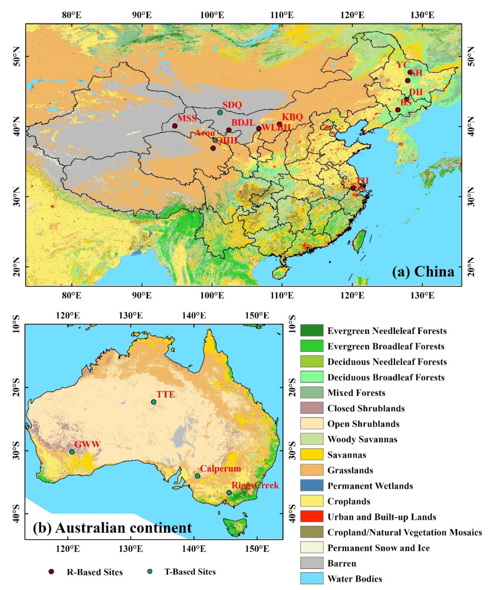
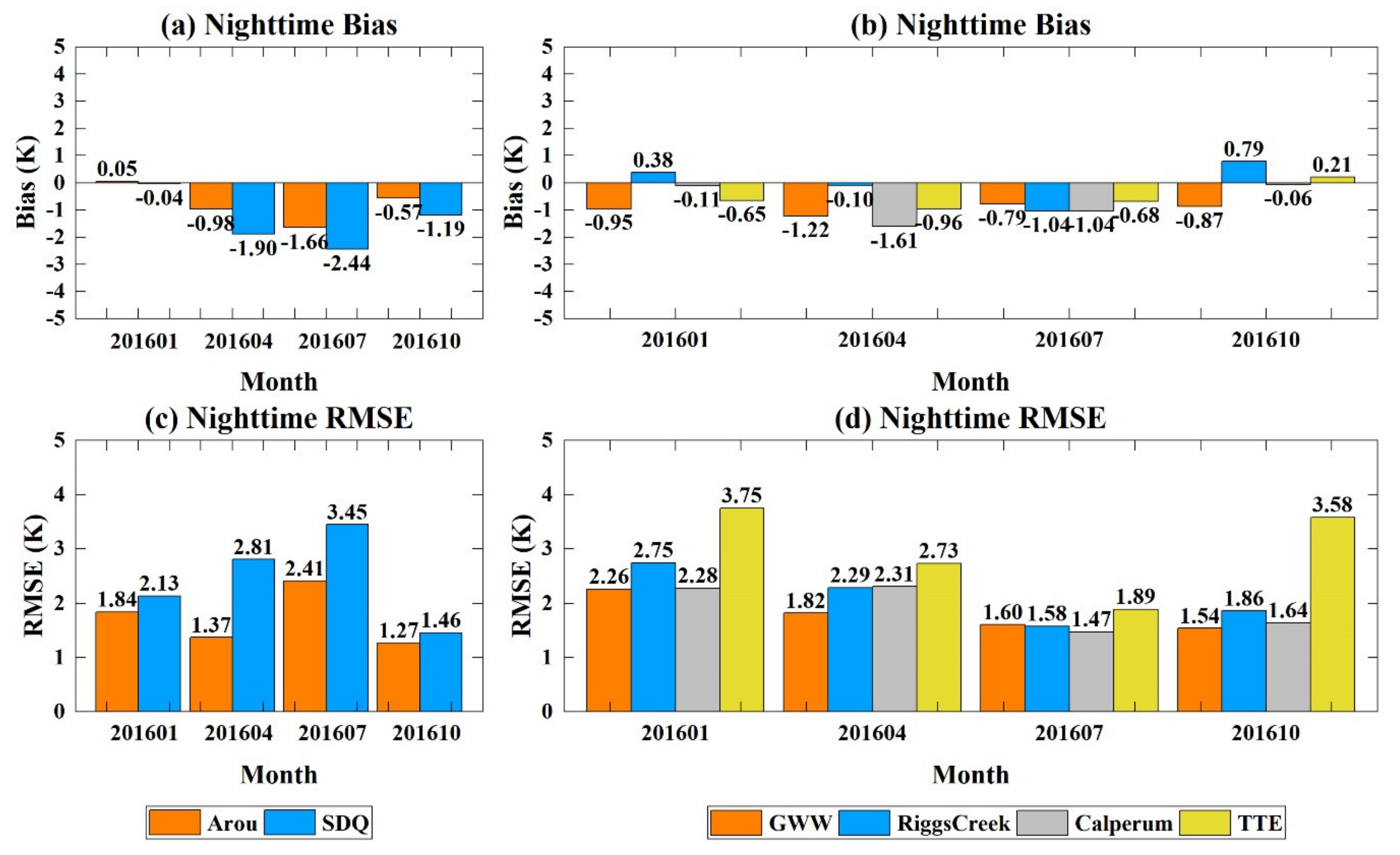
3.4.1. T-Based Validation
3.4.2. R-Based Validation
3.4.3. Intercomparison Validation
4. Results
4.1. T-Based Validation Results
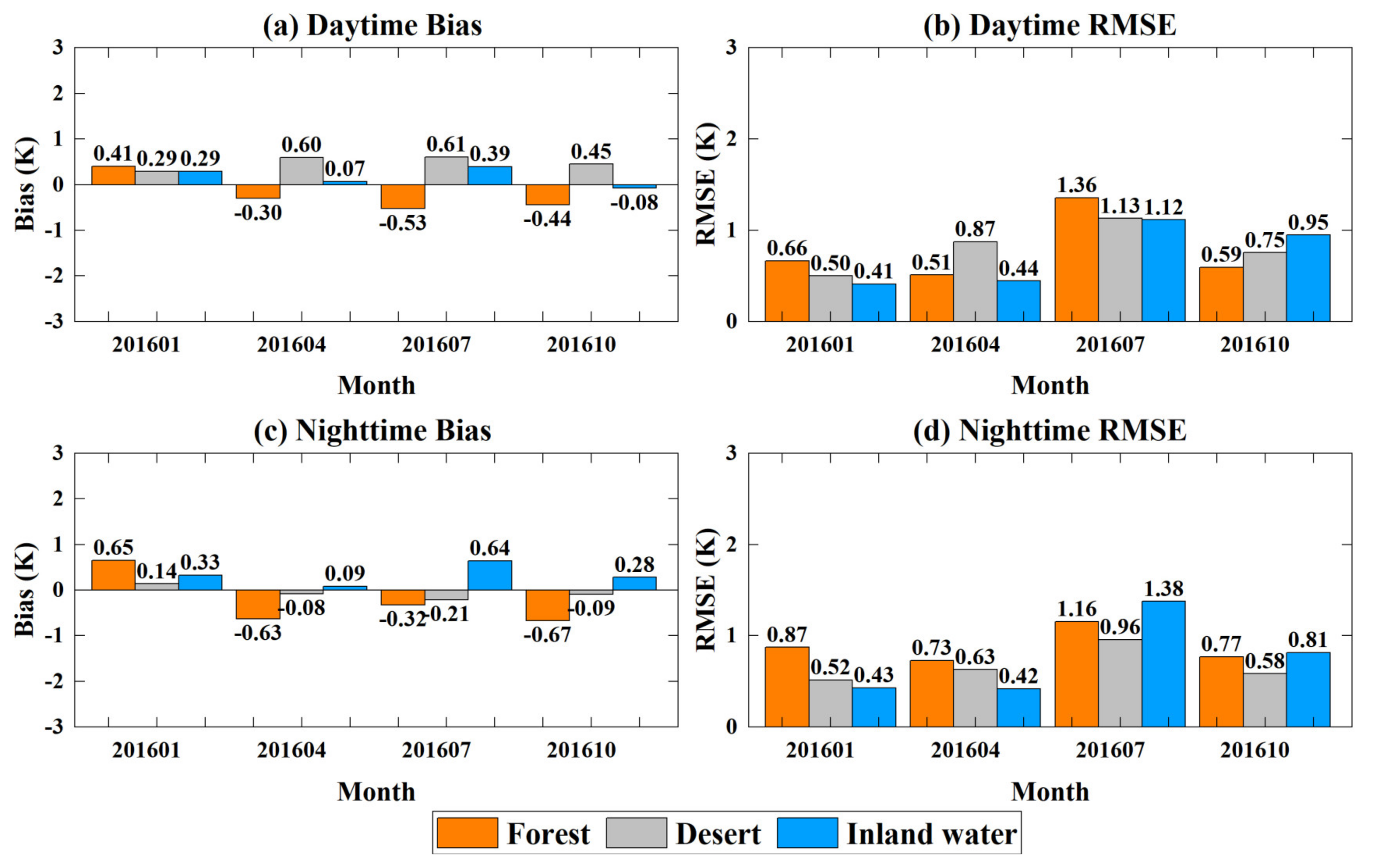
4.2. R-Based Validation Results
4.3. Intercomparison Validation of Results
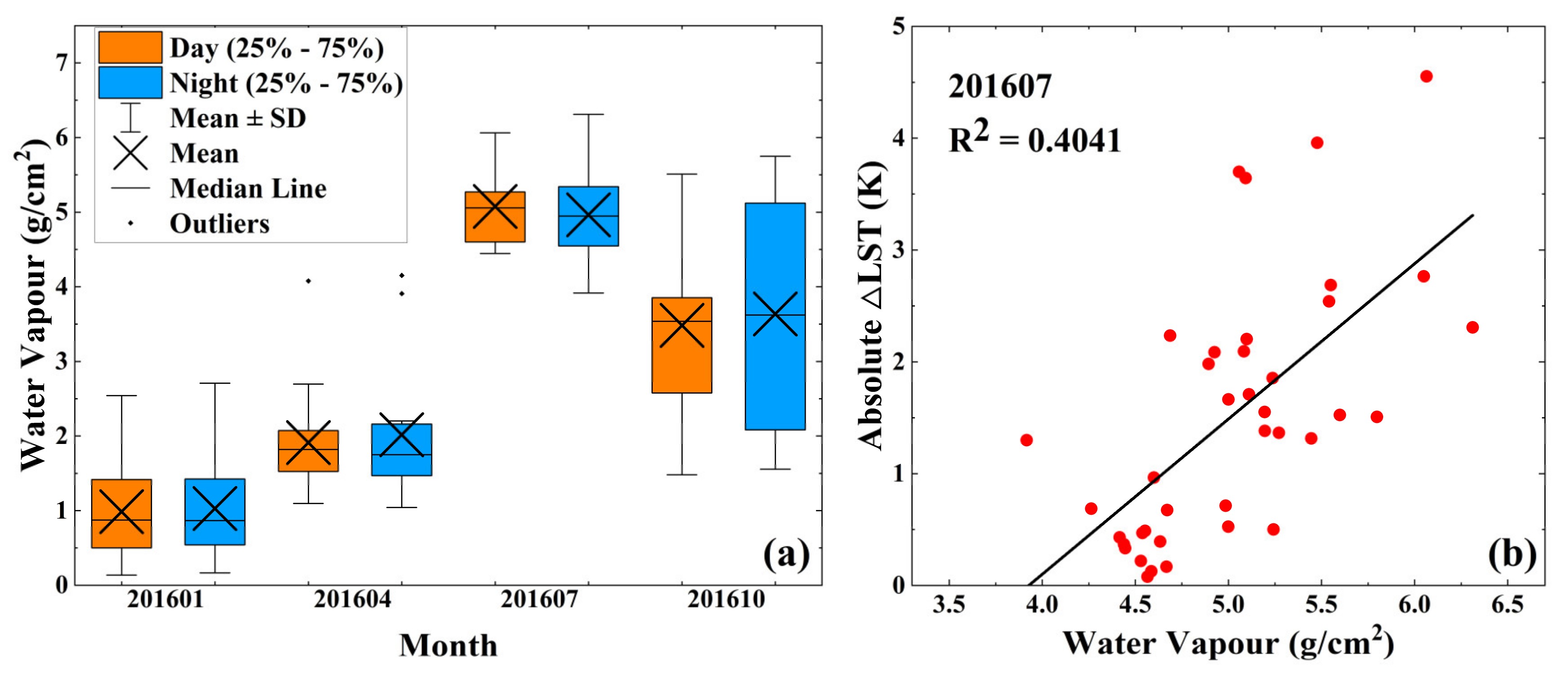
5. Discussion
6. Conclusions
Author Contributions
Funding
Acknowledgments
Conflicts of Interest
References
- Li, Z.; Tang, B.; Wu, H.; Ren, H.; Yan, G.; Wan, Z.; Trigo, I.F.; Sobrino, J.A. Satellite-derived land surface temperature: Current status and perspectives. Remote Sens. Environ. 2013, 131, 14–37. [Google Scholar] [CrossRef]
- Cao, B.; Liu, Q.; Du, Y.; Roujean, J.-L.; Gastellu-Etchegorry, J.-P.; Trigo, I.F.; Zhan, W.; Yu, Y.; Cheng, J.; Jacob, F.; et al. A review of earth surface thermal radiation directionality observing and modeling: Historical development, current status and perspectives. Remote Sens. Environ. 2019, 232, 111304. [Google Scholar] [CrossRef]
- Yamamoto, Y.; Ishikawa, H. Influence of urban spatial configuration and sea breeze on land surface temperature on summer clear-sky days. Urban Clim. 2020, 31, 100578. [Google Scholar] [CrossRef]
- Yamamoto, Y.; Ishikawa, H. Spatiotemporal Variability Characteristics of Clear-Sky Land Surface Temperature in Urban Areas of Japan Observed by Himawari-8. SOLA 2018, 14, 179–184. [Google Scholar] [CrossRef]
- Hu, T.; Renzullo, L.J.; Dijk, A.I.; He, J.; Tian, S.; Xu, Z.; Zhou, J.; Liu, T.; Liu, Q. Monitoring agricultural drought in Australia using MTSAT-2 land surface temperature retrievals. Remote Sens. Environ. 2020, 236, 1–13. [Google Scholar] [CrossRef]
- Hu, T.; Dijk, A.I.; Renzullo, L.J.; Xu, Z.; He, J.; Tian, S.; Zhou, J.; Li, H. On agricultural drought monitoring in Australia using Himawari-8 geostationary thermal infrared observations. Int. J. Appl. Earth Obs. Geoinf. 2020, 91, 1–13. [Google Scholar] [CrossRef]
- Mcmillin, L.M. Estimation of Sea Surface Temperatures from Two Infrared Window Measurements with Different Absorption. J. Geophys. Res. 1975, 80, 5113–5117. [Google Scholar] [CrossRef]
- Qin, Z.; Karnieli, A.; Berliner, P. A mono-window algorithm for retrieving land surface temperature from Landsat TM data and its application to the Israel-Egypt border region. Int. J. Remote Sens. 2001, 22, 3719–3746. [Google Scholar] [CrossRef]
- Sun, D.; Pinker, R.T. Estimation of land surface temperature from a Geostationary Operational Environmental Satellite (GOES-8). J. Geophys. Res. Atmos. 2003, 108. [Google Scholar] [CrossRef]
- Sun, D.; Pinker, R.T. Retrieval of surface temperature from the MSG-SEVIRI observations: Part I. Methodology. Int. J. Remote Sens. 2007, 28, 5255–5272. [Google Scholar] [CrossRef]
- Yamamoto, Y.; Ishikawa, H.; Oku, Y.; Hu, Z. An Algorithm for Land Surface Temperature Retrieval Using Three Thermal Infrared Bands of Himawari-8. J. Meteorol. Soc. Jpn. Ser. II 2018, 96, 59–76. [Google Scholar] [CrossRef]
- Sobrino, J.A.; Caselles, V.; Coll, C. Theoretical split-window algorithms for determining the actual surface temperature. II Nuovo Cim. C 1993, 16, 219–236. [Google Scholar] [CrossRef]
- Gillespie, A.; Rokugawa, S.; Matsunaga, T.; Cothern, J.S.; Hook, S.; Kahle, A.B. A temperature and emissivity separation algorithm for Advanced Spaceborne Thermal Emission and Reflection Radiometer (ASTER) images. IEEE Trans. Geosci. Remote Sens. 1998, 36, 1113–1126. [Google Scholar] [CrossRef]
- Wan, Z.; Dozier, J. A generalized split-window algorithm for retrieving land-surface temperature from space. IEEE Trans. Geosci. Remote Sens. 1996, 34, 892–905. [Google Scholar] [CrossRef]
- Wan, Z.; Li, Z. A physics-based algorithm for retrieving land-surface emissivity and temperature from EOS/MODIS data. IEEE Trans. Geosci. Remote Sens. 1997, 35, 980–996. [Google Scholar] [CrossRef]
- Islam, T.; Hulley, G.C.; Malakar, N.K.; Radocinski, R.G.; Guillevic, P.C.; Hook, S.J. A Physics-Based Algorithm for the Simultaneous Retrieval of Land Surface Temperature and Emissivity from VIIRS Thermal Infrared Data. IEEE Trans. Geosci. Remote Sens. 2016, 55, 563–576. [Google Scholar] [CrossRef]
- Li, H.; Sun, D.; Yu, Y.; Wang, H.; Liu, Y.; Liu, Q.; Du, Y.; Wang, H.; Cao, B. Evaluation of the VIIRS and MODIS LST products in an arid area of Northwest China. Remote Sens. Environ. 2014, 142, 111–121. [Google Scholar] [CrossRef]
- Yu, Y.; Privette, J.L.; Pinheiro, A.C.T. Evaluation of Split-Window Land Surface Temperature Algorithms for Generating Climate Data Records. IEEE Trans. Geosci. Remote Sens. 2008, 46, 179–192. [Google Scholar] [CrossRef]
- Tang, B.; Bi, Y.; Li, Z.; Xia, J. Generalized Split-Window Algorithm for Estimate of Land Surface Temperature from Chinese Geostationary FengYun Meteorological Satellite (FY-2C) Data. Sensors 2008, 8, 933–951. [Google Scholar] [CrossRef]
- Gao, C.; Tang, B.; Wu, H.; Jiang, X.; Li, Z. A generalized split-window algorithm for land surface temperature estimation from MSG-2/SEVIRI data. Int. J. Remote Sens. 2013, 34, 4182–4199. [Google Scholar] [CrossRef]
- Trigo, I.F. Land surface temperature from multiple geostationary satellites. Int. J. Remote Sens. 2013, 34, 3051–3068. [Google Scholar] [CrossRef]
- Liu, Y.; Yu, Y.; Yu, P.; Wang, H.; Rao, Y. Enterprise LST Algorithm Development and Its Evaluation with NOAA 20 Data. Remote Sens. 2019, 11, 2003. [Google Scholar] [CrossRef]
- Tang, B.; Shao, K.; Li, Z.; Wu, H.; Nerry, F.; Zhou, G. Estimation and Validation of Land Surface Temperatures from Chinese Second-Generation Polar-Orbit FY-3A VIRR Data. Remote Sens. 2015, 7, 3250–3273. [Google Scholar] [CrossRef]
- Qin, Z.; Dall’Olmo, G.; Karnieli, A.; Berliner, P. Derivation of split window algorithm and its sensitivity analysis for retrieving land surface temperature from NOAA-advanced very high resolution radiometer data. J. Geophys. Res. Atmos. 2001, 106, 22655–22670. [Google Scholar] [CrossRef]
- Jiang, J.; Li, H.; Liu, Q.; Wang, H.; Du, Y.; Cao, B.; Zhong, B.; Wu, S. Evaluation of land surface temperature retrieval from FY-3B/VIRR data in an arid area of northwestern China. Remote Sens. 2015, 7, 7080–7104. [Google Scholar] [CrossRef]
- Wang, M.; He, G.; Zhang, Z.; Wang, G.; Wang, Z.; Yin, R.; Cui, S.; Wu, Z.; Cao, X. A radiance-based split-window algorithm for land surface temperature retrieval: Theory and application to MODIS data. Int. J. Appl. Earth Obs. Geoinf. 2019, 76, 204–217. [Google Scholar] [CrossRef]
- Snyder, W.C.; Wan, Z.; Zhang, Y.; Feng, Y. Classification-based emissivity for land surface temperature measurement from space. Int. J. Remote Sens. 1998, 19, 2753–2774. [Google Scholar] [CrossRef]
- Valor, E.; Caselles, V. Mapping land surface emissivity from NDVI: Application to European, African, and South American areas. Remote Sens. Environ. 1996, 57, 167–184. [Google Scholar] [CrossRef]
- Yamamoto, Y.; Ishikawa, H. Thermal Land Surface Emissivity for Retrieving Land Surface Temperature from Himawari-8. J. Meteorol. Soc. Jpn. Ser. II 2018, 96B, 43–58. [Google Scholar] [CrossRef]
- Seemann, S.W.; Borbas, E.E.; Knuteson, R.O.; Stephenson, G.R.; Huang, H.-L. Development of a global infrared land surface emissivity database for application to clear sky sounding retrievals from multispectral satellite radiance measurements. J. Appl. Meteorol. Climatol. 2008, 47, 108–123. [Google Scholar] [CrossRef]
- Duan, S.; Li, Z.; Cheng, J.; Leng, P. Cross-satellite comparison of operational land surface temperature products derived from MODIS and ASTER data over bare soil surfaces. ISPRS J. Photogramm. Remote Sens. 2017, 126, 1–10. [Google Scholar] [CrossRef]
- Duan, S.; Li, Z.; Li, H.; Göttsche, F.-M.; Wu, H.; Zhao, W.; Leng, P.; Zhang, X.; Coll, C. Validation of Collection 6 MODIS land surface temperature product using in situ measurements. Remote Sens. Environ. 2019, 225, 16–29. [Google Scholar] [CrossRef]
- Olioso, A. Simulating the relationship between thermal emissivity and the normalized difference vegetation index. Int. J. Remote Sens. 1995, 16, 3211–3216. [Google Scholar] [CrossRef]
- Hulley, G.C.; Hook, S.J.; Abbott, E.; Malakar, N.; Islam, T.; Abrams, M. The ASTER Global Emissivity Dataset (ASTER GED): Mapping Earth’s emissivity at 100 meter spatial scale. Geophys. Res. Lett. 2015, 42, 7966–7976. [Google Scholar] [CrossRef]
- Li, H.; Yang, Y.; Li, R.; Wang, H.; Cao, B.; Bian, Z.; Hu, T.; Du, Y.; Sun, L.; Liu, Q. Comparison of the MuSyQ and MODIS Collection 6 land surface temperature products over barren surfaces in the Heihe River basin, China. IEEE Trans. Geosci. Remote Sens. 2019, 57, 8081–8094. [Google Scholar] [CrossRef]
- Meng, X.; Li, H.; Du, Y.; Liu, Q.; Zhu, J.; Sun, L. Retrieving land surface temperature from landsat 8 TIRS data using RTTOV and ASTER GED. In Proceedings of the 2016 IEEE International Geoscience and Remote Sensing Symposium (IGARSS), Beijing, China, 10–15 July 2016; pp. 4302–4305. [Google Scholar]
- Duan, S.; Li, Z.; Wang, C.; Zhang, S.; Tang, B.; Leng, P.; Gao, M. Land-surface temperature retrieval from Landsat 8 single-channel thermal infrared data in combination with NCEP reanalysis data and ASTER GED product. Int. J. Remote Sens. 2019, 40, 1763–1778. [Google Scholar] [CrossRef]
- Zhang, S.; Duan, S.; Li, Z.; Huang, C.; Wu, H.; Han, X.; Leng, P.; Gao, M. Improvement of Split-Window Algorithm for Land Surface Temperature Retrieval from Sentinel-3A SLSTR Data Over Barren Surfaces Using ASTER GED Product. Remote Sens. 2019, 11, 3025. [Google Scholar] [CrossRef]
- Wang, H.; Yu, Y.; Yu, P.; Liu, Y. Land Surface Emissivity Product for NOAA JPSS and GOES-R Missions: Methodology and Evaluation. IEEE Trans. Geosci. Remote Sens. 2020, 58, 307–318. [Google Scholar] [CrossRef]
- Li, H.; Wang, H.; Yang, Y.; Du, Y.; Cao, B.; Bian, Z.; Liu, Q. Evaluation of Atmospheric Correction Methods for the ASTER Temperature and Emissivity Separation Algorithm Using Ground Observation Networks in the HiWATER Experiment. IEEE Trans. Geosci. Remote Sens. 2019, 57, 3001–3014. [Google Scholar] [CrossRef]
- Sekertekin, A.; Bonafoni, S. Land Surface Temperature Retrieval from Landsat 5, 7, and 8 over Rural Areas: Assessment of Different Retrieval Algorithms and Emissivity Models and Toolbox Implementation. Remote Sens. 2020, 12, 294. [Google Scholar] [CrossRef]
- Wang, L.; Lu, Y.; Yao, Y. Comparison of Three Algorithms for the Retrieval of Land Surface Temperature from Landsat 8 Images. Sensors 2019, 19, 5049. [Google Scholar] [CrossRef] [PubMed]
- Yu, W.; Ma, M.; Li, Z.; Tan, J.; Wu, A. New Scheme for validating remote-sensing land surface temperature products with station observations. Remote Sens. 2017, 9, 1210. [Google Scholar] [CrossRef]
- Duan, S.; Li, Z.; Wu, H.; Leng, P.; Gao, M.; Wang, C. Radiance-based validation of land surface temperature products derived from Collection 6 MODIS thermal infrared data. Int. J. Appl. Earth Obs. Geoinf. 2018, 70, 84–92. [Google Scholar] [CrossRef]
- Hulley, G.C.; Hughes, C.G.; Hook, S.J. Quantifying uncertainties in land surface temperature and emissivity retrievals from ASTER and MODIS thermal infrared data. J. Geophys. Res. Atmos. 2012, 117, 1–18. [Google Scholar] [CrossRef]
- Yu, W.; Ma, M.; Yang, H.; Tan, J.; Li, X. Supplement of the radiance-based method to validate satellite-derived land surface temperature products over heterogeneous land surfaces. Remote Sens. Environ. 2019, 230, 111188. [Google Scholar] [CrossRef]
- Choi, Y.-Y.; Suh, M.-S. Development of Himawari-8/Advanced Himawari Imager (AHI) Land Surface Temperature Retrieval Algorithm. Remote Sens. 2018, 10, 2013. [Google Scholar] [CrossRef]
- Duan, S.; Li, Z. Intercomparison of operational land surface temperature products derived from MSG-SEVIRI and Terra/Aqua-MODIS data. IEEE J. Sel. Top. Appl. Earth Obs. Remote Sens. 2015, 8, 4163–4170. [Google Scholar] [CrossRef]
- Hulley, G.C.; Malakar, N.K.; Islam, T.; Freepartner, R. NASA’s MODIS and VIIRS Land Surface Temperature and Emissivity Products: A Long-Term and Consistent Earth System Data Record. IEEE J. Sel. Top. Appl. Earth Obs. Remote Sens. 2017, 11, 522–535. [Google Scholar] [CrossRef]
- Freitas, S.C.; Trigo, I.F.; Bioucas-Dias, J.M.; Göttsche, F.-M. Quantifying the Uncertainty of Land Surface Temperature Retrievals from SEVIRI/Meteosat. IEEE Trans. Geosci. Remote Sens. 2010, 48, 523–534. [Google Scholar] [CrossRef]
- Wan, Z. New refinements and validation of the MODIS land-surface temperature/emissivity products. Remote Sens. Environ. 2008, 112, 59–74. [Google Scholar] [CrossRef]
- Wan, Z. New refinements and validation of the collection-6 MODIS land-surface temperature/emissivity product. Remote Sens. Environ. 2014, 140, 36–45. [Google Scholar] [CrossRef]
- Göttsche, F.-M.; Olesen, F.-S.; Trigo, I.; Bork-Unkelbach, A.; Martin, M. Long term validation of land surface temperature retrieved from MSG/SEVIRI with continuous in-situ measurements in Africa. Remote Sens. 2016, 8, 410. [Google Scholar] [CrossRef]
- Borbas, E.; Seemann, S.W.; Huang, H.-L.; Li, J.; Menzel, W.P. Global profile training database for satellite regression retrievals with estimates of skin temperature and emissivity. In Proceedings of the 14th International TOVS Study Conference, Beijing, China, 25–31 May 2005; pp. 763–770. [Google Scholar]
- Wan, Z.; Dozier, J. Land-surface temperature measurement from space: Physical principles and inverse modeling. IEEE Trans. Geosci. Remote Sens. 1989, 27, 268–278. [Google Scholar] [CrossRef]
- Coll, C.; Caselles, V.; Galve, J.M.; Valor, E.; Niclos, R.; Sánchez, J.M.; Rivas, R. Ground measurements for the validation of land surface temperatures derived from AATSR and MODIS data. Remote Sens. Environ. 2005, 97, 288–300. [Google Scholar] [CrossRef]
- Andrews, D.F. A robust method for multiple linear regression. Technometrics 1974, 16, 523–531. [Google Scholar] [CrossRef]
- NASA. ASTER Global Emissivity Dataset, 1-kilometer, HDF5. Available online: https://e4ftl01.cr.usgs.gov/ASTT/AG1km.003/ (accessed on 20 July 2020).
- Peres, L.F.; DaCamara, C.C. Emissivity maps to retrieve land-surface temperature from MSG/SEVIRI. IEEE Trans. Geosci. Remote Sens. 2005, 43, 1834–1844. [Google Scholar] [CrossRef]
- Loveland, T.; Zhu, Z.; Ohlen, D.; Brown, J.; Redd, B.; Yang, L. An Analysis of IGBP Global Land-Cover Characterization Process. Photogramm. Eng. Remote Sens. 1999, 65, 1069–1074. [Google Scholar]
- Trigo, I.F.; Peres, L.F.; Da Camara, C.C.; Freitas, S.C. Thermal land surface emissivity retrieved from SEVIRI/Meteosat. IEEE Trans. Geosci. Remote Sens. 2008, 46, 307–315. [Google Scholar] [CrossRef]
- Carlson, T.N.; Ripley, D.A. On the relation between NDVI, fractional vegetation cover, and leaf area index. Remote Sens. Environ. 1997, 62, 241–252. [Google Scholar] [CrossRef]
- Li, H.; Tang, P. Dps-MuSyQ: A Distributed Parallel Processing System for Multi-Source Data Synergized Quantitative Remote Sensing Products Producing. IEEE Access 2020, 8, 79510–79520. [Google Scholar] [CrossRef]
- Mu, X.; Liu, Q.; Ruan, G.; Zhao, J.; Zhong, B.; Wu, S.; Peng, J. A 1 km/5 day Fractional Vegetation Cover Dataset over China-ASEAN (2013). J. Glob. Change Data Discov. 2017, 1, 45–51. [Google Scholar] [CrossRef]
- Hall, D.K.; Riggs, G.A. MODIS/Terra Snow Cover Daily L3 Global 500m SIN Grid, Version 6. Available online: https://n5eil01u.ecs.nsidc.org/MOST/MOD10A1.006/ (accessed on 20 July 2020).
- Hall, D.K.; Riggs, G.A. MODIS/Aqua Snow Cover Daily L3 Global 500m SIN Grid, Version 6. Available online: https://n5eil01u.ecs.nsidc.org/MOSA/MYD10A1.006/ (accessed on 20 July 2020).
- Bessho, K.; Date, K.; Hayashi, M.; Ikeda, A.; Imai, T.; Inoue, H.; Kumagai, Y.; Miyakawa, T.; Murata, H.; Ohno, T. An introduction to Himawari-8/9—Japan’s new-generation geostationary meteorological satellites. J. Meteorol. Soc. Jpn. Ser. II 2016, 94, 151–183. [Google Scholar] [CrossRef]
- Shang, H.; Chen, L.; Letu, H.; Zhao, M.; Li, S.; Bao, S. Development of a daytime cloud and haze detection algorithm for Himawari-8 satellite measurements over central and eastern China. J. Geophys. Res. Atmos. 2017, 122, 3528–3543. [Google Scholar] [CrossRef]
- Li, H.; Liu, Q.; Du, Y.; Jiang, J.; Wang, H. Evaluation of the NCEP and MODIS Atmospheric Products for Single Channel Land Surface Temperature Retrieval With Ground Measurements: A Case Study of HJ-1B IRS Data. IEEE J. Sel. Top. Appl. Earth Obs. Remote Sens. 2013, 6, 1399–1408. [Google Scholar] [CrossRef]
- Yang, J.; Duan, S.; Zhang, X.; Wu, P.; Huang, C.; Leng, P.; Gao, M. Evaluation of Seven Atmospheric Profiles from Reanalysis and Satellite-Derived Products: Implication for Single-Channel Land Surface Temperature Retrieval. Remote Sens. 2020, 12, 791. [Google Scholar] [CrossRef]
- Meng, X.; Cheng, J. Evaluating Eight Global Reanalysis Products for Atmospheric Correction of Thermal Infrared Sensor—Application to Landsat 8 TIRS10 Data. Remote Sens. 2018, 10, 474. [Google Scholar] [CrossRef]
- Hersbach, H.; Dee, D. ERA5 reanalysis is in production. ECMWF Newsl. 2016, 147, 5–6. [Google Scholar]
- Li, S.; Yu, Y.; Sun, D.; Tarpley, D.; Zhan, X.; Chiu, L. Evaluation of 10 year AQUA/MODIS land surface temperature with SURFRAD observations. Int. J. Remote Sens. 2014, 35, 830–856. [Google Scholar] [CrossRef]
- Li, H.; Li, R.; Yang, Y.; Cao, B.; Bian, Z.; Hu, T.; Du, Y.; Sun, L.; Liu, Q. Temperature-based and Radiance-based Validation of the Collection 6 MYD11 and MYD21 Land Surface Temperature Products Over Barren Surfaces in Northwestern China. IEEE Trans. Geosci. Remote Sens. 2020, 1–14, in press. [Google Scholar] [CrossRef]
- Wan, Z.; Hook, S.; Hulley, G. MYD11_L2 MODIS/Aqua Land Surface Temperature/Emissivity 5-Min L2 Swath 1km V006. Available online: https://e4ftl01.cr.usgs.gov/MOLA/MYD11_L2.006/ (accessed on 20 July 2020).
- Hulley, G. MYD21 MODIS/Aqua Land Surface Temperature/3-Band Emissivity 5-Min L2 1km V006. Available online: https://e4ftl01.cr.usgs.gov/MOLA/MYD21.006/ (accessed on 20 July 2020).
- Friedl, M.; Sulla-Menashe, D. MCD12Q1 MODIS/Terra+Aqua Land Cover Type Yearly L3 Global 500m SIN Grid V006. Available online: https://e4ftl01.cr.usgs.gov/MOTA/MCD12Q1.006/ (accessed on 20 July 2020).
- Hulley, G.C.; Malakar, N.K.; Hughes, T.; Islam, T.; Hook, S.J. Moderate Resolution Imaging Spectroradiometer (MODIS) MOD21 Land Surface Temperature and Emissivity Algorithm Theoretical Basis Document; Jet Propulsion Laboratory, National Aeronautics and Space Administration: Pasadena, CA, USA, 5 January 2016.
- Matricardi, M.; Chevallier, F.; Kelly, G.; Thépaut, J. An improved general fast radiative transfer model for the assimilation of radiance observations. Q. J. R. Meteorol. Soc. 2004, 130, 153–173. [Google Scholar] [CrossRef]
- Saunders, R.; Matricardi, M.; Brunel, P. An improved fast radiative transfer model for assimilation of satellite radiance observations. Q. J. R. Meteorol. Soc. 1999, 125, 1407–1425. [Google Scholar] [CrossRef]
- Gelaro, R.; McCarty, W.; Suárez, M.J.; Todling, R.; Molod, A.; Takacs, L.; Randles, C.A.; Darmenov, A.; Bosilovich, M.G.; Reichle, R.J. The modern-era retrospective analysis for research and applications, version 2 (MERRA-2). J. Clim. 2017, 30, 5419–5454. [Google Scholar] [CrossRef] [PubMed]
- Hulley, G.C.; Veraverbeke, S.; Hook, S.J. Thermal-based techniques for land cover change detection using a new dynamic MODIS multispectral emissivity product (MOD21). Remote Sens. Environ. 2014, 140, 755–765. [Google Scholar] [CrossRef]
- Li, X.; Cheng, G.; Liu, S.; Xiao, Q.; Ma, M.; Jin, R.; Che, T.; Liu, Q.; Wang, W.; Qi, Y. Heihe watershed allied telemetry experimental research (HiWATER): Scientific objectives and experimental design. Bull. Am. Meteorol. Soc. 2013, 94, 1145–1160. [Google Scholar] [CrossRef]
- Liu, S.; Li, X.; Xu, Z.; Che, T.; Xiao, Q.; Ma, M.; Liu, Q.; Jin, R.; Guo, J.; Wang, L.; et al. The Heihe Integrated Observatory Network: A Basin-Scale Land Surface Processes Observatory in China. Vadose Zone J. 2018, 17, 180072. [Google Scholar] [CrossRef]
- Beringer, J.; Hutley, L.B.; McHugh, I.; Arndt, S.K.; Campbell, D.; Cleugh, H.A.; Cleverly, J.; De Dios, V.R.; Eamus, D.; Evans, B. An introduction to the Australian and New Zealand flux tower network-OzFlux. Biogeosciences 2016, 13, 5895–5916. [Google Scholar] [CrossRef]
- Karan, M.; Liddell, M.; Prober, S.M.; Arndt, S.; Beringer, J.; Boer, M.; Cleverly, J.; Eamus, D.; Grace, P.; Van Gorsel, E. The Australian SuperSite Network: A continental, long-term terrestrial ecosystem observatory. Sci. Total Environ. 2016, 568, 1263–1274. [Google Scholar] [CrossRef]
- Yu, Y.; Liu, Y.; Yu, P.; Wang, H. Enterprise Algorithm Theoretical Basis Document for VIIRS Land Surface Temperature Production; NOAA: Silver Spring, MD, USA, 2017.
- Xu, Z.; Liu, S.; Li, X.; Shi, S.; Wang, J.; Zhu, Z.; Xu, T.; Wang, W.; Ma, M. Intercomparison of surface energy flux measurement systems used during the HiWATER-MUSOEXE. J. Geophys. Res. Atmos. 2013, 118, 13140–13157. [Google Scholar] [CrossRef]
- Wang, W.; Liang, S.; Meyers, T. Validating MODIS land surface temperature products using long-term nighttime ground measurements. Remote Sens. Environ. 2008, 112, 623–635. [Google Scholar] [CrossRef]
- Hulley, G.C.; Hook, S.J. A radiance-based method for estimating uncertainties in the Atmospheric Infrared Sounder (AIRS) land surface temperature product. J. Geophys. Res. Atmos. 2012, 117, 1–10. [Google Scholar] [CrossRef]
- Wan, Z.; Li, Z. Radiance-based validation of the V5 MODIS land-surface temperature product. Int. J. Remote Sens. 2008, 29, 5373–5395. [Google Scholar] [CrossRef]
- Hewison, T.J.; Wu, X.; Yu, F.; Tahara, Y.; Hu, X.; Kim, D.; Koenig, M. GSICS Inter-Calibration of Infrared Channels of Geostationary Imagers Using Metop/IASI. IEEE Trans. Geosci. Remote Sens. 2013, 51, 1160–1170. [Google Scholar] [CrossRef]
- Frey, C.M.; Kuenzer, C.; Dech, S. Quantitative comparison of the operational NOAA-AVHRR LST product of DLR and the MODIS LST product V005. Int. J. Remote Sens. 2012, 33, 7165–7183. [Google Scholar] [CrossRef]
- Qian, Y.; Li, Z.; Nerry, F. Evaluation of land surface temperature and emissivities retrieved from MSG/SEVIRI data with MODIS land surface temperature and emissivity products. Int. J. Remote Sens. 2013, 34, 3140–3152. [Google Scholar] [CrossRef]
- Chang, T.; Xiong, X.; Angal, A. Terra and Aqua MODIS TEB intercomparison using Himawari-8/AHI as reference. J. Appl. Remote Sens. 2019, 13, 1–19. [Google Scholar] [CrossRef]
- Pinheiro, A.C.T.; Privette, J.L.; Guillevic, P.C. Modeling the observed angular anisotropy of land surface temperature in a Savanna. IEEE Trans. Geosci. Remote Sens. 2006, 44, 1036–1047. [Google Scholar] [CrossRef]
- Bian, Z.; Roujean, J.L.; Lagouarde, J.P.; Cao, B.; Li, H.; Du, Y.; Liu, Q.; Xiao, Q.; Liu, Q. A semi-empirical approach for modeling the vegetation thermal infrared directional anisotropy of canopies based on using vegetation indices. ISPRS J. Photogramm. Remote Sens. 2020, 160, 136–148. [Google Scholar] [CrossRef]
- Coll, C.; Galve, J.M.; Niclòs, R.; Valor, E.; Barberà, M.J. Angular variations of brightness surface temperatures derived from dual-view measurements of the Advanced Along-Track Scanning Radiometer using a new single band atmospheric correction method. Remote Sens. Environ. 2019, 223, 274–290. [Google Scholar] [CrossRef]
- Guillevic, P.C.; Biard, J.C.; Hulley, G.C.; Privette, J.L.; Hook, S.J.; Olioso, A.; Göttsche, F.M.; Radocinski, R.; Román, M.O.; Yu, Y.; et al. Validation of Land Surface Temperature products derived from the Visible Infrared Imaging Radiometer Suite (VIIRS) using ground-based and heritage satellite measurements. Remote Sens. Environ. 2014, 154, 19–37. [Google Scholar] [CrossRef]
- Galve, J.M.; Coll, C.; Caselles, V.; Valor, E. An Atmospheric Radiosounding Database for Generating Land Surface Temperature Algorithms. IEEE Trans. Geosci. Remote Sens. 2008, 46, 1547–1557. [Google Scholar] [CrossRef]
- Pinker, R.T.; Ma, Y.; Chen, W.; Hulley, G.; Basara, J. Towards a Unified and Coherent Land Surface Temperature Earth System Data Record from Geostationary Satellites. Remote Sens. 2019, 11, 1399. [Google Scholar] [CrossRef]
- Zou, Z.; Zhan, W.; Liu, Z.; Bechtel, B.; Gao, L.; Hong, F.; Huang, F.; Lai, J. Enhanced Modeling of Annual Temperature Cycles with Temporally Discrete Remotely Sensed Thermal Observations. Remote Sens. 2018, 10, 650. [Google Scholar] [CrossRef]
- Li, X.; Long, D. An improvement in accuracy and spatiotemporal continuity of the MODIS precipitable water vapor product based on a data fusion approach. Remote Sens. Environ. 2020, 248, 111966. [Google Scholar] [CrossRef]
- Olson, M.; Rupper, S.; Shean, D. Terrain induced biases in clear-sky shortwave radiation due to digital elevation model resolution for glaciers in complex terrain. Front. Earth Sci. 2019, 7, 216. [Google Scholar] [CrossRef]
- Zhao, W.; Duan, S.; Li, A.; Yin, G. A practical method for reducing terrain effect on land surface temperature using random forest regression. Remote Sens. Environ. 2019, 221, 635–649. [Google Scholar] [CrossRef]
- Wan, Z.; Zhang, Y.; Zhang, Q.; Li, Z. Validation of the land-surface temperature products retrieved from Terra Moderate Resolution Imaging Spectroradiometer data. Remote Sens. Environ. 2002, 83, 163–180. [Google Scholar] [CrossRef]
- Guillevic, P.C.; Göttsche, F.-M.; Nickeson, J.; Hulley, G.C.; Ghent, D.; Yu, Y.; Trigo, I.; Hook, S.J.; Sobrino, J.A.; Remedios, J.; et al. Land surface temperature product validation best practice protocol. Best Pract. Satell. Deriv. Land Prod. Valid. 2018, 60, 58. [Google Scholar] [CrossRef]
- Guillevic, P.C.; Privette, J.L.; Coudert, B.; Palecki, M.A.; Demarty, J.; Ottle, C.; Augustine, J.A. Land Surface Temperature product validation using NOAA’s surface climate observation networks—Scaling methodology for the Visible Infrared Imager Radiometer Suite (VIIRS). Remote Sens. Environ. 2012, 124, 282–298. [Google Scholar] [CrossRef]


| Band | c0 | c1 | c2 | c3 | c4 | c5 | R2 | RMSE |
|---|---|---|---|---|---|---|---|---|
| AHI band 14 | 0.0129 | - | - | - | 0.1644 | 0.8228 | 0.9991 | 0.0003 |
| AHI band 15 | 0.5125 | 0.0145 | 0.0042 | 0.0291 | −0.0176 | 0.4520 | 0.9080 | 0.0022 |
| IGBP Class | Class Name | AHI Band 14 | AHI Band 15 | F |
|---|---|---|---|---|
| 1 | Evergreen Needleleaf Forest | 0.989 | 0.991 | 0.25 |
| 2 | Evergreen Broadleaf Forest | 0.973 | 0.974 | 0.25 |
| 3 | Deciduous Needleleaf Forest | 0.989 | 0.991 | 0.25 |
| 4 | Deciduous Broadleaf Forest | 0.973 | 0.974 | 0.25 |
| 5 | Mixed Forests | 0.981 | 0.983 | 0.25 |
| 6 | Closed Shrublands | 0.981 | 0.983 | 0.15 |
| 7 | Open Shrublands | 0.981 | 0.983 | 0.07 |
| 8 | Woody Savannas | 0.967 | 0.970 | 0.14 |
| 9 | Savannas | 0.965 | 0.969 | 0.11 |
| 10 | Grasslands | 0.986 | 0.989 | 0.03 |
| 12 | Croplands | 0.986 | 0.989 | 0 |
| 13 | Urban Areas | 0.984 | 0.986 | 0.13 |
| 14 | Cropland - Natural Vegetation Mosaic | 0.977 | 0.980 | 0 |
| 16 | Barren or Sparsely Vegetated | 0.965 | 0.969 | 0.03 |
| Product | Temporal Resolution | Spatial Resolution | Purpose |
|---|---|---|---|
| Himawari-8/AHI | 10 min | 0.02° | brightness temperature, angle information, geolocation. |
| ERA5 atmospheric reanalysis | 1 h | 0.25° | water vapor content |
| ASTER GEDv3 | multi-year average (2000 to 2008) | 1 km | bare soil component emissivity |
| MCD12Q1 C6 | yearly | 500 m | land cover types |
| MxD10_L2 | daily | 500 m | snow fraction |
| MuSyQ FVC | 5 days | 1 km | fractional vegetation cover |
| Network. | Site Name | Location | Altitude | Land Cover Type | Instrument | Instrument Height |
|---|---|---|---|---|---|---|
| HiWATER | Arou | 100.4643°E 38.0473°N | 3033 m | Alpine meadows | CNR1 | 5 m |
| Si Dao Qiao (SDQ) | 101.1374°E 42.0012°N | 935 m | Mixed forest | CNR1 | 10 m | |
| OzFlux | Great Western Woodlands (GWW) | 120.6541°E 30.1913°S | 449 m | Woodland | CNR1 | 35 m |
| Riggs Creek | 145.5760°E 36.6499°S | 151 m | Pasture | CNR4 | 4 m | |
| Calperum | 140.5877°E 34.0027°S | 64 m | Barren/sparsely vegetated | CNR4 | 20 m | |
| Ti Tree East (TTE) | 133.6400°E 22.2870°S | 553 m | Savanna | CNR1 | 9.9 m |
| Network | Site Name | Mean STDEV (K) | Images Number |
|---|---|---|---|
| HiWATER | Arou | 0.99 ± 0.31 | 7 |
| SDQ | 0.79 ± 0.32 | 6 | |
| OzFlux | GWW | 0.38 ± 0.09 | 5 |
| Riggs Creek | 0.98 ± 0.46 | 4 | |
| Calperum | 0.38 ± 0.09 | 6 | |
| TTE | 0.70 ± 0.48 | 6 |
| Land Cover Type | Site Name | Latitude (°N) | Longitude (°E) | Elevation (m) |
|---|---|---|---|---|
| Forest | YC | 47.7221 | 128.2909 | 468 |
| SH | 46.5485 | 127.9156 | 291 | |
| BS | 42.3612 | 126.5107 | 965 | |
| DH | 43.8643 | 127.7383 | 610 | |
| Desert | MSS | 40.0831 | 94.6791 | 1248 |
| WLBH | 39.7192 | 106.6719 | 1104 | |
| BDJL | 39.4989 | 102.3813 | 1400 | |
| KBQ | 39.7558 | 109.6161 | 1096 | |
| Inland Water | QHH | 36.9186 | 100.1407 | 3198 |
| TH | 31.1953 | 120.1086 | 0 |
| Land Cover Type | Site Name | Daytime | Nighttime | ||||
|---|---|---|---|---|---|---|---|
| ε31 mean | ε31 stdev | N | ε31 mean | ε31 stdev | N | ||
| Forest | YC | 0.972 | 0.010 | 1172 | 0.975 | 0.006 | 1182 |
| SH | 0.973 | 0.009 | 971 | 0.973 | 0.007 | 1140 | |
| BS | 0.972 | 0.011 | 785 | 0.977 | 0.006 | 1095 | |
| DH | 0.974 | 0.008 | 854 | 0.977 | 0.005 | 1091 | |
| Mean | 0.973 | 0.009 | - | 0.976 | 0.006 | - | |
| Desert | MSS | 0.950 | 0.009 | 1807 | 0.949 | 0.008 | 2125 |
| WLBH | 0.947 | 0.010 | 1861 | 0.945 | 0.007 | 2262 | |
| BDJL | 0.947 | 0.008 | 1895 | 0.946 | 0.007 | 2206 | |
| KBQ | 0.951 | 0.009 | 186 | 0.947 | 0.007 | 245 | |
| Mean | 0.948 | 0.009 | - | 0.947 | 0.007 | - | |
| Inland Water | QHH | 0.978 | 0.004 | 1529 | 0.978 | 0.004 | 795 |
| TH | 0.973 | 0.012 | 1081 | 0.972 | 0.010 | 779 | |
| Mean | 0.976 | 0.007 | - | 0.975 | 0.007 | - | |
| Network | Site Name | Bias | RMSE | N |
|---|---|---|---|---|
| HiWATER | Arou | −0.76 | 1.97 | 2065 |
| SDQ | −1.41 | 2.48 | 4181 | |
| OzFlux | GWW | −0.99 | 1.81 | 1196 |
| Riggs Creek | 0.12 | 2.39 | 861 | |
| TTE | −0.56 | 3.03 | 1392 | |
| Calperum | −0.60 | 2.03 | 1150 | |
| Mean | −0.70 | 2.29 | - | |
| Land Cover Type | Site Name | Daytime | Nighttime | ||||
|---|---|---|---|---|---|---|---|
| Bias | RMSE | N | Bias | RMSE | N | ||
| Forest | YC | −0.13 | 0.82 | 3204 | −0.30 | 0.85 | 2927 |
| SH | −0.05 | 0.81 | 3272 | −0.19 | 0.94 | 2980 | |
| BS | −0.06 | 0.73 | 3853 | 0.02 | 0.96 | 3017 | |
| DH | −0.37 | 0.85 | 3617 | −0.44 | 0.79 | 2968 | |
| Mean | −0.15 | 0.80 | - | −0.23 | 0.89 | - | |
| Desert | MSS | −0.03 | 0.74 | 1777 | −0.46 | 0.82 | 2225 |
| WLBH | 0.51 | 0.80 | 3425 | −0.03 | 0.74 | 1980 | |
| KBQ | 0.43 | 0.73 | 3490 | −0.13 | 0.73 | 1683 | |
| BDJL | 0.82 | 1.05 | 2894 | 0.15 | 0.80 | 1762 | |
| Mean | 0.48 | 0.83 | - | −0.14 | 0.77 | - | |
| Inland water | QHH | 0.15 | 0.40 | 996 | 0.28 | 0.68 | 617 |
| TH | 0.28 | 1.23 | 1829 | 0.50 | 1.31 | 1441 | |
| Mean | 0.23 | 0.94 | - | 0.41 | 1.07 | - | |
| Mean | 0.14 | 0.83 | - | −0.13 | 0.86 | - | |
| MODIS LST Products | Daytime | N | Nighttime | N | ||||||||
|---|---|---|---|---|---|---|---|---|---|---|---|---|
| MYD11_L2 | MYD21_L2 | MYD11_L2 | MYD21_L2 | |||||||||
| Study Area | Season | Month | Bias | RMSE | Bias | RMSE | Bias | RMSE | Bias | RMSE | ||
| Southeastern China | Winter | 201601 | 1.43 | 2.00 | 0.49 | 1.55 | 75,805 | 0.18 | 1.11 | −0.34 | 1.21 | 45,963 |
| Spring | 201604 | 1.98 | 2.62 | −0.16 | 1.68 | 80,997 | 0.41 | 1.26 | −0.57 | 1.32 | 124,586 | |
| Summer | 201607 | 2.48 | 3.46 | −1.66 | 2.81 | 90,589 | 0.84 | 1.77 | −1.08 | 1.76 | 141,554 | |
| Autumn | 201610 | 1.75 | 2.51 | −0.62 | 1.98 | 77,096 | 0.21 | 1.25 | −0.80 | 1.54 | 134,296 | |
| Mean | 1.94 | 2.68 | −0.54 | 2.04 | - | 0.46 | 1.40 | −0.78 | 1.51 | - | ||
| Australian continent | Summer | 201601 | 4.63 | 5.45 | −0.06 | 3.18 | 432,751 | 1.32 | 1.91 | −1.11 | 1.66 | 654,108 |
| Autumn | 201604 | 3.68 | 4.13 | 0.98 | 2.33 | 748,572 | 1.08 | 1.61 | −0.74 | 1.38 | 1,052,311 | |
| Winter | 201607 | 2.75 | 3.08 | 0.78 | 1.61 | 969,707 | 0.90 | 1.47 | −0.41 | 1.12 | 818,831 | |
| Spring | 201610 | 3.10 | 3.57 | 0.87 | 1.99 | 921,616 | 1.21 | 1.69 | −0.37 | 1.13 | 1,176,677 | |
| Mean | 3.35 | 3.82 | 0.74 | 2.12 | - | 1.12 | 1.66 | −0.61 | 1.29 | - | ||
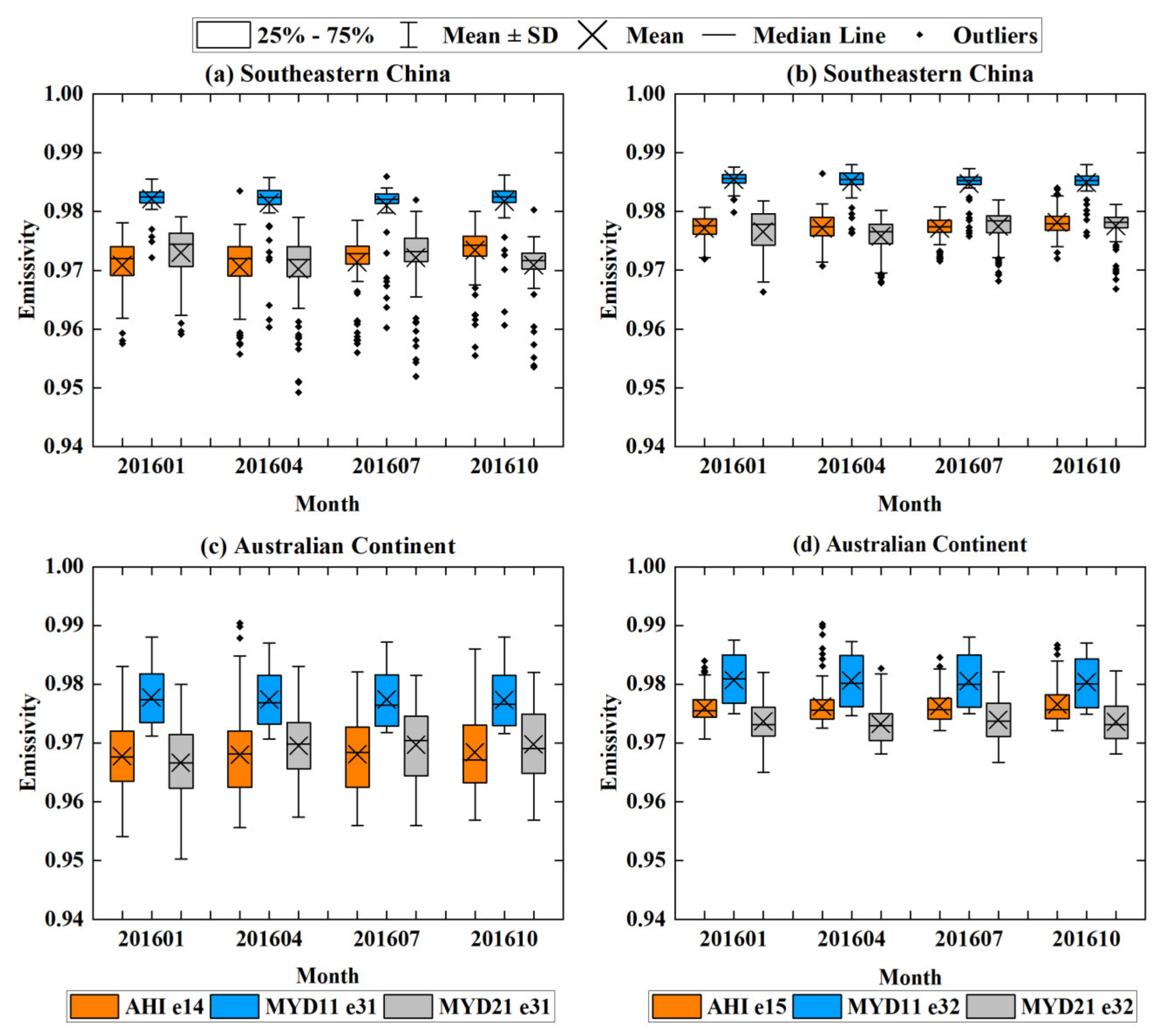
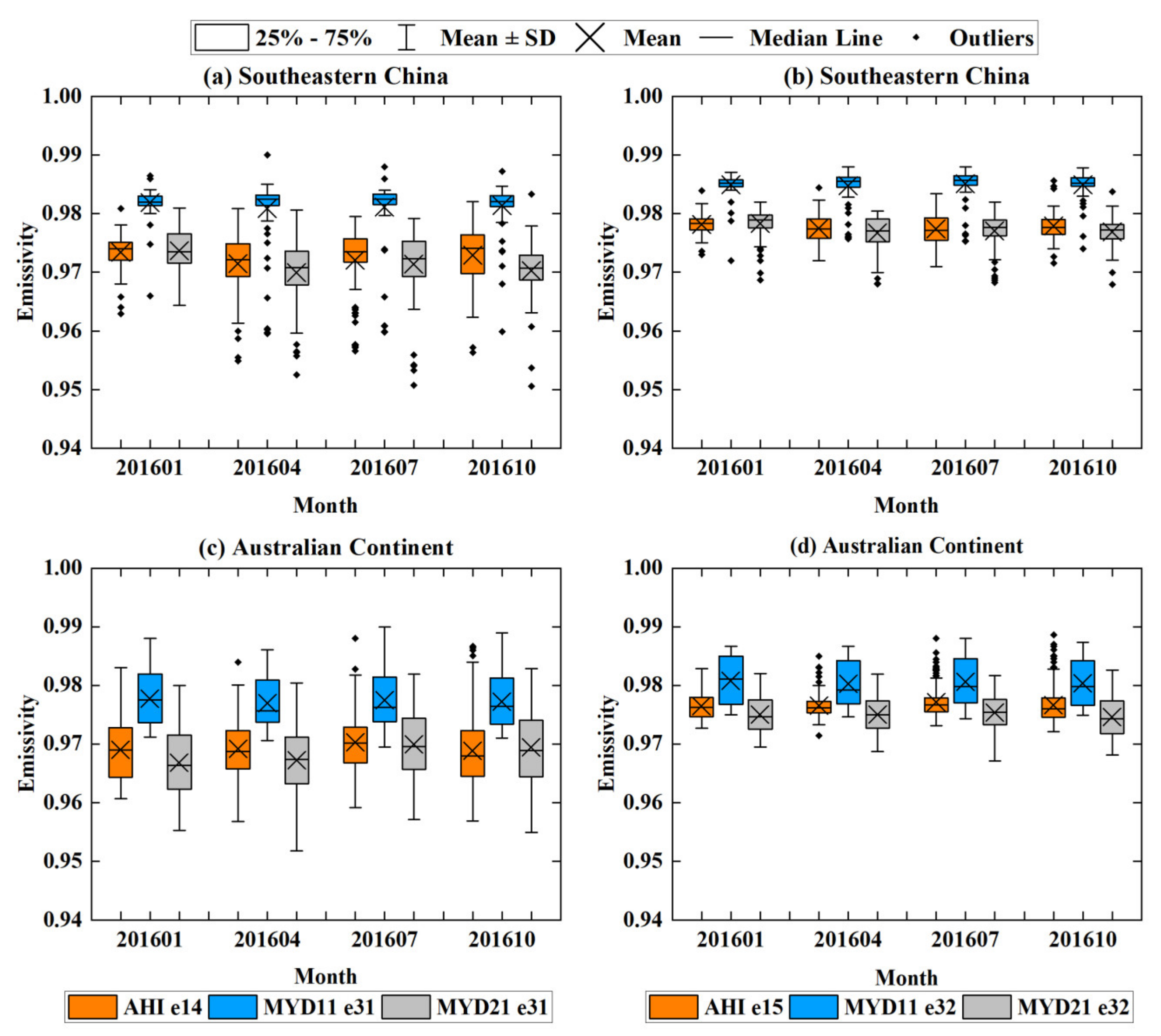
| LSE Products | Daytime | N | Nighttime | N | ||||||||||||
|---|---|---|---|---|---|---|---|---|---|---|---|---|---|---|---|---|
| AHI | MYD11_L2 | MYD21_L2 | AHI | MYD11_L2 | MYD21_L2 | |||||||||||
| Study Area | Season | Month | e14 mean | e14 stdev | e31 mean | e31 stdev | e31 mean | e31 stdev | e14 mean | e14 stdev | e31 mean | e31 stdev | e31 mean | e31 stdev | ||
| Southeastern China | Winter | 201601 | 0.973 | 0.006 | 0.982 | 0.004 | 0.975 | 0.006 | 75,805 | 0.975 | 0.005 | 0.982 | 0.002 | 0.976 | 0.005 | 45,963 |
| Spring | 201604 | 0.973 | 0.006 | 0.982 | 0.003 | 0.972 | 0.006 | 80,997 | 0.973 | 0.007 | 0.982 | 0.004 | 0.972 | 0.007 | 124,586 | |
| Summer | 201607 | 0.974 | 0.006 | 0.982 | 0.004 | 0.971 | 0.006 | 90,589 | 0.973 | 0.006 | 0.982 | 0.004 | 0.971 | 0.007 | 141,554 | |
| Autumn | 201610 | 0.971 | 0.007 | 0.981 | 0.006 | 0.972 | 0.008 | 77,096 | 0.974 | 0.006 | 0.982 | 0.003 | 0.974 | 0.006 | 134,296 | |
| Mean | 0.973 | 0.006 | 0.982 | 0.004 | 0.972 | 0.007 | - | 0.973 | 0.006 | 0.982 | 0.003 | 0.972 | 0.006 | - | ||
| Australian continent | Summer | 201601 | 0.964 | 0.007 | 0.975 | 0.005 | 0.965 | 0.008 | 432,751 | 0.967 | 0.006 | 0.976 | 0.005 | 0.964 | 0.008 | 654,108 |
| Autumn | 201604 | 0.964 | 0.007 | 0.975 | 0.005 | 0.967 | 0.007 | 748,572 | 0.967 | 0.006 | 0.975 | 0.005 | 0.965 | 0.008 | 1,052,311 | |
| Winter | 201607 | 0.964 | 0.007 | 0.975 | 0.005 | 0.966 | 0.008 | 969,707 | 0.968 | 0.006 | 0.976 | 0.005 | 0.967 | 0.009 | 818,831 | |
| Spring | 201610 | 0.964 | 0.007 | 0.974 | 0.004 | 0.967 | 0.008 | 921,616 | 0.967 | 0.006 | 0.975 | 0.005 | 0.967 | 0.008 | 1,176,677 | |
| Mean | 0.964 | 0.007 | 0.975 | 0.005 | 0.966 | 0.008 | - | 0.967 | 0.006 | 0.976 | 0.005 | 0.966 | 0.008 | - | ||
| Sensor | Time Range | Temporal/Spatial Resolution | Algorithm |
|---|---|---|---|
| GOES 13/15 IMAGER | 2009–2018 | 1 h/4 km | dual-window algorithm |
| GOES 16/17 ABI | 2018–2020 | 15 min/2 km | operational SW algorithm |
| MTSAT-2 IMAGER | 2009–2015 | 1 h/4 km | |
| Himawari-8 AHI | 2016–2020 | 10 min/2 km | |
| MSG-2 SEVIRI | 2009–2020 | 15 min/3 km | |
| FY-2E S-VISSR | 2009–2018 | 1 h/5 km | |
| FY-4 AGRI | 2018–2020 | 15 min/4 km |
© 2020 by the authors. Licensee MDPI, Basel, Switzerland. This article is an open access article distributed under the terms and conditions of the Creative Commons Attribution (CC BY) license (http://creativecommons.org/licenses/by/4.0/).
Share and Cite
Li, R.; Li, H.; Sun, L.; Yang, Y.; Hu, T.; Bian, Z.; Cao, B.; Du, Y.; Liu, Q. An Operational Split-Window Algorithm for Retrieving Land Surface Temperature from Geostationary Satellite Data: A Case Study on Himawari-8 AHI Data. Remote Sens. 2020, 12, 2613. https://doi.org/10.3390/rs12162613
Li R, Li H, Sun L, Yang Y, Hu T, Bian Z, Cao B, Du Y, Liu Q. An Operational Split-Window Algorithm for Retrieving Land Surface Temperature from Geostationary Satellite Data: A Case Study on Himawari-8 AHI Data. Remote Sensing. 2020; 12(16):2613. https://doi.org/10.3390/rs12162613
Chicago/Turabian StyleLi, Ruibo, Hua Li, Lin Sun, Yikun Yang, Tian Hu, Zunjian Bian, Biao Cao, Yongming Du, and Qinhuo Liu. 2020. "An Operational Split-Window Algorithm for Retrieving Land Surface Temperature from Geostationary Satellite Data: A Case Study on Himawari-8 AHI Data" Remote Sensing 12, no. 16: 2613. https://doi.org/10.3390/rs12162613
APA StyleLi, R., Li, H., Sun, L., Yang, Y., Hu, T., Bian, Z., Cao, B., Du, Y., & Liu, Q. (2020). An Operational Split-Window Algorithm for Retrieving Land Surface Temperature from Geostationary Satellite Data: A Case Study on Himawari-8 AHI Data. Remote Sensing, 12(16), 2613. https://doi.org/10.3390/rs12162613