Assessment of Leaf Chlorophyll Content Models for Winter Wheat Using Landsat-8 Multispectral Remote Sensing Data

Abstract

The leaf chlorophyll content (LCC) is a critical index to characterize crop growth conditions, photosynthetic capacity, and physiological status. Its dynamic change characteristics are of great significance for monitoring crop growth conditions and understanding the process of material and energy exchange between crops and the environment. Extensive research has focused on LCC retrieval with hyperspectral data onboard various sensor platforms. Nevertheless, limited attention has been paid to LCC inversion from multispectral data, such as the data from Landsat-8, and the potentials and capabilities of the data for crop LCC estimation have not been fully explored. The present study made use of Landsat-8 Operational Land Imager (OLI) imagery and the corresponding field experimental data to evaluate their capabilities and potentials for LCC modeling using four different retrieval methods: vegetation indices (VIs), machine learning regression algorithms (MLRAs), lookup-table (LUT)-based inversion, and hybrid regression approaches. The results showed that the modified triangular vegetation index (MTVI2) exhibited the best estimate accuracy for LCC retrieval with a root mean square error (RMSE) of 5.99 μg/cm² and a relative RMSE (RRMSE) of 10.49%. Several other vegetation indices that were established from red and near-infrared (NIR) bands also exhibited good accuracy. Models established from Gaussian process regression (GPR) achieved the highest accuracy for LCC retrieval (RMSE = 5.50 μg/cm², RRMSE = 9.62%) compared with other MLRAs. Moreover, red and NIR bands outweighed other bands in terms of GPR modelling. LUT-based inversion methods with the “K(x) = −log (x) + x” cost function that belongs to the “minimum contrast estimates” family showed the best estimation results (RMSE = 8.08 μg/cm², RRMSE = 14.14%), and the addition of multiple solution regularization strategies effectively improved the inversion accuracy. For hybrid regression methods, the use of active learning (AL) techniques together with GPR for LCC modelling significantly increased the estimation accuracy, and the combination of entropy query by bagging (EQB) AL and GPR had the best accuracy for LCC estimation (RMSE = 12.43 μg/cm², RRMSE = 21.77%). Overall, our study suggest that Landsat-8 OLI data are suitable for crop LCC retrieval and could provide a basis for LCC estimation with similar multispectral datasets.

1. Introduction

The interaction between global environmental change and terrestrial ecosystems has always been one of the central issues in the study of global change [1]. Vegetation, which covers 70% of the global land area, is an essential indicator of the change of the land ecological environment. It is also the major object of earth observation with remote sensing techniques. The ecological processes related to plant material energy exchange, for instance, photosynthesis, transpiration, respiration, and primary productivity, are in close connection with the biophysical and biochemical parameters of the vegetation. Among these parameters, chlorophyll is a crucial antenna pigment, which is responsible for light absorption and transfer in photosynthesis. Changes in the leaf chlorophyll content (LCC) thus directly affect biochemical processes such as photosynthesis and primary productivity [2]. In agricultural remote sensing research, chlorophyll is also used as an important index of crop growth conditions [3], and its content variations are related to crop stress, the aging process, and nitrogen nutrition [4]. Therefore, quantitative analysis of LCC has important significance, not only for understanding the process of material and energy exchange between plants and the environment, but also for monitoring crop growth, nutritional status, and stress conditions in agricultural applications.

Owning to its remarkable absorption characteristics in the visible range, nondestructive estimation of LCC is possible with spectral analysis and remote sensing techniques, and numerous studies have focused on chlorophyll retrieval methods [5,6,7,8]. Generally, the retrieval approaches can be classified into four methodological categories: parametric regression methods, nonparametric regression methods, physically based model inversion methods, and hybrid regression methods [9], and each method has captured varying degrees of attention in chlorophyll assessment when using multi-spectral or hyperspectral datasets acquired from ground-based, airborne, and space-borne sensors.

Parametric regression methods, such as vegetation indices (VIs), and spectra of first-order and second-order differential characteristics, have been extensively used for chlorophyll retrieval. For example, Pu and Gong [10] compared and analysed the relationship between hyperspectral reflectance, its first-order and second-order differential characteristics, and the leaf chlorophyll content, and it was found that the first-order differential value at 725 nm and the second-order differential value at 705 nm had the highest correlation with LCC, and the values of the correlation coefficients were both higher than 0.7. Based on Medium Resolution Imaging Spectrometer (MERIS) satellite data, Dash and Curran [11] proposed the MERIS terrestrial chlorophyll index (MTCI) using red and red-edge band data, and found that MTCI was suitable for accurate estimation of the crop chlorophyll content. Gitelson et al. [5] established two chlorophyll indices, i.e., green and red-edge chlorophyll indices (CIgreen and CIred-edge), respectively, using a conceptual model, and these two indices showed excellent performance in canopy chlorophyll content retrieval. Yu et al. [4] proposed a ratio of the reflectance difference index (RRDI) based on the multiple scatter correction (MSC) theory. The results indicated that RRDI was accurate for LCC assessment, and it could alleviate the effect of structural characteristics on LCC retrieval to some extent.

Different from parametric methods that use spectral features established from several specific bands, nonparametric methods take advantage of full-spectrum information based on training data to optimize regression algorithms [12]. For instance, Tang et al. [13] investigated and compared multiple linear regression (MLR), back propagation, radial basis function neural networks (BPNN, RBFNN), and partial least squares regression (PLSR) for assessing LCC in soybean plants. Their results suggested that these regression algorithms with wavelet analysis could achieve good estimation results. Among them, RBFNN and PLSR with a Gaussian kernel function showed the best accuracy and stability for LCC retrieval. Zhao et al. [6] utilized three methods, i.e., the Bayesian model average (BMA), PLS, and stepwise multiple regression (SMR), for LCC assessment with abundant measured leaf data. It was found that these three models achieved a good estimation accuracy. Moreover, the BMA algorithm could alleviate the overfitting problem and improve the generalization of the established LCC model compared with PLS and SMR; thus, it was more suitable for LCC retrieval. Based on spaceborne Compact High Resolution Imaging Spectrometer (CHRIS) data and airborne Compact Airborne Spectrographic Imager (CASI) data, Verrelst et al. [14] investigated and tested the Gaussian process regression (GPR) algorithm for LCC estimation. Their results suggested that GPR was suitable for LCC retrieval.

Physically based model inversion was established on the basis of radiative transfer models (RTMs). RTMs are quantitative models that explain the mechanism describing the relationship between spectral reflectance and vegetation biophysical and biochemical parameters. These models can be used to perform abundant simulations based on a robust understanding of physical, chemical, and biological processes [15]. The process with plant input parameters to simulate leaf- or canopy- level reflectance is called ‘forward’, and inversion is the inverse process. Among all RTMs, the leaf optical properties model PROSPECT and canopy bidirectional reflectance model SAIL (Scattering by Arbitrary Inclined Leaves) are widely used in the remote sensing community. Darvishzadeh et al. [16] tested the capability of PROSAIL RTM and ALOS AVNIR-2 multispectral image data using a lookup-table (LUT) approach for assessing the canopy chlorophyll content in paddy rice. Their results demonstrated the ability of the PROSAIL inversion method to estimate the canopy chlorophyll content in paddy rice using ALOS AVNIR-2 multispectral data. For the sake of alleviating the ill-posed issue of LUT-based RTM inversion methods, Rivera et al. [17] analyzed different regularization strategies, including varied cost functions (CFs), applying different levels of noise, and employing multiple best solutions, to relieve the problem of LCC estimation. Their results showed that LUT-based RTM inversion methods together with different regularization strategies evidently improved the estimation accuracy, and employment of a normalized “L1-estimate” CF in the inversion process achieved the best estimation with a relative error of 17.6%. Zhang and Wang [18] conducted research on the assessment of LCC in Tamarix ramosissima via inversion of PROSPECT RTM by introducing a merit function. They used its calibrated version instead of the original PROSPECT-4 and found that the calibrated PROSPECT-4 was more accurate for the retrieval of LCC with a root mean square error (RMSE) value of 28.79 mg/m². Croft et al. [19] evaluated the capability of LUT-based RTM inversion methods for LCC assessment with multi-spectral Landsat-8 imagery. They adopted a two-step inversion process using coupled PROSPECT and SAIL RTMs, and it exhibited an accurate estimation (RMSE = 16.18 μg/cm²) of LCC with Landsat-8 data.

Hybrid regression methods take advantage of both physically based techniques and machine learning regression algorithms (MLRAs). That is, these approaches utilize abundant synthetic data simulated by RTMs instead of measured data collected from field campaigns for training machine learning regression models, so as to improve the generalization and computational efficiency of the models. For instance, Malenovsky et al. [8] investigated the combination of continuum removal and RTM for LCC retrieval from the data acquired by Airborne Imaging Spectroradiometer (AISA) Eagle. They applied a continuum removal technique to PROSPECT-DART (discrete anisotropic radiative transfer) simulations and then used these data to train an artificial neural network (ANN). Their ground validation results showed that the ANN and PROSPECT-DART hybrid approach was accurate for LCC estimation, with an RMSE value of 2.18 μg/cm² and a relative RMSE (RRMSE) value of 4.18%. To mitigate the problem of computational costs for MLRAs, especially when the amount of RTMs training data is extremely large, Verrelst et al. [20] employed active learning (AL) techniques so as to optimize sample selection from simulated Sentinel-3 Ocean and Land Color Instrument (OCLI) data for training Kernel-based MLRAs. Their results suggested that AL methods were more efficient than random sampling in choosing appropriate samples for training the MLRAs, since MLRAs together with AL techniques exhibited better estimation accuracy than the results with random sampling. Research conducted by Upreti et al. [21] for LCC retrieval with Sentinel-2 data also supported the conclusion that the AL technique was efficient in selecting samples for training MLRAs.

The above-mentioned literature has indeed enriched the methodologies for LCC assessment with remote sensing techniques. Nevertheless, each retrieval method had its own drawbacks that need to be avoided or overcome. For parametric regression methods, the representativeness of experimental samples and the physical mechanism of remote sensing models are crucial to the effectiveness and universality of these models. However, the problem of overfitting training data collected from field experiments may be incurred by flexible model definitions when nonparametric methods are used. In order to mitigate this overfitting issue, various advanced machine learning algorithms had been considered for LCC retrieval [12]. In terms of RTM inversion, the inversion process is actually an ill-posed problem, since different combinations of leaf-level and canopy-level parameters could lead to very similar simulations of canopy reflectance. Moreover, simplifications and idealization of some processes in RTMs could produce inaccuracies for canopy reflectance modeling [22]. LUT-based RTM inversion strategies and different regularization strategies might be efficient to mitigate the ill-posed issue, and to better handle the inversion process. For hybrid regression methods, it should be noted that these approaches do not alleviate the main issues of RTMs; they merely use all available data simulated by RTMs to train machine learning regression models. Nevertheless, the main shortcoming of these models with respect to adopting hybrid methods is the computation cost. AL approaches, which are intended for selection of optimal samples from a training data pool, can be promising for obtaining an optimized training set and increasing computational efficiency for hybrid methods. Thus, optimizing and improving different LCC retrieval methods are needed, particularly for the application of these methods to various new sensors for LCC estimation.

In recent years, with the rapid advance of earth observation technologies, newly launched satellite sensors, such as the Gaofen (GF) series in China, Sentinel series in Europe, and Landsat-8 in the US, offer huge potential for enrichment of LCC retrieval methodologies. The Landsat-8 Operational Land Imager (OLI) is the newest senor by far in the Landsat observation project. Compared to previous sensors, the Landsat-8 OLI sensor has advanced spectral bands and radiometric resolution, a better signal-to-noise ratio, and it has been used for various purposes in the terrestrial ecosystem [23]. Nevertheless, limited studies have reported an investigation of Landsat-8 OLI data or Landsat series datasets for plant LCC retrieval [19,24,25]. Research on the potential and capability of LCC modelling using Landsat-8 OLI data has a profound influence: on the one hand, robust and accurate LCC models from different satellite sensors could be used together for deriving high-frequency LCC products for rapid monitoring of agricultural crops; on the other hand, these models could provide methods and technical support for applications of similar multispectral sensors onboard unmanned aerial vehicles (UAVs) for LCC estimation at a specific fine scale. Therefore, the aim of the present study was to assess the capability of Landsat-8 OLI data for LCC modelling with different retrieval methods. The specific objectives were to: (i) investigate the performance of broadband vegetation indices in LCC assessment with Landsat-8 OLI data; (ii) inspect the ability of machine learning regression algorithms in LCC retrieval; (iii) establish LUT-based RTM inversion based on Landsat-8 OLI data using different regularization strategies to optimize LCC estimation; and iv) explore the feasibility of hybrid methods using computationally demanding MLRAs with different active learning strategies for LCC retrieval.

2. Materials and Methods

2.1. Field Experiments

Field experiments were conducted in Shunyi District (40°08′N, 116°39′E), Beijing, China (Figure 1) during the 2016 growing season. The area has a warm temperate climate, with mean annual rainfall of 620.0 mm, a mean annual temperature of 11.2 °C, and it is mainly characterized by fluvo-aquic soil. The average topsoil nutrient status of the region (0–0.30 m depth) was as follows: organic matter 14.23 g/kg, total nitrogen 0.90 g/kg, available phosphorus 30.63 mg/kg, and rapidly available potassium 123.75 mg/kg. In 2015, three major cultivars of winter wheat (Nongda 212, Zhongmai 12, and Nongda 5181) were planted in this district during the period from 25 September to 5 October. Fertilization and irrigation were applied according to local standard practice managed by farmers. In the 2016 campaigns, twenty-four elementary sampling units (ESUs), in which a single cultivar had been planted, were established in farmers’ fields. The size of the ESUs was approximately 30 m × 30 m, corresponding to the spatial resolution of Landsat-8 imagery, and the locations were within the fields and far from the field borders. Four field surveys at different growth stages, whose dates were close to Landsat-8 acquisitions, were conducted during the whole growing period of winter wheat. Detailed information on the experiment is listed in

Table 1. Summary of Landsat-8 acquisitions and field data collection dates, as well as the statistics of the leaf chlorophyll content of winter wheat.

Field Data Collection Date	Growth Stage	Imagery Date	ESUs	Leaf Chlorophyll Content (μg·cm−2) a
				AVG	MAX	MIN
2016/04/20	Booting	2016/04/18	24	54.33	66.77	28.06
2016/05/03	Heading	2016/05/04	24	59.89	77.65	29.78
2016/05/18	Flowering	2016/05/20	24	61.64	78.98	41.59
2016/06/07	Milking	2016/06/05	24	47.78	64.49	18.33

^a Leaf chlorophyll contents were converted from SPAD readings using the relationship proposed by Cerovic et al. [26].

.

2.2. Ground Data Measurements

On each sampling date, chlorophyll readings of winter wheat were made in five homogeneous crop areas (each in a 1 m × 1 m area) randomly distributed inside each ESU using a SPAD-502 (Konica-Minolta, Tokyo, Japan). Measurements were performed on the top-most leaves of different wheat plants per area, and a total of 50 measurements were taken to obtain a mean value of chlorophyll SPAD reading per ESU. These SPAD readings were converted to the leaf chlorophyll content (mass per unit leaf area, μg·cm⁻²) using the relationship “LCC = (99SPAD)/(144-SPAD)” proposed by Cerovic et al. [26], which achieved a conversion accuracy of approximately 4 μg·cm⁻² for monocot (wheat and maize) species. Apart from chlorophyll SPAD measurements, the central position of each ESU was geo-located with GPS measurements for subsequently associating the leaf chlorophyll content estimation with the corresponding Landsat-8 OLI multispectral data.

2.3. Landsat-8 Imagery Processing

Landsat-8 OLI images, which were close to the dates of field experiments, were firstly downloaded from Earth Explorer (https://earthexplorer.usgs.gov/). These downloaded images were then preprocessed through radiometric calibration and atmospheric correction to obtain surface reflectance data using radiometric calibration and Fast Line-of-sight Atmospheric Analysis of Spectral Hypercubes (FLAASH) processing tools in ENVI 5.1 software (Exelis Visual Information Solutions, Boulder, CO, USA, 2014). For the sake of concentrating on the winter wheat area, processed Landsat-8 imagery was clipped to a 1483 × 1121 pixel size using the boundary of Shunyi district, and then multi-band spectral data of the ESUs were extracted from the clipped images. Nevertheless, owning to slight cloud contamination of the images acquired on the dates of 18 April, 20 May, and 5 June, a total of 3, 2, and 5 ESUs that were contaminated by cloud in these images were not included. Finally, a total of 86 ESUs with corresponding Landsat-8 multi-band spectral data and leaf chlorophyll contents was considered for subsequent modelling and analysis.

2.4. PROSAIL Simulated Dataset

Leaf-level RTM PROSPECT-5 [15] coupled with the canopy bidirectional reflectance model 4SAIL [27], which is referred to as the PROSAIL model, was used for the generation of a simulated dataset in the present study. PROSPECT-5 simulates leaf directional-hemispherical reflectance and transmittance from 400 to 2500 nm with six input variables: leaf chlorophyll content (LChl), leaf carotenoid content (LCar), leaf structure parameter (N), leaf mass per area (LMA), equivalent water thickness (EWT), and brown pigments (Cbrown), while parameters such as the leaf area index (LAI), leaf angle distribution (LAD), hot-spot parameter (hots), fraction of diffuse incoming solar radiation (skyl), sun zenith angle (θs), view zenith angle (θv), relative azimuth angle (ϕ), leaf directional-hemispherical reflectance and transmittance derived from PROSPECT-5, and reflectance spectrum of moist and dry soil are needed for 4SAIL to output canopy bidirectional reflectance. Here, LAD was characterized by the average leaf angle (ALA), and ALA was illustrated by an ellipsoidal distribution [28]. Reflectance of moist and dry soil was measured during the field experiments with an ASD FieldSpec 3 spectrometer (Analytical Spectral Devices, Inc., Boulder, CO, USA). Moreover, a scaling factor (α_soil) was employed in 4SAIL so as to consider soil brightness variations as a function of these two soil types [14].

Table 2. Statistics of the input variables of the PROSPECT-5 and 4SAIL models used to generate the training dataset.

Model Parameter		Units	Range	Distribution a	Number
PROSPECT-5	Leaf structure index (N)	unitless	1.0–1.8	Gaussian (μ: 1.4, SD: 0.5)	3
	Leaf chlorophyll content (LChl)	[μg/cm2]	10–100	Gaussian (μ: 50, SD: 30)	50
	Leaf carotenoid content (LCar)	[μg/cm2]	12		1
	Leaf dry matter content (Cm)	[g/cm2]	0.001–0.01	Gaussian (μ: 0.005, SD: 0.005)	3
	Leaf water content (Cw)	[cm]	0.01		1
	Brown pigments (Cbp)	unitless	0		1
4SAIL	Leaf area index (LAI)	[m2/m2]	0–10	Gaussian (μ: 3, SD: 4)	10
	Average leaf angle (ALA)	[°]	40–70	Gaussian (μ: 55, SD: 10)	3
	Soil scaling factor (αsoil)	unitless	0–1	Gaussian (μ: 0.5, SD: 0.3)	3
	Hot spot parameter (hots)	unitless	0.1–0.5	Gaussian (μ: 0.2, SD: 0.5)	3
	Fraction of diffuse incoming solar radiation (skyl)	unitless	10		1
	Sun zenith angle (θS)	[°]	30		1
	View zenith angle (θV)	[°]	8		1
	Sun-sensor azimuth angle (Φ)	[°]	135		1

^a μ refers to the mean value, SD is the standard deviation.

presents the ranges, statistical distribution, and number of classes of the input parameters for PROSAIL model simulation. These parameters statistics were based on values measured during field campaigns and other existing studies [21]. Gaussian input distributions were used for N, LChl, Cm, LAI, ALA, α_soil, and hots to fit the actual distribution of these parameters for winter wheat during the growing stages. Sun and viewing conditions were set to the same situation as the Landsat-8 satellite overpass.

In total, 121,500 simulated canopy bidirectional reflectance data points were produced by performing PROSAIL using a random combination of all the input parameters. Then, the simulated data were resampled, using Landsat-8 spectral response functions, to six bands, i.e., blue, green, red, near-infrared (NIR), short-wave infrared 1 (SWIR 1), and short-wave infrared 2 (SWIR 2) bands, (Coastal, Pan, and Cirrus bands were excluded). Since differences might exist between simulated and actual Landsat-8 data, Gaussian noise was added to the simulated data so as to better describe the actual Landsat-8 characteristics. The equation for computing the Gaussian noise was as follows [29]:

R^*(λ) = R(λ)(1 +MD(λ) + MI)/100) + AD(λ) + AI

(1)

where R^*(λ) and R(λ) are the processed Landsat-8 reflectance with noise and the unprocessed simulated reflectance data, respectively. MD and MI are the multiplicative wavelength dependent noise and multiplicative wavelength independent noise, respectively. Similarly, AD and AI are the additive wavelength dependent noise and independent noise, respectively. Referring to Weiss and Baret [29] and Upreti et al. [21], A value of 0.01 was used for AD and AI, and values of MD and MI were set as 2% and 1%, respectively, for all ands.

2.5. Chlorophyll Modelling Methods

To evaluate the capability of Landsat-8 OLI data for chlorophyll assessment, different retrieval methods, including vegetation indices (VIs), machine learning regression algorithms (MLRAs), lookup -table (LUT)-based inversion, and hybrid regression, were used. The methodology adopted in this work is shown in Figure 2.

2.5.1. Vegetation Indices

Since the available bands of the Landsat-8 OLI sensor were blue, green, red, NIR, SWIR 1, and SWIR 2 bands, VIs composed by blue, green, red, and NIR bands were considered for evaluation of Landsat-8 OLI imagery for chlorophyll modelling. The selected VIs included the normalized difference vegetation index (NDVI), green normalized difference vegetation index (GNDVI), simple ratio (SR), modified simple ratio (MSR), enhanced vegetation index (EVI), enhanced vegetation index 2 (EVI2), optimized soil adjusted vegetation index (OSAVI), modified soil adjusted vegetation index (MSAVI), and modified triangular vegetation index (MTVI2). Detailed information on these VIs is listed in

Table 3. Spectral indices used in this study.

Spectral Index	Formula a	Reference
Normalized difference vegetation index (NDVI)	$(R_{NIR}-R_{Red})/(R_{NIR}+R_{Red})$	[30]
Green normalized difference vegetation index (GNDVI)	$(R_{NIR}-R_{Green})/(R_{NIR}+R_{Green})$	[31]
Simple ratio (SR)	$R_{NIR}/R_{Red}$	[32]
Modified simple ratio (MSR)	$\left(R_{NIR}/R_{Red}-1\right)/\sqrt{R_{NIR}/R_{Red}+1}$	[33]
Enhanced vegetation index (EVI)	$\hspace{1em}2.5\times (R_{NIR}-R_{Red})/(R_{NIR}+6.0\times R_{Red}-7.5\times R_{Blue}+1)$	[34]
Enhanced vegetation index 2 (EVI2)	$2.5\times (R_{NIR}-R_{Red})/(R_{NIR}+2.4\times R_{Red}+1)$	[35]
Optimized soil adjusted vegetation index (OSAVI)	$\left(1+0.16\right)(R_{NIR}-R_{Red})/(R_{NIR}+R_{Red}+0.16)$	[36]
Modified soil adjusted vegetation index (MSAVI)	$(2\times R_{NIR}+1-\sqrt{{\left(2\times R_{NIR}+1\right)}^2-8\times (R_{NIR}-R_{Red})})/2$	[37]
Modified triangular vegetation index (MTVI2)	$$\begin{gathered} \hspace{1em}1.5\times (1.2\times (R_{NIR}-R_{Green})-2.5\times \left(R_{Red}-R_{Green}\right))/ \\ \hspace{1em}\sqrt{{\left(2\times R_{NIR}+1\right)}^2-\left(6\times R_{NIR}-5\times \sqrt{R_{Red}}\right)-0.5} \end{gathered}$$	[38]

^a R_λ is the reflectance value at band λ (nm).

.

2.5.2. Machine Learning Regression Algorithms

MLRAs, which capture nonlinear relationships between the input (e.g., band reflectance features) and output (e.g., biochemical parameters) through training flexible modes with input datasets, are effective approaches for agronomy parameter retrieval. Here, six MLRAs were selected on consideration of their fast training, good performance, and popularity in various application domains for the purpose of investigation and evaluation of Landsat-8 OLI data for leaf chlorophyll content modelling. These six MLRAs were partial least square regression (PLSR), random forest (RF), feedforward neural networks (FNN), support vector regression (SVR), kernel ridge regression (KRR), and Gaussian processes regression (GPR). Six reflectance bands, i.e., blue, green, red, NIR, SWIR 1, and SWIR 2 bands, were used as input features for these MLRAs. Here, PLSR was optimized using a leave-one-out cross-validation (LOOCV) scheme to determine the number of latent variables by minimizing the predicted residual sums of squares (PRESS). As for the RF algorithm, the number of regression trees and the numerical value of a random subset of variables were optimized based on a k-fold cross-validation scheme. For FNN optimization, the Levenberg-Marquardt learning algorithm with a squared loss function was selected, and a k-fold cross-validation procedure was used to avoid overfitting problems. Initial weights of the FNN model were generated by the Nguyen-Widrow method, and model regularization was conducted by limiting the maximum number of net weights to half the number of training samples. For the implementation of SVR and KRR, a radial basis function (RBF) kernel was used for these two algorithms, regularization parameter, tolerance value, and a kernel parameter were used for SVR, and regularization and kernel parameters for KRR were optimized with a k-fold cross-validation strategy. Regarding the GPR model, a scaled Gaussian kernel function was selected, and model hyperparameters and weights were optimized by maximizing the marginal likelihood in the training data. A list of brief introductions on these methods is presented in

Table 4. Summary of the MLRA algorithms investigated in this study.

Methods	Brief Description	Reference
Partial least square regression (PLSR)	PLSR combines principal component analysis with canonical correlation analysis, which could overcome the problem of multicollinearity between traditional independent variables, and the extracted PLS factors could explain most of the variation in both the predictors and response variables.	[39]
Random forest (RF)	RF regression is a fusion algorithm based on a decision tree classifier, which uses a bootstrap resampling method to extract multiple samples, and decision trees are constructed for each sample; then, the predicted average values of all decision trees are taken as the final prediction results.	[40]
Feedforward neural networks (FNN)	Neural networks (NN) refer to a complex network structure formed by the interconnection of a large number of processing units (neurons). Here, the standard multi-layer FNN model was adopted, and the Levenberg-Marquardt learning algorithm with a squared loss function was selected to optimize the established NN structure.	[41]
Support vector regression (SVR)	SVR maps training samples to a high-dimensional space and transforms a nonlinear problem in low-dimensional space to a linear problem in high-dimensional space, and then carries on linear modeling. Here, a radial basis function was used to transform nonlinear problems to linear ones.	[42]
Kernel ridge regression (KRR)	KRR is a regression algorithm based on the kernel method. It uses a kernel function to map original data to a high-dimensional space. The mapped data show a linear relationship in the high-dimensional space, and the established model has a strong generalization ability.	[43]
Gaussian processes regression (GPR)	GPR is a statistical learning method under the Bayesian framework, which is often used in nonlinear modeling. It can transform a prior distribution into a posterior model by training historical data, so as to obtain prediction results with probability significance.	[44]

.

2.5.3. LUT-Based Inversion Strategies

LUT-based inversion strategies are extensively-used solutions in physically-based model inversion methodologies, which identify a synthetic reflectance set that is most similar to an actual one, by inquiring the LUT generated from RTMs, applying a cost function, and setting various regularization strategies. A cost function is used to minimize the difference between simulated and measured data for all wavebands [12], while regularization strategies are aimed at alleviating the ill-posed problem, and to better handle the inversion process. In the present study, ten cost functions (CFs) that belong to three different families (“information measures”, “M-estimates”, and “minimum contrast estimates”) were investigated and compared. Detailed information on these ten CFs is listed in

Table 5. Cost functions used in the present study.

Category	Cost Function	Algorithm a
Information measures	Pearson chi-square	$D\left[P,Q\right]={{\displaystyle \sum }}_{{\lambda }_l=1}^{{\lambda }_n}\frac{{\left(q\left({\lambda }_l\right)-p\left({\lambda }_l\right)\right)}^2}{p\left({\lambda }_l\right)}$
	K-divergence Lin	$D\left[P,Q\right]={{\displaystyle \sum }}_{{\lambda }_l=1}^{{\lambda }_n}p\left({\lambda }_l\right)\ln \left(\frac{2p\left({\lambda }_l\right)}{p\left({\lambda }_l\right)+q\left({\lambda }_l\right)}\right)$
	Negative exponential disparity	$D\left[P,Q\right]={{\displaystyle \sum }}_{{\lambda }_l=1}^{{\lambda }_n}q\left({\lambda }_l\right)\left(exp\left(-\frac{p\left({\lambda }_l\right)-q\left({\lambda }_l\right)}{q\left({\lambda }_l\right)}\right)-1\right)$
	Jeffreys-Kullback-Leibler	$D\left[P,Q\right]={{\displaystyle \sum }}_{{\lambda }_l=1}^{{\lambda }_n}\left(p\left({\lambda }_l\right)-q\left({\lambda }_l\right)\right)\left(\ln \left(p\left({\lambda }_l\right)\right)-\ln \left(q\left({\lambda }_l\right)\right)\right)$
M-estimates	Root mean square error	$D\left[P,Q\right]=\sqrt{\frac{{\sum }_{{\lambda }_l=1}^{{\lambda }_n}{\left(p\left({\lambda }_l\right)-q\left({\lambda }_l\right)\right)}^2}{n}}$
	Least absolute error	$D\left[P,Q\right]={{\displaystyle \sum }}_{{\lambda }_l=1}^{{\lambda }_n}\left|p\left({\lambda }_l\right)-q\left({\lambda }_l\right)\right|$
	Geman and McClure	$D\left[P,Q\right]={{\displaystyle \sum }}_{{\lambda }_l=1}^{{\lambda }_n}\frac{{\left(p\left({\lambda }_l\right)-q\left({\lambda }_l\right)\right)}^2}{(1+{\left(p\left({\lambda }_l\right)-q\left({\lambda }_l\right)\right)}^2)}$
Minimum contrast estimates	K(x) = -log (x) + x	$D\left[P,Q\right]={{\displaystyle \sum }}_{{\lambda }_l=1}^{{\lambda }_n}\left\{-\log \left(\frac{q\left({\lambda }_l\right)}{p\left({\lambda }_l\right)}\right)+\frac{q\left({\lambda }_l\right)}{p\left({\lambda }_l\right)}\right\}-1$
	K(x) = log (x) + 1/x	$D\left[P,Q\right]={{\displaystyle \sum }}_{{\lambda }_l=1}^{{\lambda }_n}\left\{\log \left(\frac{q\left({\lambda }_l\right)}{p\left({\lambda }_l\right)}\right)+\frac{q\left({\lambda }_l\right)}{p\left({\lambda }_l\right)}\right\}-1$
	K(x) = log (x)2	$D\left[P,Q\right]={{\displaystyle \sum }}_{{\lambda }_l=1}^{{\lambda }_n}{\left\{\log \left(q\left({\lambda }_l\right)\right)-\log \left(p\left({\lambda }_l\right)\right)\right\}}^2$

^a D[P, Q] represents the distance between two functions, where P = (p(λ₁), …, p(λ_n)) is the multispectral reflectance derived from Landsat-8 OLI satellite data and Q = (q(λ₁), …, q(λ_n)) is the LUT containing simulated Landsat-8 OLI multispectral reflectances with λ₁, …, λ_n representing n spectral bands. Here, the value of n is 6.

. In addition, two regularization strategies were used: the adding of Gaussian noise to the simulated canopy reflectance (Section 2.4), and a range from 0 (single best solution) to the mean of the 30% best solutions at an increment of 2% was included.

2.5.4. Hybrid Regression Methods

Different from MLRAs and LUT-based inversion, hybrid regression approaches use simulated data generated by RTMs and stored in LUTs for training machine learning regression models instead of ground collected data. Nevertheless, the training process of machine learning regression models might be the computational cost when the amount of used RTM-simulated data increases. For the sake of computational efficiency, we investigated and tested six AL methods that belong to two different families (uncertainty and diversity), with a kernel-based MLRA (i.e., GPR) for the capability of hybrid regression methods in LCC modelling using Landsat-8 OLI data. These AL techniques were variance-based pool of regressors (PAL), entropy query by bagging (EQB), residual regression AL (RSAL), angle-based diversity (ABD), Euclidean distance-based diversity (EBD), and cluster-based diversity (CBD). For details on these six AL approaches, refer to Verrelst et al. [20]. For AL implementation, ten subsets each with a number of 2500 were randomly selected from the simulation in Section 2.4 as learning datasets. A random subset of 50 samples was firstly chosen from one learning dataset as initial training data for model training by GPR. Then, samples from the remaining learning dataset (2450 samples) were added to the preliminary training data (50 samples per iteration) using six different AL techniques, with a stopping criteria of 100 iterations or an RMSE decrease lower than 50%. This process was repeated 10 times with different learning datasets. In comparison, the full subset of 2500 samples was trained using GPR without ALs as a reference.

2.6. Statistical Analysis

For VI methods, linear regression models were adopted for establishing relationships between LCC and VIs derived from Landsat-8 OLI data. A k-fold (k = 10) cross-validation procedure and the same k-fold partitions were used for both VI methods and MLRAs. The performance of the VI methods and MLRAs was evaluated by examining the cross-validation estimation of RMSE and RRMSE. For LUT-based inversion strategies and hybrid regression methods, experimental measured data (n = 86) were used for ground validation with RMSE and RRMSE. The implementation of LUT-based inversion and hybrid regression was performed using the Automated Radiative Transfer Models Operator (ARTMO) Toolbox version 3.26 [9] within Matlab software.

3. Results

3.1. LCC Estimation with VIs

The calibration results for LCC assessment with VIs are reported in

Table 6. Calibration results of VIs for LCC assessment.

Index	Equation	R2	RMSE (μg·cm−2)	RRMSE (%)
NDVI	y = 48.61x + 28.16	0.42 **	6.61	11.58
GNDVI	y = 37.01x + 35.92	0.28 **	7.39	12.95
SR	y = 3.53x + 41.79	0.34 **	7.09	12.41
MSR	y = 12.21x + 40.02	0.38 **	6.87	12.04
EVI	y = 41.83x + 33.78	0.37 **	6.91	12.10
EVI2	y = 66.55x + 28.04	0.52 **	6.02	10.54
OSAVI	y = 61.50x + 25.52	0.49 **	6.23	10.90
MSAVI	y = 67.65x + 28.51	0.52 **	6.01	10.53
MTVI2	y = 70.62x + 29.87	0.55 **	5.82	10.19

Note: x and y in the Equation column refer to VIs and LCC, respectively. ** indicates statistical significance at 0.01.

. The performance of different VIs for LCC modelling varied. NDVI exhibited an acceptable relationship with LCC, with an R² value of 0.42, an RMSE of 6.61 μg/cm², and an, RRMSE of 11.58%. In comparison, the ability of GNDVI to assess LCC was rather poor (R² = 0.28, RMSE = 7.39 μg/cm², RRMSE = 12.95%). SR showed a poor relationship with LCC, with a R² value of 0.34, an RMSE of 7.09 μg/cm², and an RRMSE of 12.41%. As for MSR, its relationship with LCC was slightly improved (R² = 0.38, RMSE = 6.87 μg/cm², RRMSE = 12.04%). Compared with the performance of EVI (R² = 0.37, RMSE = 6.91 μg/cm², RRMSE = 12.10%), EVI2 behaved much better in estimating LCC, with an R² value of 0.52, an RMSE of 6.02 μg/cm², and an RRMSE of 10.54%. OSAVI and MSAVI exhibited good relationships with LCC, but MSAVI performed slightly better (R² = 0.52, RMSE = 6.01 μg/cm², RRMSE = 10.53%). Among all VIs, MTVI2 exhibited the best relationship with LCC, with an R² value of 0.55, an RMSE of 5.82 μg/cm², and an RRMSE of 10.19%.

The cross-validation results of these VIs for LCC estimation are presented in Figure 3. The performances of all VIs during cross validation showed a good consistency with their behavior in the calibration process. MTVI2 showed the best estimation accuracy of LCC, with an R² value of 0.53, an RMSE of 5.99 μg/cm², and an RRMSE of 10.49%. The fitted line between the measured and predicted LCC was the closest to the 1:1 line among all VIs. MSAVI, EVI2, and OSAVI exhibited satisfactory estimation results of LCC (R² > 0.4, RMSE < 6.5 μg/cm², RRMSE < 11.3%). Among them, MSAVI and EVI2 showed a very similar prediction accuracy, which accorded with their behavior in the calibration results. NDVI, EVI, and MSR showed acceptable results in LCC estimation with R² around 0.35, and RMSE and RRMSE approximated 7.0 μg/cm² and 12%, respectively. SR and GNDVI showed the worst estimation of LCC with R² lower than 0.30, RMSE higher than 7.2 μg/cm², and RRMSE higher than 12.7%. Although the estimation accuracy differed among selected VIs, it was obvious that all these VIs had obvious insensitivity to low LCC values (< 30 μg/cm²). Furthermore, two sample points with LCC values of approximated 80 μg/cm² were evidently underestimated by all VIs.

3.2. MLRAs in LCC Assessment

The performance of different MLRAs in LCC estimation is shown in Figure 4. Overall, these MLRAs exhibited good estimation results compared with VI methods. PLSR, RF, FNN, and SVR showed a similar estimation accuracy; SVR performed slightly better (R² = 0.50, RMSE = 6.16 μg/cm², RRMSE = 10.80%). Among them, the fitted line between measured and predicted LCC produced by FNN was the closest to the 1:1 line. Compared with these four MLRAs, KRR behaved even better with an R² value of 0.54, an RMSE of 5.94 μg/cm², and an RRMSE of 10.39%. Moreover, the slope of its fitted line between measured and predicted LCC was nearer to 1, and the intercept value was closer to 0. Among all MLRAs, GPR showed the most accurate results for LCC estimation (R² = 0.60, RMSE = 5.50 μg/cm², RRMSE = 9.62%). Furthermore, it showed more sensitivity to LCC values lower than 40 μg/cm² compared to other MLRAs. However, similar to VI methods, two sample points with LCC values close to 80 μg/cm² were also underestimated by all MLRAs.

3.3. LUT-Based Inversion for LCC Estimation

Since the mean of multiple best solutions that ranged from 0 to 30% at an increment of 2% was used for all selected CFs, only the top ten ranked ground validation results of LUT-based inversion for LCC retrieval are reported in

Table 7. Ground validation results of LUT-based inversion with Landsat-8 OLI data.

Cost Function	Rank	RMSE (μg·cm−2)	RRMSE (%)	Mult. Sol. (%)
Pearson chi-square	2	8.94	15.65	8
K-divergence Lin	7	16.15	28.29	30
Negative exponential disparity	10	18.54	32.48	30
Jeffreys-Kullback-Leibler	8	16.47	28.84	30
Root mean square error	9	17.75	31.08	30
Least absolute error	4	11.70	20.49	30
Geman and McClure	3	10.20	17.86	30
K(x) = −log (x) + x	1	8.08	14.14	4
K(x) = log (x) + 1/x	6	13.32	23.33	30
K(x) = log (x)2	5	12.99	22.75	12

. For different CFs, their performance varied markedly. “Pearson chi-square” CF with 8% multiple solutions had the best estimation results (RMSE = 8.94 μg/cm², RRMSE = 15.65%), while “Negative exponential disparity” CF (30% multiple solutions) showed the worst results with an RMSE of 18.54 μg/cm² and an RRMSE of 32.48% among the “information measures” category. “K-divergence Lin” and “Jeffreys-Kullback-Leibler” CFs exhibited similar estimation results with RMSE close to 16 μg/cm², and RRMSE approximated 28%. For CFs among the “M-estimates” type, “Geman and McClure” with 30% multiple solutions had slightly better results (RMSE = 10.20 μg/cm², RRMSE = 17.86%) than those of the “Least absolute error”. In comparison, “root mean square error” CF with 30% multiple solutions showed rather poor results, with an RMSE of 17.75 μg/cm² and an RRMSE of 31.08%. The “K(x) = −log (x) + x” CF, which belongs to the “minimum contrast estimates” family with 4% multiple solutions, showed the best estimation accuracy (RMSE = 8.08 μg/cm², RRMSE = 14.14%) among all the selected 10 CFs. By contrast, the other two CFs from “minimum contrast estimates”, i.e., “K(x) = log (x) + 1/x” and “K(x) = log (x)²”, showed slightly inferior estimates with values of RMSE and RRMSE close to 13 μg/cm² and 23%, respectively.

3.4. Hybrid Regression Methods in LCC Modelling

The results of GPR with different AL methods for LCC retrieval are presented in

Table 8. Validation results of hybrid regression methods with Landsat-8 OLI data.

Method	Cross-Validation		Ground-Validation
	RMSE (μg·cm−2)	RRMSE (%)	RMSE (μg·cm−2)	RRMSE (%)
GPR + CBD	13.83	24.60	14.53	25.44
GPR + EBD	14.59	25.87	14.46	25.33
GPR + ABD	15.19	26.92	16.44	28.78
GPR + PAL	14.73	26.12	14.13	24.74
GPR + EQB	17.02	30.17	12.43	21.77
GPR + RSAL	14.75	26.15	13.17	23.06
GPR	16.93	30.00	31.98	56.00

. The GPR approach for LCC estimation is also included for comparison. For AL approaches that belong to the diverse family, GPR with CBD behaved the best in the cross-validation process, with an RMSE of 13.83 μg/cm² and an RRMSE of 24.60%, while GPR with EBD showed the best results in the ground-validation process (RMSE = 14.46 μg/cm², RRMSE = 25.33%). By contrast, GPR with ABD exhibited inferior estimations for both the cross-validation and ground-validation processes. Different from the results of diverse ALs, the estimation results of GPR with uncertainty ALs (i.e., PAL, EQB, and RSAL) in the ground validation were better than those in the cross validation. Furthermore, the ground-validation estimation results from uncertainty ALs were slightly better than those from diverse ALs. GPR with EQB showed the best estimation accuracy, with an RMSE of 12.43 μg/cm² and an RRMSE of 21.77% in the ground validation. Nevertheless, it behaved the worst among all the six ALs in the cross validation. GPR with PAL and RASL showed almost the same results in the cross-validation process. Regarding the ground-validation results, GPR with RASL behaved slightly better than PAL. As for GPR without ALs, it showed similar results to the above-mentioned GPR with ALs in the cross-validation process. Nevertheless, it exhibited relatively poor results in the ground-validation procedure.

4. Discussion

Landsat-8 OLI is one of the most remarkable sensors among the Earth Observation projects. Acquired data from this platform have been used for a variety of agricultural applications, such as crop leaf area index estimation, soil moisture retrieval, and crop monitoring [45,46,47]. Nevertheless, its potentials and capabilities for crop leaf chlorophyll content estimation have not been fully explored. The present study took advantage of Landsat-8 OLI imagery and the corresponding field experimental data to completely evaluate its capabilities and potentials for LCC modeling using four different retrieval methods including VIs, MLRAs, LUT-based inversion, and hybrid regression approaches. Overall, the LCC estimation results exhibited good accuracy, which accorded with the research of Croft et al. [19] and Yin et al. [48], suggesting that Landsat-8 OLI data are suitable for crop LCC retrieval.

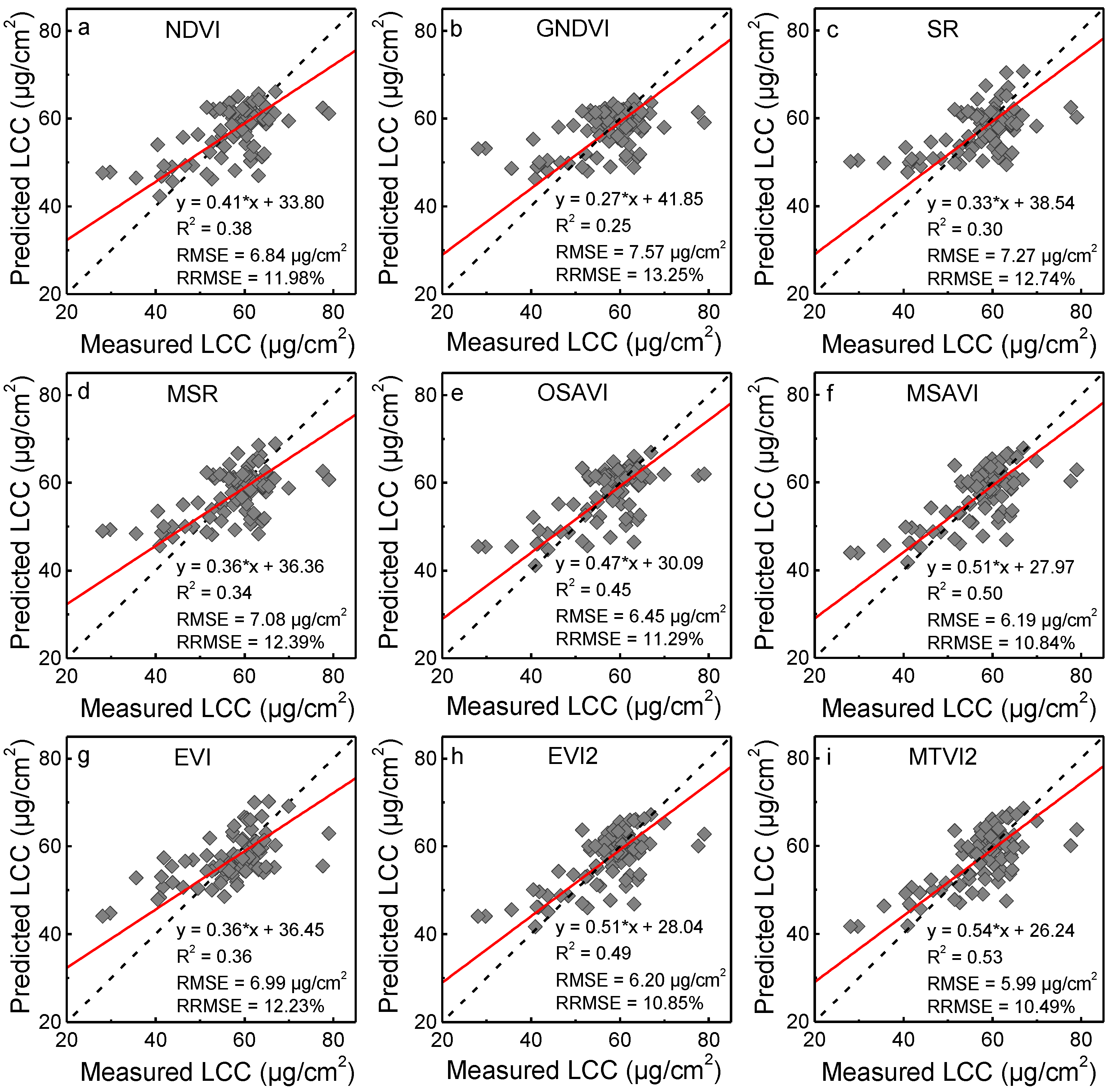
For LCC assessment, VIs that consisted of blue, green, red, and NIR bands were considered on account of the band settings of the Landsat-8 OLI sensor. Even though some VIs, for instance, MTVI2, MSAVI, and EVI2, were not intended for chlorophyll retrieval, they still exhibited good accuracy among all the VIs for LCC estimation. MTVI2 was constructed for increasing the sensitivity to the leaf area index while minimizing chlorophyll influence [38]. MSAVI aims to increase the dynamic range of vegetation signals and minimize soil background influences [37]. EVI2 was put forward to increase the sensitivity of vegetation features to high biomass regions while decoupling background signals and reducing atmosphere influences [35]. Compared with the performance of NDVI, these three indices showed much better results for LCC estimation, suggesting that the modifications of these three indices improved LCC estimation accuracies, particularly for MSAVI and EVI2 since they are composed of red and NIR bands, which is the same as NDVI. The center of the OLI red band is close to the absorption peaks of chlorophyll a and b at 662 nm and 644 nm [2], which could partly explain the good performance of these VIs. Furthermore, the LCC values used in this study were converted from SPAD readings, while SPAD readings were calculated from the transmission features of red (650 nm) and infrared (940 nm) light [49]. This could also account for the good performance of MTVI2, MSAVI and EVI2 in LCC estimation despite that their original purposes were not for LCC assessment. It is worth noting that combination of red and NIR bands showed better results than that of the combination of green and NIR bands since NDVI exhibited more accurate results than GNDVI. Overall, all these VI results suggest that red and NIR bands are critical for LCC assessment with Landsat-8 OLI data.

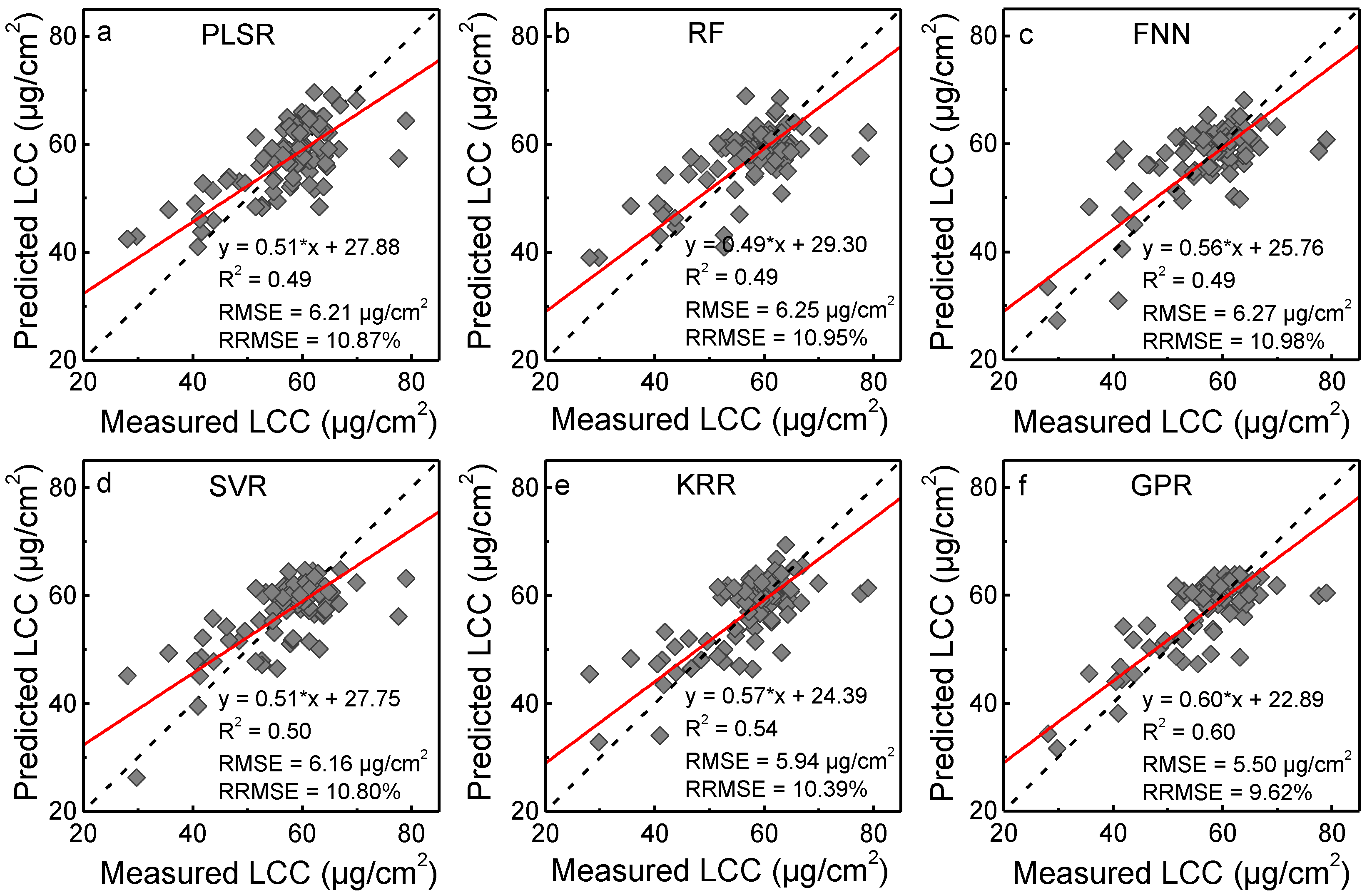
Compared with VI methods, MLRAs generally had slightly better results, since they utilized all band information and nonlinear transforms. NN gained attention for agronomic parameter modelling and operational products in previous studies [29,50,51]. Here, FNN did not outperform other MLRAs and showed a rather similar estimation to that of PLSR, RF, and SVR, suggesting that it might not be the most adequate algorithm. The methodologies of PLSR, RF, and SVR are different from each other, and they exhibited different performances for varied agronomy parameter retrieval in previous studies using hyperspectral data [4,52,53]. Here, they exhibited very similar estimation results. This might be attributed to the confined broadbands (i.e., 6 bands) used in these models. In comparison, KRR and GPR showed even better estimation results. These accurate results accord with their performance in previous research [54,55]. Among all MLRAs, GPR is the most capable for not only maintaining very good numerical performance and stability but also for largely overcoming the blackbox issue, by providing ranking features (bands) that are used in the model [14]. According to GPR sigma band analysis, we found that the red band and NIR band are the top two bands frequently used in GPR models, which indicates that these two bands are critical for GPR modeling. This could also support the phenomenon that VIs composed of red and NIR bands showed good results for LCC estimation.

In terms of LUT-based inversion methods, ten CFs with different multiple best solution regularization strategies showed varied behaviors for LCC retrieval. The results suggest that the “root mean square error” CF, which was extensively-used in some previous studies [56,57], might not be the optimal CF for LCC inversion with Landsat-8 OLI data since it exhibited rather poor estimation. In comparison, CFs such as “Pearson chi-square”, “Geman and McClure”, and “K(x) = −log (x) + x” that belong to three different families, had much better estimates. Among them, “K(x) = −log (x) + x” showed the best inversion accuracy. These results accord with the works of Rivera et al. [17] and Verrelst et al. [58]. The use of multiple solution regularization strategies did improve the inversion accuracy of different CFs as compared with the cases without using them. However, it seems that high values of multiple solutions were more effective than low values in regulating LUT-based inversion since most CFs achieved good estimations when high values of multiple solutions (i.e., 30%) were used. For noise regularization, a Gaussian noise model was used, and the same noise criterion (details in Section 2.4) was adopted for both LUT-based inversion methods and hybrid regression approaches, in order to make a comparison between them. Generally, LUT-based inversion methods were more effective than hybrid regression approaches in LCC retrieval with Landsat-8 OLI data, since LUT-based inversion methods with most CFs exhibited better LCC estimation. Reasons for this might be largely connected with the data sizes that were different in using these two methods: LUT-based inversion used all the simulated data (n = 121,500) for modelling, whilst partial simulation (n = 2500) was used for establishing hybrid regression models. Compared with the results from the full training data set with GPR, the use of AL methods with GPR led to superior retrieval accuracies, and all AL techniques actually exhibited similar estimation results for ground validation. AL methods from the diversity family showed consistent results for cross-validation and ground-validation processes, whereas the uncertainty AL exhibited quite a difference between the two processes, especially for the results of EQB with GPR, suggesting that it might be unstable though it achieved the best accuracy for ground-validation. Even though diversities existed between different ALs for training GPR models, we can conclude that AL approaches were fairly effective and accurate for LCC retrieval with hybrid regression methods.

5. Conclusions

In this study, the potential and capability of Landsat-8 OLI multispectral data for LCC assessment in winter wheat were comprehensively investigated and evaluated, using different retrieval methods including broadband VIs, MLRAs, LUT-based inversion, and hybrid regression approaches. Overall, the LCC estimation results exhibited good accuracies except variations existed between different retrieval methods. Among the selected VIs, MTVI2 showed the best estimation accuracy with an RMSE of 5.99 μg/cm² and an RRMSE of 10.49%. VIs (i.e., MSAVI, EVI2, OSAVI) established from red and NIR bands also exhibited good accuracy for LCC estimation. MLRAs generally had slightly better results compared to those of VIs. GPR best captured the variations in LCC with the highest accuracy for LCC retrieval (RMSE = 5.50 μg/cm², RRMSE = 9.62%). Furthermore, the red band and NIR bands outweighed other bands in GPR modelling, suggesting these two bands are of great importance for LCC retrieval. LUT-based inversion methods with different CFs exhibited varied results. “K(x) = −log (x) + x” CF that belongs to the “minimum contrast estimates” family had the best accuracy (RMSE = 8.08 μg/cm², RRMSE = 14.14%), followed by the “Pearson chi-square” and “Geman and McClure” CFs from “information measures” and “M-estimates” families, respectively. Moreover, the addition of multiple solution regularization strategies improved the inversion accuracy compared with the cases without using them. Owing to the computational cost and limited simulated data for modelling, hybrid regression methods with GPR exhibited inferior estimation compared to the results of LUT-based inversion. Nevertheless, the use of AL techniques together with GPR for LCC modelling significantly increased the estimation accuracy compared with the results from the full training data set with GPR, and the combination of EQB and GPR had the best accuracy for ground validation (RMSE = 12.43 μg/cm², RRMSE = 21.77%). On the basis of all tests carried out in this work with different retrieval methods, it can be concluded that Landsat-8 OLI multispectral data can be accurately used for crop LCC retrieval.

References

1. Project, G.C. International Geosphere-Biosphere Programme; IGBP: Stockholm, Sweden, 2010; Volume 21, p. 36. [Google Scholar]
2. Nobel, P.S. Physicochemical and Environmental Plant Physiology, 4th ed.; Elsevier Academic Press: Amsterdam, The Netherlands, 2009. [Google Scholar]
3. Haboudane, D.; Miller, J.R.; Tremblay, N.; Zarco-Tejada, P.J.; Dextraze, L. Integrated narrow-band vegetation indices for prediction of crop chlorophyll content for application to precision agriculture. Remote Sens. Environ. 2002, 81, 416–426. [Google Scholar] [CrossRef]
4. Yu, K.; Lenz-Wiedemann, V.; Chen, X.; Bareth, G. Estimating leaf chlorophyll of barley at different growth stages using spectral indices to reduce soil background and canopy structure effects. ISPRS J. Photogramm. Remote Sens. 2014, 97, 58–77. [Google Scholar] [CrossRef]
5. Gitelson, A.A.; Vina, A.; Ciganda, V.; Rundquist, D.C. Remote estimation of canopy chlorophyll content in crops. Geophys. Res. Lett. 2005, 32. [Google Scholar] [CrossRef] [Green Version]
6. Zhao, K.; Valle, D.; Popescu, S.; Zhang, X.; Malick, B. Hyperspectral remote sensing of plant biochemistry using Bayesian model averaging with variable and band selection. Remote Sens. Environ. 2013, 132, 102–119. [Google Scholar] [CrossRef]
7. Verrelst, J.; Munoz, J.; Alonso, L.; Delegido, J.; Pablo Rivera, J.; Camps-Valls, G.; Moreno, J. Machine learning regression algorithms for biophysical parameter retrieval: Opportunities for Sentinel-2 and -3. Remote Sens. Environ. 2012, 118, 127–139. [Google Scholar] [CrossRef]
8. Malenovsky, Z.; Homolova, L.; Zurita-Milla, R.; Lukes, P.; Kaplan, V.; Hanus, J.; Gastellu-Etchegorry, J.P.; Schaepman, M.E. Retrieval of spruce leaf chlorophyll content from airborne image data using continuum removal and radiative transfer. Remote Sens. Environ. 2013, 131, 85–102. [Google Scholar] [CrossRef] [Green Version]
9. Verrelst, J.; Pablo Rivera, J.; Veroustraete, F.; Munoz-Mari, J.; Clevers, J.G.P.W.; Camps-Valls, G.; Moreno, J. Experimental Sentinel-2 LAI estimation using parametric, non-parametric and physical retrieval methods—A comparison. ISPRS J. Photogramm. Remote Sens. 2015, 108, 260–272. [Google Scholar] [CrossRef]
10. Pu, R.; Gong, P. Hyperspectral Remote Sensing and Its Applications; Higher Education Press: Beijing, China, 2000. [Google Scholar]
11. Dash, J.; Curran, P.J. The MERIS terrestrial chlorophyll index. Int. J. Remote Sens. 2004, 25, 5403–5413. [Google Scholar] [CrossRef]
12. Verrelst, J.; Malenovsky, Z.; Van Der Tol, C.; Camps-Valls, G.; Gastellu Etchegorry, J.-P.; Lewis, P.; North, P.; Moreno, J. Quantifying Vegetation Biophysical Variables from Imaging Spectroscopy Data: A Review on Retrieval Methods. Surv. Geophys. 2019, 40, 589–629. [Google Scholar] [CrossRef] [Green Version]
13. Tang, X.G.; Song, K.S.; Liu, D.W.; Wang, Z.M.; Wang, Y.D. Comparison of Methods for Estimating Soybean Chlorophyll Content Based on Visual/Near Infrared Reflection Spectra. Spectrosc. Spectr. Anal. 2011, 31, 371–374. [Google Scholar]
14. Verrelst, J.; Alonso, L.; Rivera Caicedo, J.P.; Moreno, J.; Camps-Valls, G. Gaussian Process Retrieval of Chlorophyll Content From Imaging Spectroscopy Data. IEEE J. Sel. Top. Appl. Earth Obs. Remote Sens. 2013, 6, 867–874. [Google Scholar] [CrossRef]
15. Feret, J.B.; Francis, C.; Asner, G.P.; Gitelson, A.A.; Martin, R.E.; Bidel, L.P.R.; Ustin, S.L.; Le Maire, G.; Jacquemoud, S. PROSPECT-4 and 5: Advances in the leaf optical properties model separating photosynthetic pigments. Remote Sens. Environ. 2008, 112, 3030–3043. [Google Scholar] [CrossRef]
16. Darvishzadeh, R.; Matkan, A.A.; Ahangar, A.D. Inversion of a Radiative Transfer Model for Estimation of Rice Canopy Chlorophyll Content Using a Lookup-Table Approach. IEEE J. Sel. Top. Appl. Earth Obs. Remote Sens. 2012, 5, 1222–1230. [Google Scholar] [CrossRef] [Green Version]
17. Rivera, J.P.; Verrelst, J.; Leonenko, G.; Moreno, J. Multiple Cost Functions and Regularization Options for Improved Retrieval of Leaf Chlorophyll Content and LAI through Inversion of the PROSAIL Model. Remote Sens. 2013, 5, 3280–3304. [Google Scholar] [CrossRef] [Green Version]
18. Zhang, S.; Wang, Q. Inverse Retrieval of Chlorophyll from Reflected Spectra for Assimilating Branches of Drought-Tolerant Tamarix ramosissima. IEEE J. Sel. Top. Appl. Earth Obs. Remote Sens. 2015, 8, 1498–1505. [Google Scholar] [CrossRef]
19. Croft, H.; Arabian, J.; Chen, J.; Shang, J.; Liu, J. Mapping within-field leaf chlorophyll content in agricultural crops for nitrogen management using Landsat-8 imagery. Precis. Agric. 2019, 21, 1–25. [Google Scholar] [CrossRef] [Green Version]
20. Verrelst, J.; Dethier, S.; Rivera, J.P.; Munoz-Mari, J.; Camps-Valls, G.; Moreno, J. Active Learning Methods for Efficient Hybrid Biophysical Variable Retrieval. IEEE Geosci. Remote Sens. Lett. 2016, 13, 1012–1016. [Google Scholar] [CrossRef]
21. Upreti, D.; Huang, W.; Kong, W.; Pascucci, S.; Pignatti, S.; Zhou, X.; Ye, H.; Casa, R. A Comparison of Hybrid Machine Learning Algorithms for the Retrieval of Wheat Biophysical Variables from Sentinel-2. Remote Sens. 2019, 11, 481. [Google Scholar] [CrossRef] [Green Version]
22. Dorigo, W.A. Improving the Robustness of Cotton Status Characterisation by Radiative Transfer Model Inversion of Multi-Angular CHRIS/PROBA Data. IEEE J. Sel. Top. Appl. Earth Obs. Remote Sens. 2012, 5, 18–29. [Google Scholar] [CrossRef]
23. Roy, D.P.; Wulder, M.A.; Loveland, T.R.; Woodcock, C.E.; Zhu, Z. Landsat-8: Science and Product Vision for Terrestrial Global Change Research. Remote Sens. Environ. 2014, 145, 154–172. [Google Scholar] [CrossRef] [Green Version]
24. Houborg, R.; Mccabe, M.; Cescatti, A.; Gao, F.; Schull, M.; Gitelson, A. Joint leaf chlorophyll content and leaf area index retrieval from Landsat data using a regularized model inversion system (REGFLEC). Remote Sens. Environ. 2015, 159, 203–221. [Google Scholar] [CrossRef] [Green Version]
25. Croft, H.; Chen, J.M.; Zhang, Y.; Simic, A.; Noland, T.L.; Nesbitt, N.; Arabian, J. Evaluating leaf chlorophyll content prediction from multispectral remote sensing data within a physically-based modelling framework. ISPRS J. Photogramm. Remote Sens. 2015, 102, 85–95. [Google Scholar] [CrossRef]
26. Cerovic, Z.G.; Masdoumier, G.; Ghozlen, N.M.B.; Latouche, G. A new optical leaf-clip meter for simultaneous non-destructive assessment of leaf chlorophyll and epidermal flavonoids. Physiol. Plant. 2012, 146, 251–260. [Google Scholar] [CrossRef] [PubMed]
27. Verhoef, W.; Jia, L.; Xiao, Q.; Su, Z. Unified Optical-Thermal Four-Stream Radiative Transfer Theory for Homogeneous Vegetation Canopies. IEEE Trans. Geosci. Remote Sens. 2007, 45, 1808–1822. [Google Scholar] [CrossRef]
28. Campbell, G.S. Derivation of an angle density function for canopies with ellipsoidal leaf angle distributions. Agric. For. Meteorol. 1990, 49, 173–176. [Google Scholar] [CrossRef]
29. Weiss, M.; Baret, F. S2ToolBox Level 2 Products: LAI, FAPAR, FCOVER. 2016. Available online: https://step.esa.int/docs/extra/ATBD_S2ToolBox_L2B_V1.1.pdf (accessed on 24 June 2020).
30. Rouse, J.W.; Haas, R.H., Jr.; Schell, J.A.; Deering, D.W. Monitoring vegetation systems in the Great Plains with ERTS. In Third ERTS-1 Symposium; NASA: Washington, DC, USA, 1974; pp. 309–317. [Google Scholar]
31. Gitelson, A.A.; Kaufman, Y.J.; Merzlyak, M.N. Use of a green channel in remote sensing of global vegetation from EOS-MODIS. Remote Sens. Environ. 1996, 58, 289–298. [Google Scholar] [CrossRef]
32. Jordan, C.F. Derivation of Leaf-Area Index from Quality of Light on the Forest Floor. Ecology 1969, 50, 663–666. [Google Scholar] [CrossRef]
33. Chen, J.M. Evaluation of Vegetation Indices and a Modified Simple Ratio for Boreal Applications. Can. J. Remote Sens. 1996, 22, 229–242. [Google Scholar] [CrossRef]
34. Liu, H.Q.; Huete, A.R. A feedback based modification of the NDVI to minimize canopy background and atmospheric noise. IEEE Trans. Geosci. Remote Sens. 1995, 33, 457–465. [Google Scholar] [CrossRef]
35. Jiang, Z.; Huete, A.R.; Didan, K.; Miura, T. Development of a two-band enhanced vegetation index without a blue band. Remote Sens. Environ. 2008, 112, 3833–3845. [Google Scholar] [CrossRef]
36. Rondeaux, G.; Steven, M.; Baret, F. Optimization of soil-adjusted vegetation indices. Remote Sens. Environ. 1996, 55, 95–107. [Google Scholar] [CrossRef]
37. Qi, J.; Chehbouni, A.; Huete, A.R.; Kerr, Y.H.; Sorooshian, S. A modified soil adjusted vegetation index. Remote Sens. Environ. 1994, 48, 119–126. [Google Scholar] [CrossRef]
38. Haboudane, D.; Miller, J.R.; Pattey, E.; Zarco-Tejada, P.J.; Strachan, I.B. Hyperspectral vegetation indices and novel algorithms for predicting green LAI of crop canopies: Modeling and validation in the context of precision agriculture. Remote Sens. Environ. 2004, 90, 337–352. [Google Scholar] [CrossRef]
39. Geladi, P.; Kowalski, B.R. Partial Least-Squares Regression: A Tutorial. Anal. Chim. Acta 1986, 185, 1–17. [Google Scholar] [CrossRef]
40. Breiman, L. Random Forests. Mach. Learn. 2001, 45, 5–32. [Google Scholar] [CrossRef] [Green Version]
41. Hagan, M.T.; Menhaj, M.B. Training feedforward networks with the Marquardt algorithm. IEEE Trans. Neural Netw. 1994, 5, 989–993. [Google Scholar] [CrossRef]
42. Vapnik, V.; Golowich, S.; Smola, A. Support Vector Method for Function Approximation, Regression Estimation, and Signal Processing. Adv. Neural Inf. Process. Syst. 1997, 9, 281–287. [Google Scholar]
43. Suykens, J.A.K.; Vandewalle, J. Least Squares Support Vector Machine Classifiers. Neural Process. Lett. 1999, 9, 293–300. [Google Scholar] [CrossRef]
44. Rasmussen, C.E.; Williams, C.K.I. Gaussian Processes for Machine Learning; The MIT Press: New York, NY, USA, 2006. [Google Scholar]
45. Li, H.; Chen, Z.X.; Jiang, Z.W.; Wen-Bin, W.U.; Ren, J.Q.; Liu, B.; Hasi, T. Comparative analysis of GF-1, HJ-1, and Landsat-8 data for estimating the leaf area index of winter wheat. J. Integr. Agric. 2017, 16, 266–285. [Google Scholar] [CrossRef]
46. Lessio, A.; Fissore, V.; Borgognomondino, E. Preliminary Tests and Results Concerning Integration of Sentinel-2 and Landsat-8 OLI for Crop Monitoring. J. Imaging 2017, 3, 49. [Google Scholar] [CrossRef] [Green Version]
47. Meng, Q.; Zhang, L.; Xie, Q.; Yao, S.; Chen, X.; Zhang, Y. Combined Use of GF-3 and Landsat-8 Satellite Data for Soil Moisture Retrieval over Agricultural Areas Using Artificial Neural Network. Adv. Meteorol. 2018, 2018, 1–11. [Google Scholar] [CrossRef]
48. Yin, C.; He, B.; Quan, X.; Liao, Z. Chlorophyll content estimation in arid grasslands from Landsat-8 OLI data. Int. J. Remote Sens. 2016, 37, 615–632. [Google Scholar] [CrossRef]
49. Markwell, J.; Osterman, J.C.; Mitchell, J.L. Calibration of the Minolta SPAD-502 leaf chlorophyll meter. Photosynth. Res. 1995, 46, 467–472. [Google Scholar] [CrossRef] [PubMed]
50. Verger, A.; Baret, F.; Weiss, M. Performances of neural networks for deriving LAI estimates from existing CYCLOPES and MODIS products. Remote Sens. Environ. 2008, 112, 2789–2803. [Google Scholar] [CrossRef]
51. Verger, A.; Baret, F.; Camacho, F. Optimal modalities for radiative transfer-neural network estimation of canopy biophysical characteristics: Evaluation over an agricultural area with CHRIS/PROBA observations. Remote Sens. Environ. 2011, 115, 415–426. [Google Scholar] [CrossRef]
52. Pullanagari, R.R.; Kereszturi, G.; Yule, I.J. Mapping of macro and micro nutrients of mixed pastures using airborne AisaFENIX hyperspectral imagery. ISPRS J. Photogramm. Remote Sens. 2016, 117, 1–10. [Google Scholar] [CrossRef]
53. Han, Z.; Zhu, X.; Fang, X.; Wang, Z.; Wang, L.; Zhao, G. Hyperspectral estimation of apple tree canopy LAI based on SVM and RF regression. Spectrosc. Spectr. Anal. 2016, 3, 800–805. [Google Scholar]
54. Rivera, J.; Verrelst, J.; Delegido, J.; Moreno, J. On the Semi-Automatic Retrieval of Biophysical Parameters Based on Spectral Index Optimization. Remote Sens. 2014, 6, 4927–4951. [Google Scholar] [CrossRef] [Green Version]
55. Campos-Taberne, M.; Garcia-Haro, F.; Camps-Valls, G.; Grau-Muedra, G.; Nutini, F.; Crema, A.; Boschetti, M. Multitemporal and multiresolution leaf area index retrieval for operational local rice crop monitoring. Remote Sens. Environ. 2016, 187, 102–118. [Google Scholar] [CrossRef]
56. Kempeneers, P.; Zarco-tejada, P.J.; North, P.R.; Backer, S.D.; Delalieux, S.; Sepulcre-Canto, G.; Morales, F.; Aardt, J.A.N.V.; Sagardoy, R.; Coppin, P.; et al. Model inversion for chlorophyll estimation in open canopies from hyperspectral imagery. Int. J. Remote Sens. 2008, 29, 5093–5111. [Google Scholar] [CrossRef]
57. Zhang, Y.; Chen, J.M.; Miller, J.R.; Norland, T.L. Leaf chlorophyll content retrieval from airborne hyperspectral remote sensing imagery. Remote Sens. Environ. 2008, 112, 3234–3247. [Google Scholar] [CrossRef]
58. Verrelst, J.; Rivera, J.P.; Leonenko, G.; Alonso, L. Optimizing LUT-Based RTM Inversion for Semiautomatic Mapping of Crop Biophysical Parameters from Sentinel-2 and -3 Data: Role of Cost Functions. IEEE Trans. Geosci. Remote Sens. 2014, 52, 257–269. [Google Scholar] [CrossRef]
Figure 1. Location of the study site (standard true-color composite of a Landsat-8 OLI image) and the distribution of elementary sampling units (ESUs).
Remotesensing 12 02574 g001
Figure 2. A schematic diagram of leaf chlorophyll content (LCC) retrieval methods adopted in the present study.
Remotesensing 12 02574 g002
Figure 3. Cross-validation results of different VIs for LCC assessment. (ai) are results for NDVI, GNDVI, SR, MSR, OSAVI, MSAVI, EVI, EVI2, and MTVI2, respectively.
Remotesensing 12 02574 g003
Figure 4. Cross-validation results of different MLRAs for LCC estimation. (af) are results for PLSR, RF, FNN, SVR, KRR, and GPR, respectively.
Remotesensing 12 02574 g004