A Method for the Estimation of Finely-Grained Temporal Spatial Human Population Density Distributions Based on Cell Phone Call Detail Records

Abstract

Estimating and mapping population distributions dynamically at a city-wide spatial scale, including those covering suburban areas, has profound, practical, applications such as urban and transportation planning, public safety warning, disaster impact assessment and epidemiological modelling, which benefits governments, merchants and citizens. More recently, call detail record (CDR) of mobile phone data has been used to estimate human population distributions. However, there is a key challenge that the accuracy of such a method is difficult to validate because there is no ground truth data for the dynamic population density distribution in time scales such as hourly. In this study, we present a simple and accurate method to generate more finely grained temporal-spatial population density distributions based upon CDR data. We designed an experiment to test our method based upon the use of a deep convolutional generative adversarial network (DCGAN). In this experiment, the highest spatial resolution of every grid cell is 125 $\times$ 125 square metre, while the temporal resolution can vary from minutes to hours with varying accuracy. To demonstrate our method, we present an application of how to map the estimated population density distribution dynamically for CDR big data from Beijing, choosing a half hour as the temporal resolution. Finally, in order to cross-check previous studies that claim the population distribution at nighttime (from 8 p.m. to 8 a.m. on the next day) mapped by Beijing census data are similar to the ground truth data, we estimated the baseline distribution, first, based upon records in CDRs. Second, we estimate a baseline distribution based upon Global Navigation Satellite System (GNSS) data. The results also show the Root Mean Square Error (RMSE) is about 5000 while the two baseline distributions mentioned above have an RMSE of over 13,500. Our estimation method provides a fast and simple process to map people’s actual density distributions at a more finely grained, i.e., hourly, temporal resolution.

1. Introduction

The dynamic nature of temporal and spatial population distributions has a profound impact on urban and transportation planning [1,2,3], safety for human crowds [4,5,6], disaster impact assessment [7,8,9], human activity-travel behaviour [10,11] and epidemiological modelling [12,13,14]. However, when studying human activity on a city-wide scale, estimating and mapping more detailed population distributions at higher than a 12h temporal resolution is still a challenge [15]. More detailed population distribution models with a higher spatial and temporal resolution have many applications. For example, prediction of the population distribution can provide local authorities with contextual data and suggestions to avoid or alleviate stampede events [6,16]. In metropolises, especially in Chinese cities, there are plenty of shared bicycles to serve citizens which can be improved by dynamically provisioning the resources according to people’s distributions [17]. Another case concerns take-away food outlets and markets, if these are aware of where and when the population is distributed at a higher or lower density, they can arrange for the goods and labour force resources to be distributed, dynamically and more effectively, to generate a higher profit [18].

The traditional way used by authorities to determine the population distribution is to take a population census. However, this is quite static and normally takes place only at relatively large time intervals such as decades [19]. Most recently, an increasing number of studies using mobile phone data have been undertaken by many academic researchers and companies to estimate and map the population distribution more dynamically. Such studies tend to use mobile phones, in part because of the 100% penetration rate of mobile phones in many global regions [20], and because they embed location-based sensors such as for a Global Navigation Satellite System (GNSS). However, it is hard to collect such GNSS data large scale such as for a nation. Further, such data may be privacy invasive even if anonymised as private information such as someone’s home location can be easily discerned. A less privacy invasive method is to analyse mobile phone access points or base-station call detail records (CDRs) [15,21,22,23]. A CDR includes the location information of the cell. However, the location accuracy is less privacy invasive as we can only detect if the phone is in range of a base station, typically of the order of 400-800 m in urban areas. To meet the requirements for population dynamic distribution at a higher temporal resolution, hourly or minutely, estimations based on CDR data can be made.

However, the analysis of CDR data faces several key challenges. The definition of night and day for people’s activity varies. For example, the traditional definition of night-time and daytime (night and day) is daytime is from sunrise to sunset, and night-time is from sunset to sunrise. However, in this study we focus on differences in people’s activities between night and day, which may have no obvious critical transition between these. Thus, Rein Ahas et al. redefined ‘midnight’, ’morning start’, ’midday’ and ’duration of day’ based on the mobile telephone usage of residents rather than solar or standard time, which is more useful to determine the distribution of temporal activities in cities and monitoring urban changes with georeferenced mobile phone data [24]. Mobile phone users’ distributions determined using CDRs may not equate well to the actual population at different times. For example, people always call more frequently during daytime than at night, so less records are generated and stored in the CDRs dataset at night. Therefore, if we only use the mobile phone users or the records number to present actual people, it would miss many people who do not use their phone at night and this can cause a large error in determining the actual population distribution. Thus, how to convert the mobile phone CDR data into actual population density distribution effectively, is challenging. In our study, we present a population distribution process where we generate an artificial population density distribution and process this to validate the estimated population distribution. Thus, the novel contributions of this paper are as follows.

(1)

We present a simple method to estimate dynamic, actual, people’s density distributions, effectively, based on CDR data.

(2)

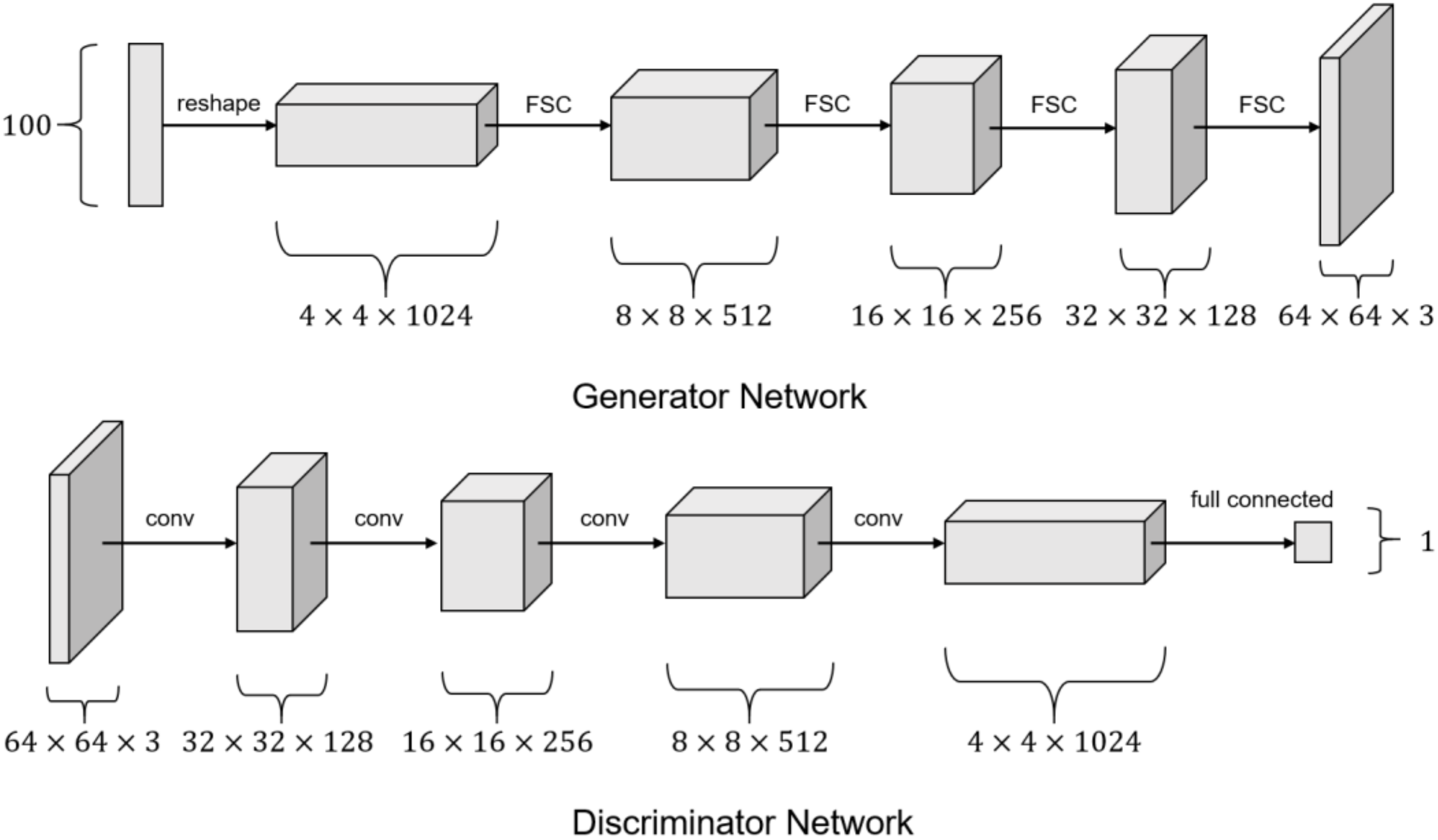
We specify an experimental framework to test the robustness and accuracy of our estimation method using artificial people’s density distributions generated by a deep learning method using a deep convolutional generative adversarial network (DCGAN).

(3)

Our estimation method can provide a faster, simpler process to estimate and map out actual people’s density distributions at an hourly temporal resolution, which can be used to understand people’s dynamic hot-spots or crowd distributions in large, city-wide, urban areas.

The remainder of this article is organized as follows: Section 2 reviews related work. Section 3 presents the mobile phone dataset and the main estimation method. Results and discussion are reported in Section 4. In Section 5, we present our conclusions and our thoughts for future research.

2. Related Work

The traditional method used by governments and authorities to obtain the population density in a large space is a census, which is accurate, but it only gives a static population distribution in every period cycle, typically every 10 years [19]. The spatial resolution of a census is coarse- to medium-grained and reflects areas at its best resolution such as towns with an area of about 15 km² (in the UK). Remote sensing has been actively explored as a means to study population distribution [25,26,27], however, using only remote sensing data has resulted in mapped population densities that are not dynamic because of the slow periodic pass-over and scanning rate of such satellites for the same area, which often limits the applicability of such data for use in fine-scale applications, e.g., territorial planning [27], which cannot do hourly population estimates in 400 by 400 m areas. Obtaining the population distribution at a smaller scale area can be estimated using video surveillance [28] or images [29], however, it is only suitable for a small space and is very challenging to scale up to a city-wide scale.

There are some studies to explore the relationship between mobile phone users and actual population and to (create a) map (of) the population distribution more dynamically. Deville et al. [21] found a special relationship between mobile phone call record density and actual population density from the census as follows:

$$\mathsf{\rho }=\mathsf{\alpha }{\sigma }^{\beta }$$

(1)

where $\mathsf{\rho }$ represents the census population density while $\sigma$ represents the mobile phone call record density, and $\mathsf{\alpha }$, $\mathsf{\beta }$ are the coefficient constants they estimated. However, this cannot be used to estimate and map directly actual populations because $\mathsf{\alpha }$ and $\beta$ vary in time and space but there is only one census population distribution taken in that time period. Zhang et al. [15] presented an estimation and mapping method using machine learning to predict mobile phone users’ locations and then converted and mapped population distributions based upon the above formula. However, the formula is not suitable for dynamic population distributions. Increasingly, as mobile phones get more powerful they can also support a Geographic Information System (GIS) [30] themselves, locally, by providing geographic information such as coordinate of mobile phone users based on Global Positioning System (GPS) sensors inside, via a communications network and the interaction with other mobile applications. Some studies [15,21], give very coarse-grained time population estimations such as separating each whole day into two parts, daytime from 7:00 a.m. to 8:00 p.m. and nighttime from 8:00 p.m. to next day 7:00 a.m. but the definition of what is day versus night can be quite variable. Ricciato et al. presented a methodology to enable the fusion of cell-level and area-level data from heterogeneous data sources and considered a novel tessellation scheme based on cell coverage maps, instead of cell tower locations [22]. However, their method works on simulations of population—there is no validation against actual population density estimations and mapping.

Fine grained population estimation has been a focus of several studies. Bakillah et al. presented an alternative approach for fine-resolution population mapping for building level areal interpolation based on volunteered geographic information (VGI) data [31]. They also use other datasets such as land use/land cover, and points of interest (POI) datasets to refine the population estimation at the building level. This study also presented a far-reaching case for population estimations, but the validation part is missed and the contributions are not devoted to dynamic estimation. Liu and Pollmann combined static census data and anonymised mobility data to estimate a dynamic population based upon a Bayesian model [32]. Their estimation results are at a spatial resolution of 1 km and a temporal resolution of 1 h. However, the temporal resolution in this study, fixed at 1 h, could be finer because the sampling time for mobile data could be as short as 1 s. Validation of the method is also an issue as there is no actual or similar dynamic ground truth data used in the study.

Multi-agent system (MAS), which is a computerized system, consists of multiple interacting intelligent agents to tackle problems that are difficult or impossible for an individual agent to solve, have also been used to model the dynamics of human distributions in cities. In a large spatial scale such as city, Itzhak [33] presented a multi-agent simulation model of the population dynamics in a city, which operated with a two-layer structure including city’s housing infrastructure and free agents to represent individual citizens. At a small scale, such as indoor rooms and social housing accommodation communities, agent-based modelling (ABM) appears to be applicable for the evacuation in crowd stampedes and flow management in traffic [34]. Another study conceptualizes and specifies a multi-agent system, called Land-Use Dynamics Simulator (LUDAS), representing the human–landscape use in rural forest margins. This is used to explore alternative scenarios to improve livelihoods and mitigate against the negative impact of land-use changes, thereby supporting the negotiation process amongst various stakeholders in land-use planning [35]. In addition to land-use, climate change is also regarded as a key impact factor that influences population flows, and the paper illustrates how agent-based models incorporating a Theory of Planned Behaviour, can be used to project evidence based future changes in migration, in response to future demographic, economic social and climate changes [36]. However, such MASs tend not to be validated against any ground truth data of the dynamic actual population distributions at large spatial scales and at a higher temporal resolution such as hours.

To summarise, a key challenge for researchers is first to access data at a city-wide scale at a fine spatial and temporal resolution that is not privacy invasive, e.g., CDR data sets from a phone operator. Second, such CDR data sets when they are shared, tend to not be for the current time period (i.e., they are several years old) which makes it difficult to cross-validate against other data sources that offer indirect evidence of current dynamic population distributions, e.g., social media data tend to be generally available only for the current time period. Hence, what is needed is some way to link different population distribution methods that may cover different time periods, i.e., what is needed is a population mapper or artificial population generator to help facilitate this. A promising technique to do this is to use a generative adversarial network (GAN) framework for estimating generative models via an adversarial process, in which two models: a generative model G that captures the data distribution, and a discriminative model D that estimates the probability that a sample comes from the training data rather than from G. This deep learning model could be used to train types of image, which can represent population distributions, and to generate artificial ones. Further, a class of convolutional neural networks (CNNs) called deep convolutional generative adversarial networks (DCGANs) that have certain architectural constraints, has been introduced to bridge the gap between the success of CNNs for supervised learning, and unsupervised learning based on GANs [37]. GAN and DCGAN have been tested to be effective in generating ’realistic’ artificial images, e.g., faces and even music [37]. Distribution maps can be represented as images to be used for training in DCGAN and to generate artificial population distributions.

3. Data and Method

In this section, we first present our methodology by giving an overview (Figure 1). The last part in this section introduce the datasets, and then following the overview, the method is described, part by part. In the next section, Section 4, results and discussion, we still follow the overview shown in this section, to illustrate the results step by step with a discussion.

There are two main parts to the study in this paper: the first main part involves a cross-check that CDR driven population distributions are valid and a second part is to demonstrate a general application of CDR-driven population models, e.g., for a city in China. There are a total 6 steps in the two parts (see Figure 1). In the first part, we have four steps. The first step is to use DCGAN to train and generate artificial population density distributions based on the ground truth distribution, which is defined as the distribution that is equal to or very close to the actual people population distribution, from the Tencent company (http://www.tencent.com/en-us/index.html) in China. This company released some datasets of key cities in China for academic and commercial purposes, which can provide GNSS-based positioning information in city scale of their users, who have agreed to share their location. Thus, we can use such a dataset to represent the ground truth population distributions. More information of the dataset is introduced in Section 3.1.1. In the second step, we randomly extract sample points to represent the CDRs. Then in step 3, our method is utilised to map out the estimated population density from the CDR and in the final step, 4, we use a cosine similarity method to validate that the two distributions (estimated CDR and Tencent generated one) are similar enough, and named this as comparison 1.

In the second part, we apply our estimation method to the actual CDRs of Beijing, China, to map and analyse the dynamic population distributions. Although, it could be argued just to use the Tencent data for population distribution analysis and not to bother using the CDR data, Web companies tend to be regional or to have coldspots where there is much less data, whereas CDR data is global, e.g., Tencent Web services currently only dominates in China where Google (https://about.google/) for example has far less users. Hence, our focus is on CDR-driven population distributions which have more global applicability. There are 2 steps in this part, step 5 estimates the population density distribution in Beijing, China, and then step 6 uses the census data as comparison 2 or as an additional cross-check of the results.

3.1. Data

3.1.1. Tencent Positioning Big Data

As a cross-check that the population distributions generated from one source, e.g., CDRs, are valid, we can compare these against the population distributions generated from other data sources such as from Web applications from Web companies, e.g., Tencent. WeChat from Tencent Company is currently the most popular social software in China, and according to the WeChat Annual Data Report 2018 (http://media.people.com.cn/n1/2019/0110/c40606-30513560.html), there has been more than 1.01 billion users who logon to WeChat every day. In larger cities in China such as Beijing, Shanghai and Guangzhou, the penetration rate of WeChat has reached at least 96% of citizens according to Kantar China Social Media Impact Report 2018 (https://cn-en.kantar.com/media/social/2018/kantar-china-social-media-impact-report-2018/). In addition to WeChat software, there are several other mobile applications produced by Tencent Company such as social application QQ, Tencent Video and QQ Browser which are also popular with high penetration rates. All these applications need their users to turn on positioning permissions so that Tencent Company can get the location of users using their smart phone GNSS once one of them is installed. Based upon the data of users’ location, Tencent presents a real-time platform to show the heat map of their users (https://heat.qq.com/index.php) and the density distributions can be easily mapped by GIS software such as ArcGIS (https://www.esri.com/en-us/arcgis/about-arcgis/overview). Based on the penetration rates and the user number of Tencent applications, the Tencent positioning big data represents a ground truth data of the actual people population density distribution in China, especially in larger cities.

The spatial structure of the Tencent positioning data consists of evenly distributed vector points that are stored as a SHP format file (https://desktop.arcgis.com/en/arcmap/10.3/manage-data/shapefiles/what-is-a-shapefile.htm). Under the projected coordinate system of WGS 1984 World Mercator (https://desktop.arcgis.com/en/arcmap/latest/map/projections/mercator.htm), they are arranged evenly as shown in Figure 2, each point is 5566 metres away from an adjacent point in the east or west direction (Figure 2, W-E Line), while 7235 metres away from a point in the north or south direction (Figure 2, N-S Line). For each SHP file, there are millions of points that cover the whole of China at a specific time, for example, 6:00 A.M, 01 September 2019. For each point, there is a feature called Recorded Number of People (RNP) that represents the recorded number of people, at this point, at this time. In order to convert the points to a people density distribution, we use a kernel density estimation (KDE) method [38] that can be processed in ArcGIS to estimate the hourly density distribution covering the whole of China. The spatial resolution of the output maps is set as 100 metres. Then the hourly Tencent people density distribution raster maps of China can be generated.

Although Tencent positioning big data are closer to the ground truth for the population distribution, we could not use the historical data that covers the same period of CDR data of Beijing in 2015 for this Tencent platform as this just provides current not historical data views. It is difficult to compare GNSS data with CDR data because the CDR data we use, is a historical dataset. This is because CDR providers do not generally provide the latest data to 3rd parties only samples of historical data. In contrast, the GNSS dataset provider, an instant message network and web service provider, does not provide historical data only the current data, and even they only provide limited demo historical data for academic and commercial purposes. Thus, the two historical datasets of CDR and Tencent ones are hard to overlap in both time and space. Hence, GNSS and CDR data are not available for the same period. However, the DCGAN method can solve the problem, because when we train the GNSS data, we do not need to consider time (see Section 3.2.1). Further, we think this is also an important strength of our approach, which presents a promising method to solve a data fusion problem when different datasets are obtained at different times.

Note also the analysis of Web service, e.g., Tencent data, exhibits the same temporal coldspots as CDR records where people may sleep at night and not use their communication devices to access the Web. We get the distributions of hourly Tencent people density from 20:00 April 29 to 15:00 April 30 (20 h) per city (Beijing, Nanjing and Shanghai), which are a total 60 distributions. For each distribution, we use a 20 km $\times$ 20 km frame (window) that is randomly moved in the distribution for 100 times, and then extract 100 sub-distributions to get a total 6000 sub-distributions ($100\times 60=6000$). In the last part of the paper, we just call the 6000 sub-distributions as 6000 distributions. Here we show the distributions, rendered as 15 level greyscale images with an equal density value (samples are shown as Figure 3). The datasets are used to train the model and then generate artificial people density distribution by DCGAN and then to take the Population Distribution Process part aa shown in Figure 1.

3.1.2. Call Detail Records Data from Beijing, China

We used anonymised, individual, actual, call detail records (CDR) from the China Mobile operator company (Beijing) (https://www.bloomberg.com/profile/company/JLCBHZ:CH) to generate population distributions for analysis after having cross-checked them against a population distribution generated from another source, e.g., Tencent data. A CDR contains information (shown in

Table 1. CDR structure.

ID	Name	Description
1	Timestamp	Interactive time of users and base station
2	CI	Corresponding base station’s id
3	IMSI	Encrypted ID of users

): for the International Mobile Subscriber Identification Number (IMSI), that is an international unique code for every SIM card or Home Location Register (HLR) or Visitor Location Register (VLR) to recognize users on the network; timestamp records when the interactive events happen; Cell Identity (CI) corresponding to the base-station location when recording. The dataset that was collected is anonymised for use in scientific research whenever an otherwise identifiable user calls or sends a text message provided by his or her Chinese mobile phone operator, recording a new data record. The dataset for this study includes over 4.8 billion records of more than 300 million users on 1 sample day, e.g., Thursday 17 February, 2015 in Beijing, China.

We used the locations of all the 51,216 mobile base stations shown in Global System for Mobile Communication (GSM) engineering parameters inner structure (

Table 2. The inner structure of Global System for Mobile Communication (GSM) engineering parameters.

ID	Name	Description
1	CI	Unique ID of base station
2	Lat, Lon	Latitude and longitude of base-station location

). However, there are plenty of base stations that are so close to each other such that their identified latitude and longitude are the same, hence, we combined such similar location base stations to be the same, thus reducing the base-station number to about a third of the original, from 51,216 to 17,445. The coverage area of each mobile base station can be approximated as a Voronoi polygon that is built around it. When a phone is used to make a call or send a text message, its location is found via being in range of the specific mobile base station to which the phone is connected.

The CI, IMSI and the Timestamp for users in every record that is identified by an IMSI also identifies the corresponding base-station location, taken as the location of the user. The accuracy of the Timestamp in CDRs is the temporal resolution of recording and is within 1 s. The CDRs are stored in one Comma-Separated Values (CSV) file every 1 h (3600 s). In space, the density of the base station covers a circle area with a radius of 100-500m. While in suburban areas, where this is impacted by the requirements and terrain to support sufficient subscribers, a single station covers a bigger circle area with a radius of about 500m to 1000m. In the next section, we will introduce the process that supports the four steps of the CDR driven population distribution estimation shown in Figure 1.

3.1.3. Census Data of Beijing, China

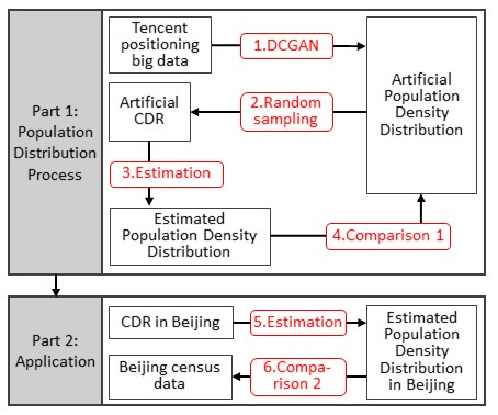
In this study, we use the Beijing census data in 2010 (Available from http://www.bjstats.gov.cn/; retrieved 01/05/2019) to compare the distribution from CDRs. Figure 4 shows the Beijing population density distribution for its 322 administrative units in 2010.

3.2. Method

3.2.1. Part 1, Step 1: Building Artificial Distributions Based on a DCGAN

To test our estimation method, we need some ground truth data to compare our estimation with. However, because there is no real ground truth available to match the date of our CDR data, we devised a process whereby an artificial people’s distribution is generated, and then use our estimation method to map the distribution from the artificial CDR that is sampled from artificial people points. In this study, we use Tencent positioning dataset to provide the ground truth data of people’s distribution for the training data, then build a DCGAN to generate an artificial distribution in the next step of the process. As a result that our method does not consider the impact of different times to estimate population distribution, dynamic migration flow and pattern changes with respect to time are not needed in the comparison process. Thus, a static distribution with the characteristics of population distribution pattern is what we aim for in this step.

A DCGAN model includes two parts, a generator and a discriminator. The architecture of the generator and the discriminator in a DCGAN model is shown in Figure 5, where in the generator network, a 100-dimensional uniform distribution is projected to a small spatial extent convolutional representation and a series of four fractionally-strided convolutions that can reconstruct the image’s spatial resolution and then performs the convolution, to convert this high level representation into a 64 × 64 pixel image, while the discriminator network does the opposite.

Moreover, the generator network takes random noise as input, then runs the noise through the differentiable function (neural network) to transform the noise and reshape it to have a recognizable structure similar to the images in the training dataset. The output of the generator is determined by the choice of the input random noise. Running the generator network over several different random input noises results in different realistic output images. The end goal of the generator is to learn a distribution similar to the distribution of the training dataset output realistic images. To be able to do so, the generator network needs to be trained.

A discriminator network is a basic classifier network that outputs the probability of an image to be real. Therefore, during the training process, the discriminator network is shown real images from the training set half the time and fake images from the generator for another half of the time. The discriminator target is to assign a probability near 1, for real images and probability near 0, for fake images. On the other hand, generator tries the opposite, its target is to generate fake images, for which the discriminator would result in a probability close to 1 (considering them to be real images from the training set). As training goes on, the discriminator will become better at classifying real and fake images. Therefore, to fool the discriminator, the generator will be forced to improve to produce more realistic samples.

The training distribution images are from Beijing, Nanjing and Shanghai cities as shown in Figure 3, based on the corresponding Tencent positioning data. As a result that people’s distributions have similar fractal characteristics in space [39], which means population have quite distinct fractal structure in that its distributions are self-similar across many orders or scales, we mix these three typical cities in China to train to generate a universal distribution for this process. Then, we follow the original set of the DCGAN from [37] with a learning rate of 0.0002, batch size 64 $\times$ 64, the training dataset is the extracted 6000 maps for an input image size set to 108 $\times$ 108 pixels in greyscale. We train the sampled maps with 1000 epochs, and finally generated 64 artificial population distributions as images.

In the next step, we selected 10 from of these 64 results for the next step in the process for cross-checking. For each selected artificial distribution, a random point is generated according to the greyscale colours on the image, representing the density of the population density, for example, if we define that there are 500,000 people in this area, the same number of points is put on the map according to the value of each pixel of an image. For the final generated artificial distribution, we designate these as the baseline Artificial Population Density Distributions.

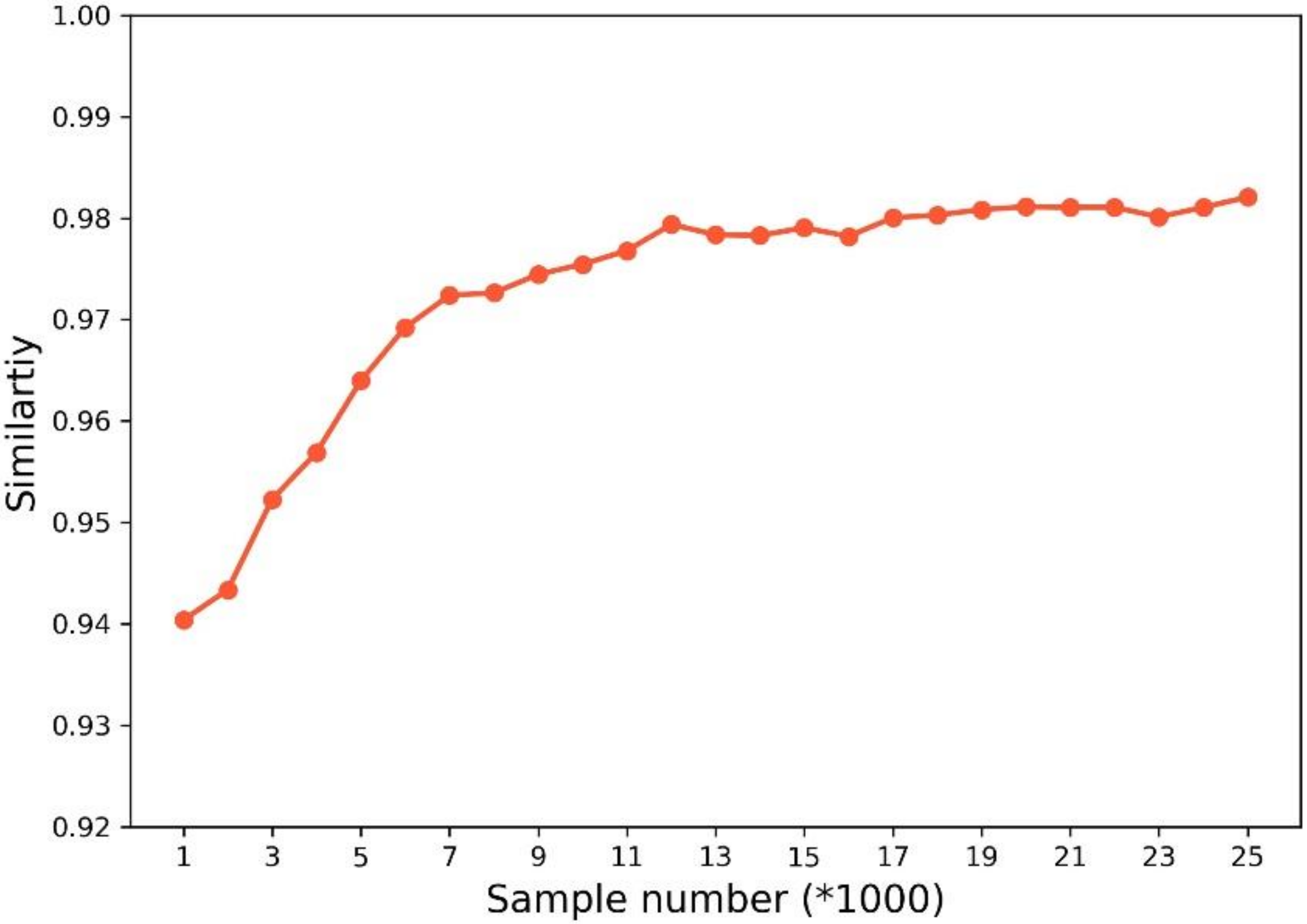
3.2.2. Part 1, Step 2: Random Sampling of CDR

We regard mobile phone users who have been recorded in CDR as the random sample for actual people in this study, thus, specific numbers of people act as points in the baseline distribution, defined as a ground truth distribution used for comparison, in this step.

We randomly sample the artificial distributions to generate artificial CDRs. The temporal and spatial extent of our distributions are configurable. It is in part 2, when we apply the method to a specific space and time that we can for example configure the time resolution to be 2 min (at the start of every two hours) as an example. We take a sub-sample of the 2 h data as this is a representative sample of it and allows us to reduce the computation cost, which is a key characteristic of our method.

We also need to build an artificial base-station distribution, which means the base stations in our artificial environment are distributed similarly to the actual ones. In order to make the population distribution process closer to the real situation, the actual region extracted from Beijing with the base-station distribution, is selected to be the test area. In addition, the proportion of the population number in the process and actual population number (we set to be ${\mathrm{P}}_{process}$) should be equal to the proportion of a test region with respect to the whole area of Beijing. The ratio of the selected base-station number and the number of base stations in the whole of Beijing also needs to be approximately equal to this proportion.

In our study, the area of a region is a square with a side length of 20 km, where the number of inside base stations is about 425 (425/17445 is equal to 400/14.41 thousand km², the 14.41 thousand is the area of whole Beijing). The process of choosing a region has 2 steps: first, we set a big square that can surround the whole Beijing with the smallest area; second, we set the smaller square with a side length of 20 km and let it move from the left top to right top step by step and every step is 1 km, then move down one step from left to right, and then move down one step again, until the small square has moved to the right bottom of the big square. At the same time, we count the base-station number for every step, and finally, the most suitable one that has the closest number to 425 base stations has been found. Finally, the most suitable area has been determined which is shown in Figure 6, and we define this area as the study sample region. The structure of the area distribution for all Voronoi polygons is shown in Figure 7, which can illustrate the similarity of the two regions to make the experiment equate closer to the actual situation. Hence, now, the baseline Artificial Population Density Distribution and base-station distribution are built completely.

3.2.3. Part 1, Step 3: Population Distribution Estimation Method

This gives the details of our estimation method in our experiment. Before introducing this, we present the conditions and assumptions that our estimation method is based upon. As a result that the population number in some cites is growing or decreasing slowly over years, the population distribution changes over one or several years can be ignored. In big cities, especially those that attract many tourists, the population changes over days are relatively stable and related to the number of permanent residents. For example, according to the comprehensive statistics of the immigration and border inspections conducted by the China National Immigration Bureau in the first quarter of 2015, from January 1, 2015 to March 31, 2015, the number of people going out from Beijing was 62,321,614, while going in to Beijing was 62,447,662 (Available from http://www.mps.gov.cn/n2254996/n2255000/n2255031/c4904063/content.html, retrieved 01/03/2019). The two numbers are really close and based on the results released by the Beijing Statistical Bureau, the permanent population of Beijing in 2015 was 21.705 million (Available from http://www.bjstats.gov.cn/tjsj/cysj/201511/t20151109_311727.html, retrieved 01/03/2019), the average rate of change in the total daily population of Beijing is only 0.5%. Thus, the population can be regarded as a bounded dataset, i.e., for an enclosed area, when only the population number, and not individual information such as the age and gender, are considered. In this situation, although people move from one place to another place all the time, this happens within an enclosed area.

Based upon the presupposition of population stability at a city scale as described above, we start to introduce the details of this estimation method. First, based on the precondition that the study area is an enclosed region with a fixed people number $N_a$, we extract an equal number $N_s$ of mobile users randomly according to IMSI code from CDRs over each time point covering the time duration we study. Second, we count the total number of mobile phone users in each base-station polygon (as shown in Figure 1). Third, we use the total number of people $N_a$ in this area to divide by $N_s$ to get a constant $M$, and then normalise every mobile phone users’ dataset extracted from CDRs, by $M$. Hence, $M$ points are randomly put on the map within each base-station region. Finally, a KDE method is utilised to output the estimated population density distribution. More details concerning this are given as follows.

In our study, we regard the base-station location that records the calling or texting events as the location for mobile phone users. A Thiessen polygon algorithm [40] was utilised to create a Voronoi polygon for each mobile phone base station in order to define the location of phone users within a district (Figure 1). According to the previous analysis, based on the presupposition of a stable population density at a city scale, we regard that mobile phone users’ interactions with base stations as random events, which means that mobile phone users are randomly sampled people who are just recorded by base stations. Thus, we could use the sampled people to estimate the whole people population. In terms of the time scales selected, if we want to obtain the estimated population distribution in a certain time, we can extract the mobile phone users by the identified features (CI) defined in Table 2 during this period to represent a sample of actual people.

$$M=\frac{N_a}{N_s}$$

(2)

After setting up the mobile phone user number, which is also regarded as the sampling number, the proportion of the sampling people and the whole of people is calculated. As shown in Equation (2), $M$ is the multiple of $N_a$ the actual population number is divided by $N_s$,where $N_s$ is the sampling people number, which also is the number of mobile phone users. Then we get the location of the sampled people and the summation $N_i$ within each Voronoi polygon, and $\mathrm{i}$ represents the ID for each polygon. The same number of $N_i$ after being multiplied by $M$ is input as the random points which are to be generated within responding Voronoi polygon. The total number of points equals the actual total population number as taken from the census data and used as the ground truth data, as shown as Equation (3). Finally, we use a KDE method to create a map of the spatial density of the estimated people distribution.

$$N_a=M{\displaystyle \sum }_{i=1}^n{N}_i$$

(3)

To process a KDE, an appropriate search radius is calculated using Geographic Information System (GIS) software, e.g., ArcGIS (Available from https://www.arcgis.com/index.html, retrieved 01/03/2019) to produce an estimation of the density at different spatial resolutions and produce a raster grid consisting of 100m by 100m square cells. Although we can model changes in population density cells in time as people move (flow) between adjacent cells. As 1 cell has 8 neighbouring cells, it is not so clearly identifiable in this step, between which adjacent cells the flow actually occurs for the case when several changes in population density in adjacent cells occur at the same time.

The GIS-based KDE estimation method uses a moving window to calculate and output a point or line density of each grid cell. Given that the sample $\left(x_1,x_2,\dots ,x_n\right)$, is an independent identically distributed sample extracted from the population with a distribution density function $f$, at a point $x$, $f\left(x\right)$, calculated using a Rosenblatt–Parzen kernel [41,42] estimate:

$$f_n\left(x\right)=\frac{1}{nh}{{\displaystyle \sum }}_{i=1}^{n}k\left(\frac{x-x_i}{h}\right)$$

(4)

where $k()$ is the kernel function; h > 0 is a smoothing parameter for the kernel called the bandwidth; $\left(x-x_i\right)$ is the distance from the estimated point x to a sample point $x_i$.

When KDE is processed, the determination or selection of the bandwidth h has a great influence on the calculation result. As h increases, the change of the point density in the space is smoother but the density structure is masked. When h is reduced, the estimated dot density change can start to change abruptly between adjacent Voronoi polygons.

The specific steps for KDE estimation are: (1) define a search radius to count the number of events; (2) determine the output raster size based upon the density accuracy requirements; (3) calculate the density contribution of each event to each grid in the circular domain by the kernel function; (4) assign the density value of each raster to the value of the density contribution of each event in the raster search radius; (5) output the density values for each raster grid.

In this study we determine the characteristics of the population density distribution for the Beijing city area within 800m as the default radius, the spatial resolution is 100 metres per cell when using the ArcGIS10.5 kernel density analysis tool (Available from http://desktop.arcgis.com/en/arcmap/10.5/tools/spatial-analyst-toolbox/how-kernel-density-works.htm, retrieved 01/03/2019). Furthermore, in this process when we use this tool, the “in_features” parameter means the input features (point or line) used to calculate the density, is set as the people point SHP file (Available from https://desktop.arcgis.com/en/arcmap/10.3/manage-data/shapefiles/what-is-a-shapefile.htm, retrieved 02/02/2020). The “method” parameter determines whether or not to use a shortest path on a spheroid (geodesic) or a flat earth (planar) view is set as planar because all of our operated map features are under a projected coordinate system. Finally, the “population_field” which denotes the population values for each feature is set as none because every point represents one person without any other features.

3.2.4. Part 1, Step 4: Comparison 1 of Artificial Actual and Estimated Population Distributions

A raster grid is output after using KDE with the density value in each cell. After the process described above, the estimated people’s density distributions are generated in a raster grid format. As a result that the baseline distribution is generated from the images that are predicted by DCGAN, to compare the baseline distribution with the estimated distribution, the raster grids need to be converted to images, which means the colour or greyscale assignment system of the renderer in the symbology process, is realised using ArcGIS (Available from https://pro.arcgis.com/en/pro-app/help/mapping/layer-properties/symbolize-feature-layers.htm, retrieved 01/03/2019). The generated baseline images are output with a 108 $\times$ 108 pixels resolution in a greyscale. To make a cell in the image represent a geographic unit more easily, according to the First Law of Geography [43], "everything is related to everything else, but near things are more related than distant things", we resize generated images in a 200 $\times$ 200 resolution greyscale by the nearest-neighbour interpolation method. The equation of the method is given below:

$$pixe\_B\left(X,Y\right)=pixe\_A\left(X\times \left(m/M\right),Y\times \left(n/N\right)\right)$$

(5)

where the size of the source image A is $m\times n$, and the size of the scaled image B is $M\times N$, the pixel value at the (X, Y) position of the scaled image B is the pixel value at $\left(X\times \left(\frac{m}{M}\right),Y\times \left(\frac{n}{N}\right)\right)$, of the source image A. It is worth mentioning that although the images have been scaled, the population density distribution estimation would hardly have been influenced because the resizing process just impacts the quality of the artificial maps, while all the next steps are based on them, compared with these maps directly, so the resizing of artificial maps has little effect on the estimated results.

We also converted the grids of estimated distribution into the same size, where every pixel represents a square area with a 100 m side length; the degree of the greyscale means the density of people per square kilometre.

Then we use a standard cosine similarity method to measure the similarity value for the two images, using the following standard equation:

$$\mathrm{S}=\cos \left(\mathsf{\theta }\right)=\frac{A·B}{\parallel A\parallel \parallel B\parallel }=\frac{{{\displaystyle \sum }}_i^n{A}_i\times B_i}{\sqrt{{{\displaystyle \sum }}_i^n{\left(A_i\right)}^2}\times \sqrt{{{\displaystyle \sum }}_i^n{\left(B_i\right)}^2}}$$

(6)

where $\mathrm{S}$ is the similarity of the two images $A$ and $B$; $A_i$ represents the value of i-th value of image $A$, while $B_i$ represents the value of i-th value of image $B$, which are the density values in this study. After converting the pixel values in images A and B into vectors, the final cosine similarity results are obtained by calculating the ratios of the cumulative point products of those ${\ell }_2$ norms. The maximum value of $\mathrm{S}$ is 1. In this normalised range of 0–1, the smaller the value is, the greater the image difference is.

The artificial distributions are generated by DCGAN and are regarded as the ground truth; while the estimated distributions are the results that are computed by our method. The artificial distribution region and the estimated distribution region are the same.

3.2.5. Part 2, Steps 5 and 6: Application in Beijing

In this part we apply our estimation method on an actual CDR dataset of Beijing, China. There are two steps in this part: step 5 uses our estimation method to apply on the actual CDRs in Beijing; then in step 6 we validate the estimation results.

One of the most difficult things in the estimation of population density distribution is that the accuracy of such a method is difficult to validate because there are no ground truth data for the dynamic population density distribution in time scales such as hourly. This is also the reason why we present an application of a deep learning method to create an artificial population density distribution, which is a novelty of our paper. Thus, in the application part of this paper, we just use the real CDR data to apply our method on a real case. Thus, we deploy another method as cross-check 2, (step 6 of part 2) called comparison 2, to compare the CDR distributions against the static census population distributions at nighttime (00:00 to 8:00 a.m. and 22:00 to 12:00 p.m.) because the people distribution in this period is relatively static, which has been used in papers [15,21]. The results of using this part are reported in Section 4.2.

4. Results and Discussion

In this part we present and discuss the results with respect to the overview of Figure 1, step by step. It is worth mentioning first off that from the 64 results (as shown in Figure 9) generated by DCGAN, we randomly selected 10 of them to take the distribution process to test the robustness of our method. After assessing the results and discussion, we applied the method to the whole area of Beijing, and mapped the half hourly dynamic estimated population density distributions over a day.

4.1. Part1: Results of the Process

4.1.1. Step 1: Generated Images and Baseline Distribution

In the DCGAN process, the discriminator loss quantifies how well the discriminator is able to distinguish real images from fake ones. The loss in this section uses the mean squared error loss function in the Tensorflow framework (Available from https://www.tensorflow.org/tutorials/generative/dcgan, retrieved 01/05/2020). It compares a discriminator’s predictions on real images to an array of 1s, and the discriminator’s predictions on fake (generated) images to an array of 0 s. The generator’s loss quantifies how well it was able to trick the discriminator.

Intuitively, if the generator is performing well, the discriminator will classify the fake images as real (or 1). Figure 8 shows the details of the discriminator loss and generator loss, against epochs, increasing when we used DCGAN to train and generate the artificial population distributions. The generator loss (g_loss) fluctuates strongly at the start during the epochs increasing from 1 to 50. At the same time, the discriminator loss (d_loss) fluctuates with a high frequency. Then after 50 epochs, though there are still medium fluctuations happening in both networks, they reach a stable point of about 0.3 for the g_loss when the epoch reaches about 200, which implies that the discriminator then tends to detect fake images as real. The discriminator loss decreases at the start and keeps stable at about 4 when the epoch reaches to 200. This loss convergence would normally signify that the model reaches an optimum, where it has improved such that it has learnt well enough, resulting in a reliable artificial distribution to test our estimation method.

The artificial distributions are shown in Figure 9. The 6000 maps are the training data to input into the DCGAN, and then DCGAN generates 64 new artificial maps. The output number of the artificial map number is a parameter of DCGAN, we set the model to generate 64 ones. In these 64 results of the artificial distribution, there are several maps that appear non-sensical, for example, too much of a white area over dense people distribution and too much of a black area the over sparse people distribution. These are unrealistic according to our experience. Excluding these non-sensical distributions, others meet the conditions of the population distribution in China, where the spatial distribution of the population has the characteristics of a "ring" and "radial" and these overlap (mixed "ring" and "radial") [44]. Thus, after excluding some of the non-sensical cases, we select 10 of remaining distributions randomly to process in the next steps (step 2 to step 4).

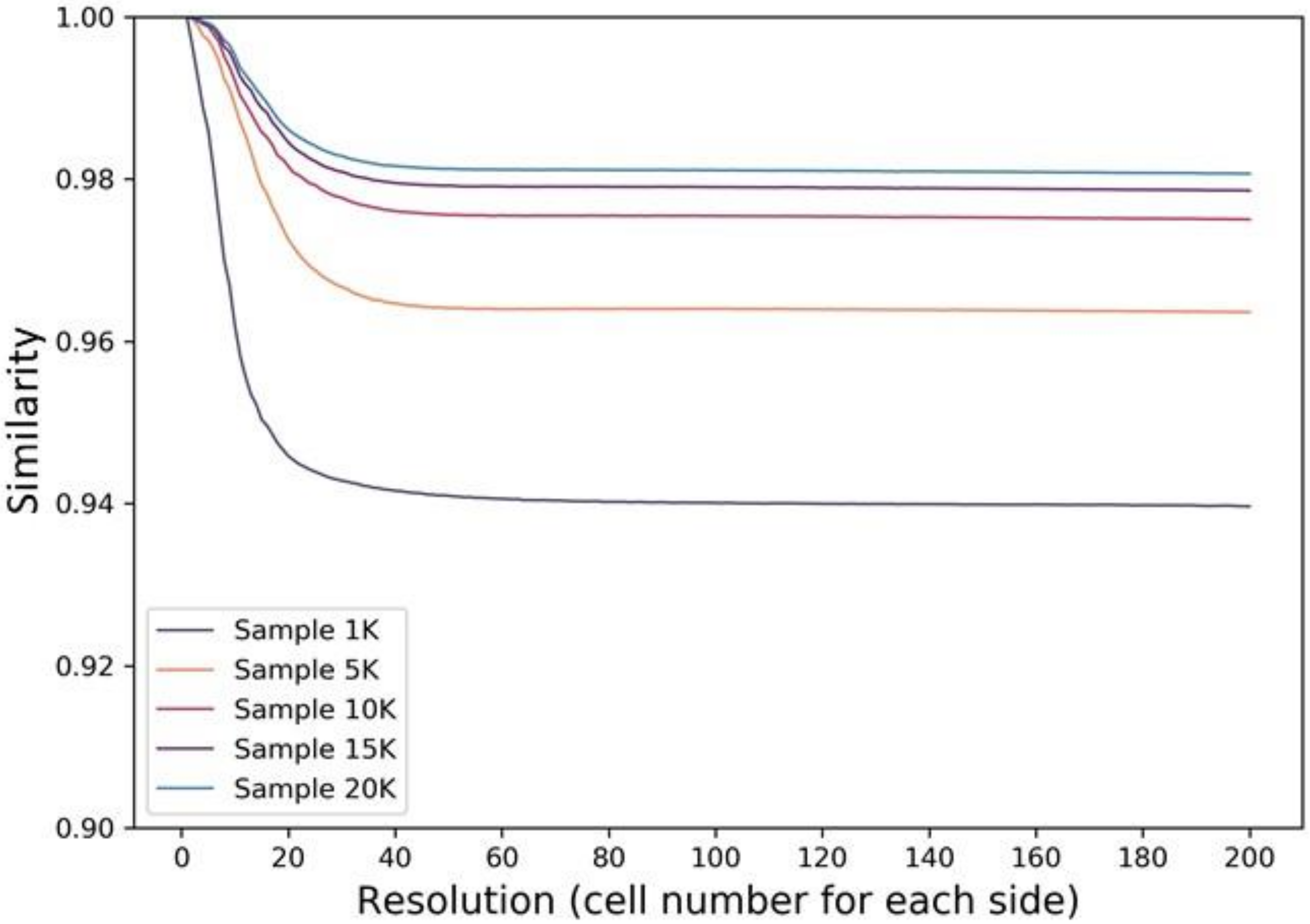
4.1.2. Step 2-3: Estimation Process

In order to facilitate the uniform processing of the image data, we render all images into a greyscale, where the white areas mean a higher value and the black ones mean a lower value. After that we get 10 baseline people density distributions. The next step is to put random points into the map according to the density distribution. As discussed previously, we put 500,000 points into the corresponding map where one point represents one real person. We extract the sample points randomly as the mobile phone users who have interacted with base stations and who are recorded in the artificial CDRs.

In order to detect the relationship between the sampling number and estimated results, we set a different sampling number from 1000 to 25,000, and create maps of the raster density images. Then following the process that has been described in Section 3.2.3., for each sampling points group, first, we count the total number of artificial mobile phone users (extracted from the artificial CDRs) in each base-station polygon (as shown in Figure 6). Second, we use the total number of people $N_a$ in this area, divided by $N_s$ to get a constant $M$. Then, we normalise every artificial mobile phone users’ dataset extracted from artificial CDRs by dividing by $M$. Hence, $M$ points are randomly put on the map within each base-station region. Finally, the KDE method is utilised to output the estimated population density distribution.

This process has been repeated 10 times to get 10 different results. Figure 10 shows an example of the baseline distribution and the corresponding estimation results using different sample numbers from 1000 to 10,000 points. Finally, we compare each image with the baseline greyscale maps.

4.1.3. Step 4: Comparison 1

Figure 11 shows the results of average similarity for 10 artificial images with an increasing sample number. As the input images increase with a sampling number from 1000 to 12,000, the average similarity index grows dramatically, while after 12,000, the values are stable at about 0.982. We also calculated the similarity index when the sampling number is 500,000 that is equal to the artificial generated number of people, which means all generated data were used in our method. The average comparison result for 10 groups is 98.5% based upon a cosine similarity test. However, in a real situation, it is impossible to get a 100% similarity agreement because of the reasons that have been explained previously, for example, not all mobile phone users interact with the base station within a specific period.

When calculating the similarity index using a cosine similarity method, the resolution of an input image can be changed. The maximum input image resolution is 200 $\times$ 200 in the initial image, while the minimum input image resolution is 1 $\times$ 1, which means when the input image is put into the model and the resolution is set as 1 $\times$ 1, the image would has only 1 value that is the average value of the 200$\times$ 200 cells. If we set the resolution as another value, for example, 2 $\times$ 2, the input image would consist of 4 square cells and everyone has the value of the average of 100 $\times$ 100 cells. This is applied to both the original artificial distributions and estimated distributions. The process is illustrated in Figure 12.

Through changing the input resolution from 1 $\times$ 1 to 200 $\times$ 200, which is the cell number along one square image side, the similarity index was calculated at the same time.

Figure 13 illustrates the average relationship between similarity and input resolution for different sample numbers: 1000, 5000, 10,000, 15,000 and 20,000. As the input resolution increases, the similarity decreases gradually from approximately 1 to a stable value that depends on the sample size, which is represented by the same average grey level of all pixels of the two (artificial and estimated real) distributions. When the resolution increases to 50 $\times$ 50 cells, the similarity index reaches the lowest point, which is decided by the sample number. Note for all the different samples, all lines keep a stable similarity index from 50 $\times$ 50 until a resolution of 200 $\times$ 200. As a result that we set each pixel to represent 100 metres (20,000 km/200=100 km) when using KDE, according to Figure 13, the spatial resolution of our estimation method can be as high as 125 metres (20,000 km/160=125 km). When the geographic length of each side cell is less than 125 metres, the similarity index is stable. This means that when outputting the final density map using KDE, the cell size is set as 125 metres as it is a needless waste of computer memory and CPU to make a raster side length shorter than 125 metres. We do not need to let the resolution be equal to the GNSS resolution because the relation is limited by the coarser resolution of the base-stations’ location estimations.

If more accurate results are required, more points could be sampled. The estimation results with a different sample number illustrates the different levels capability that estimate the density distribution of the method. In the next section, we will use our method with a specific sample number and KDE output geographic cell size for Beijing to map half hourly population density distributions over one specific (test) day using the mobile phone CDR data.

4.2. Part2: An Application in Beijing

Here we represent a case study of Beijing, China, based on the actual CDR data in 2015 to show an application of our method. In Section 4.2.1, we analyse the actual CDRs of Beijing, then in Section 4.2.2, we use our estimation method to estimate the actual population density. In Section 4.2.3, we use the comparison 2 strategy to show the estimation capability of our method.

4.2.1. The Extraction and Analysis of Mobile Phone Users in CDRs

The CDR dataset of Beijing on Thursday February 17, 2015 is used as an application of our method. According to the analysis in Section 1, we know that in the first quarter of 2015, from January 1, 2015 to March 31, 2015, the number of people going out from Beijing was 62,321,614, while going into Beijing was 62,447,662. The two numbers are close and based on the results released by Beijing Statistical Bureau, the permanent population of Beijing in 2015 was 21.705 million, the average rate of change in the total daily population of Beijing is only 0.5%. Thus, we regard Beijing as an enclosed city whose population number is stable over a day without needing to consider the mobility of each individual.

When using our method, the sample population should first be extracted from CDRs. However, the average frequency of mobile phone users using their phone throughout a whole day varies, i.e., less people use their phone at nighttime such as at 2:00 a.m., while more people use their phone at daytime such as at 10 a.m. Every time, people use their phone to call or text, the device interacts with the base station that records this event, called an event station–user interaction event. Then, the mobile phone users in the first 30s per 1 h on February 17th in CDRs is counted and then we calculate the event frequency using the equation:

$$\mathrm{f}=\frac{\mathrm{N}}{\mathrm{t}}$$

(7)

where N is the number of mobile phone unique users, and t is 30 s. The relationship between base-station–user interactive frequency and time over a day is shown as Figure 14. It is clear that from the start of the day, less people tend to call or text until 7:00 a.m., while it increases dramatically between 7:00 a.m. and 10:00 a.m. There is a little fluctuation during the next 8 h and the call frequency falls down rapidly from 18:00 pm until the end of the day.

The bar chart (Figure 14) shows how accuracy is affected by the sampling duration. For example, consider a sampling duration of one second every hour at the start of the hour, at 2:00 a.m., only 70,000 people were recorded in CDRs in the first second of 2:00 a.m., which means that if we want to estimate the actual population density distribution in this second, the $M$ in Equation (2) is 310 (total population number of Beijing 21,700,000 divided by 70,000). The recorded number of users account for 0.3% of total number, which corresponds to the sample number 1.5 $\times$ 1000 in Figure 11; the corresponding similarity is relative lower. However, if we extract the number of unique mobile phone users in an hour from 2:00 a.m. to 3:00 a.m., the total number of mobile phone users is about 1000,000 (it is much less than 3600 times 70,000, which equals 252,000, because there is large number of repeat users between each couple of continuous seconds), which corresponds to sample 24,000 in Figure 13, the accuracy of the population density estimation by our method is much higher. In contrast, at 10:00 a.m. for the sample day, 240,000 people were recorded in CDRs on the first second at 10:00a.m., the $M$ in Equation (2) is 90 (total population number of Beijing 21,700,000 divided by 240,000). The number of the recorded users accounts for 1.1% of the Beijing population, which corresponds to the sampling number 5.5 $\times$ 1000 in Figure 11 and the corresponding similarity is relatively lower. Meanwhile, if we extract the number of unique mobile phone users in an hour from 10:00 a.m. to 11:00 a.m., the total number of mobile phone user is much more than the number in one second, resulting in a much higher accuracy of the estimation. Thus, in order to reach a higher accuracy with a higher sample number of mobile phone users, the sampling duration at the start of 2:00 a.m. should be longer than the one starting from 10:00 a.m. In other words, if we extract the same sampling duration such as 1 min, the estimation accuracy of the duration starting from 2:00 a.m. would be lower than that from 10:00 a.m. From above, a different sampling time duration means a different accuracy in the estimation method, hence, we also define that temporal resolution in our method.

In our study, the number of mobile phone users in the sample is fixed at 100,000 over a whole day, which means that the sample ratio of mobile phone users to the whole population in Beijing is 0.4%, corresponding to the 2000 sampling number with a 0.94 similarity in Figure 13. Based on the sampling rate, the lowest sampling resolution could be 2 min at 2:00 a.m. and 30 s at 10:00 a.m. In order to map a dynamic estimation of the population density distribution with a regular time interval, mobile phone users in every first 2 min per half hour are extracted to be mapped. Although we could have mapped those using a more finely grained temporal resolution such as 2 min over a whole day, or mapped those by sampling more mobile phones users with a higher estimated accuracy. In this section we just show our quick estimation process as an example by mapping the dynamic population density distribution changing over a day in a spatial scale. Two minutes seems to be a good choice that balances the accuracy of a low sampled time with a reduction in the computing time.

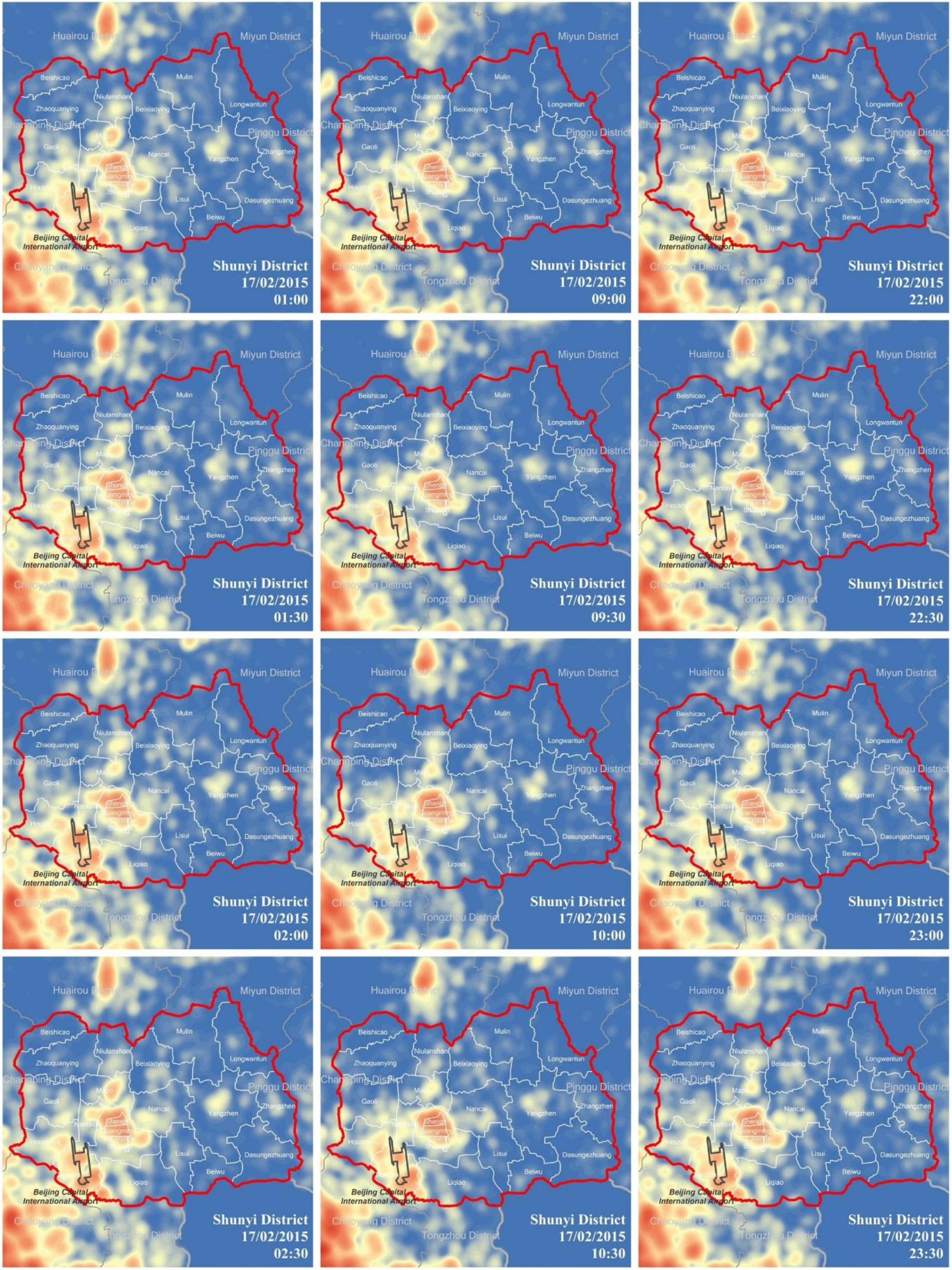
4.2.2. Dynamic Estimation of Half Hourly Temporal Population Density Distribution

After extracting mobile phone users as sampled people in Beijing on 17th February, 2015, the corresponding CI was used to identify the location of users for 48 times every half hour in the day. As per the process in Section 3.2, the sample number in this part is 100,000 while the population number in the whole of Beijing is 21,700,000, which is 217 times the number of points. In each Voronoi polygon, the same number of points was generated randomly within the associated polygon to represent people. Then a KDE method was used on the points distribution for 48 times to map the density distribution raster grids with a cell size of 125 $\times$ 125 square metres. Finally, according to the first grid at 00:00 a.m. on 17/02/2015, the maximum and minimum density values were separated into 32 classes (32 is the maximum number of classifications for raster grid using the symbology system in ArcGIS 10.5) by a geometric interval method (Available from https://pro.arcgis.com/en/pro-app/help/mapping/layer-properties/data-classification-methods.htm, retrieved 01/03/2019) and rendered using colour, where red means the higher density and where blue means a lower density. This was done for each of the grids.

Figure 15 shows the estimated population density distribution in Beijing on 17/2/2015 at a higher spatial resolution of every 2 h for the whole day. It can be seen that over the 24 h of the day, the density distribution changes dynamically in different areas. For example, in central Beijing such as in the Dongcheng District and Xicheng District, the people density is much higher than in suburban areas such as Miyun District and Huairou District during a day. In each administration district, the people density distribution is much higher in the centre town of the district than in its other arears. For example, in Huairou town, the centre of Huairou District in the north of Beijing, the people density is much higher there while the density is much lower in most surrounding towns such as Yanqi town that lies to the north of Huairou town, because there are large mountain areas in this town where less people live. People are more scattered at nighttime such as 2:00 a.m., while they cluster more tightly at daytime such as 11:00 a.m. This is because most of the workplaces are in central Beijing, however, here, there is less affordable residential land so that many people have to buy their apartments in suburban areas that have lower house prices. Thus, in suburban areas, there is a higher density of people at nighttime but a lower density at daytime, as people tend to spend more time at home when they away from work. In contrast, a lower people density at nighttime but a higher density during daytime is characteristic in urban areas that are the main workplaces during work time, on weekdays.

A similar distribution pattern occurs in each independent administration district. For example, as an urban–rural integration area, the Shunyi District is located in east Beijing. This contains the busiest airport in Asia in terms of passenger traffic and total traffic movements, Beijing Capital International Airport is located at the southwest of the Shunyi District and is close to the Chaoyang District (Figure 16). Figure 17 illustrates the changes of estimated population density distribution over several hours of the day. Comparing 3 images at each row (we grouped those into 4 rows and each one has 3 images on a sequential chronological order from left to right), it is clear that at night time such as from 1:00 to 2:00 a.m., more yellow patterns that represent a middle level population density are scattered in a larger spatial region while many of those are replaced by blue patterns that represent a lower population density at 9:00 to 10:00 A.M, such as in Beixiaoying town in the north of Shunyi District and Liqiao town in the south of the district. While at the centre of the district including Shengli street, Guangming street and Renhe street (the administration street has the same level as a town in this district), the red patterns means that a high population density grows deeper between 2:00 a.m. to 10:00 a.m., while it lessens slightly at the end of the day. This means in the daytime especially during work hours, people are very concentrated in the centre area of the district but when away from work or at nighttime, citizens tend to go back home and this results in a more scattered distribution pattern during this period. However, when we examine the Beijing Capital International Airport area (including the inner region of the airport and surround regions around the airport), the patterns of density distribution change less over the day, and the average density within this area over time sequence is more stable. This is because as the world’s second busiest airport in terms of passenger traffic since 2010 (Available from https://aci.aero/news/2019/03/13/preliminary-world-airport-traffic-rankings-released/, retrieved 01/03/2019), the uninterrupted flow of people who booked flights lead to the population density in this area changes less, keeping it stable at a relatively high level, including the people who work at the terminals and others who stay at hotels surrounding the airport.

4.2.3. Comparison 2: Results Are Compared with the Single Users/Records Number in CDRs

We extracted 2 min of CDRs starting from each 2 h on 17 February, 2015 during 00:00 and 8:00, and at 22:00, which forms 6 datasets. For each dataset, we create three maps of distributions. We regard every single record as one person to map to the first distribution (D1). We extract all mobile phone users recorded on CDRs to map the second distribution (D2), and finally we use our method to estimate and map the third distribution (D3).

Then, in terms of the administrative units of Beijing, we calculate the mean density from the three distribution maps within each unit. There are 2 steps in this process. First, we intersect the grid with all units. Every unit would consist one or more shards of cell, which means several neighbour cells would be divided by the 4 sides of a square unit to compose another shape of the unit, the cell or cells may be an integral square or irregular polygon, we record the number of the shards as $n$; second, for every unit we accumulate the density of each shard, using the equation below:

$$De{n}_{admin}={\displaystyle \sum }_{i=1}^{n}De{n}_i\times A_i/A_{admin}$$

(8)

where $De{n}_{admin}$ is the population density of every administrative unit, $i$ is the index n shards, $De{n}_i$ is the estimated density value of shard $i$, $A_i$ is the area of shard $i$ and $A_{admin}$ is the area of this administrative unit. Finally, we obtain the estimated population density for every administrative unit.

Comparing the three distributions with the census distribution respectively is the final step. The left part of the ’violin shaped’ plot shown in Figure 18b illustrates the mean density values of the estimation result for 322 administrative units, while the red part is the census data. Comparing these two parts of the density values, it is clear that they are very similar and that the estimated distribution is relatively stable over the 6 time frames, which agrees with the census data. The average population density in the 322 units from the census data is 8402.954 people per square kilometre, while the estimation ones are 7307.027, 6842.985, 6640.536, 7032.846, 7763.540 and 7368.336 on the times 00:00, 02:00, 04:00, 06:00, 08:00 and 22:00 February 17, 2015. However, the density mapped from single records number and users’ number with location features is much lower than the census because the CDRs we extracted are less. Although it shows that the number of CDRs extracted from a short time are not enough for these two traditional mapping methods, if the objective is to map population distribution in a short time with less computation time], our estimation method is effective to do this.

At the same time, Figure 18a illustrates the RMSE result for the three distribution results and census data over the 6 time ranges at nighttime, where the RMSE is about 5000 for the estimation method and is about 13,500 for the other two distributions. The big difference has 2 main causes, the first is the incomplete sampling in D1 and D2, because there is much less people who are using their phones at nighttime. The second concerns the 60% market share (Available from https://cn-en.kantar.com/media/mobile/2015/smartphone-penetration-rate-jumps/, retrieved 02/02/2020) of the China Mobile operator company from where we got our CDR dataset. However, in our method, we solve this issue by using the ratio of the number of sampled people to actual population number. Our method in this step shows two obvious advantages, first, it can eliminate the big difference between the gap mentioned above, second, by using our method we do not need to consider the influence of the Telecom company market share that provides the CDR data. The results of the comparison of RMSE demonstrate that simple mobile phone users and CDR number cannot represent the actual population.

In terms of comparison with the work of Deville et al. [21], we use CDRs to estimate the actual dynamic population density distribution in a fine-grained temporal and spatial resolution, while Deville’s one just detected the relationship between the CDR and the actual population density distribution in space during the night period. Furthermore, compared to Liu et al. [15], we used CDRs to estimate the actual dynamic population density distribution with an hourly temporal resolution based on the Equation (1). However, because Equation (1) only reflects the relationship between the mobile phone data (CDR) and population distribution based on census, this cannot be used as the ground truth to test their results (as has been discussed in Section 2, related work), hence, their results are uncertain. Liu et al. also compared D1, D2 like distributions, similar to ours and another distribution computed by their method (D4), but though we all use CDR data from Beijing, the time period is different, their dataset is not different, which makes it difficult to compare our result with theirs. However, we can use DCGAN to test our method, which shows a much more reliable estimation capability than Liu’s one.

5. Conclusions

In order to meet the requirements to get human activity at a finely-grained spatial and temporal scales over a large urban area with a low computation cost, we presented an estimation method to map dynamic population density distribution using mobile phone data.

To assess the accuracy of our method, our estimation method has been used in artificial distributions generated by a deep convolutional generative adversarial network (DCGAN). The use of DCGAN to generate people density distributions shows a very good agreement with ground truth dataset or similar datasets such as Tencent GNSS positioning data in China. This means that researchers can also use DCGAN to generate artificial people distribution maps in other studies too with confidence. Finally, to illustrate the application of our method, half-hourly dynamic population density distributions were estimated and mapped with respect to the whole Beijing and the Shunyi District within it, respectively on 17th February, 2015 as a case study.

Although in this study we just present an application of Beijing, China, the population distribution estimation method we presented is suitable for a large city with a stable crowd flow over the study time and can be used for fine-grained resolution determinations in both time and space. The space is where the base stations and the mobile phone users are, including the city area and the surrounding rural areas. Especially in terms of areas without a mobile phone application-driven positioning dataset, i.e., Tencent positioning dataset, our method can be considered reliable enough to map the dynamic population distribution based on the CDR datasets because of the high spatial penetration of smart phones in current era. The highest spatial resolution of every grid cell is 125 $\times$ 125 square metre, while the temporal resolution could be changed to vary from minutes to hour, dependent on different requirements for the estimation accuracy. A higher estimation accuracy requirement needs a higher sample number of mobile phone users and a lower temporal resolution, while a lower estimation accuracy requirement uses a lower sample number of mobile phone users, which means a higher temporal resolution. To summarise, there is a tradeoff between higher accuracy and higher temporal resolution. However, high temporal resolutions such as minutes that cause a lower accuracy would be enough to map the dynamic changes in population density distribution and to analyse hot spot activities such as detecting crowd distribution characteristics.

Finally, we regard every single record as one person to map the first distribution (D1), extract all mobile phone users recorded on CDRs to map the second distribution (D2), then D1 and D2 have been compared. The results also show the accuracy of our estimation method, where the RMSE is about 5000 while the RMSEs for the other two distributions are over 13,500.

Our work has the potential to give transport geographers better intel to enable urban planners to improve their understanding of the details of citizens’ movement to improve public facilities and services, and to allow traffic planning and engineering to more easily avoid dense crowded areas during construction, which can improve efficiency and save time and money.

Further work will consider the difference of the mobile phone users in CDR in different spaces in step 2 of the process to cross-check that the CDR driven population distributions are valid. This consideration would make the random sampling people points as CDRs more complicated. For example, in a business region where many white-collar workers may work overtime during weekday nights, the activity of people would be higher than in residential regions, which could cause an uneven distribution of the records in CDR of mobile phone users. However, the random sampling in our experiment did not consider this. Furthermore, because our method needs less memory and CPU resources, mobile devices such as mobile phones could implement this method as a mobile application, as powerful mobile GIS software, which could be a useful function and make a meaningful contribution to a new mobile GIS era in the future.

References

1. Becker, R.A.; Caceres, R.; Hanson, K.; Loh, J.M.; Urbanek, S.; Varshavsky, A.; Volinsky, C. A tale of one city: Using cellular network data for urban planning. IEEE Pervasive Comput. 2011, 10, 18–26. [Google Scholar] [CrossRef]
2. De Nadai, M.; Staiano, J.; Larcher, R.; Sebe, N.; Quercia, D.; Lepri, B. The death and life of great Italian cities: A mobile phone data perspective. In Proceedings of the 25th International Conference on World Wide Web, Montreal, QC, Canada, 11–15 April 2016; pp. 413–423. [Google Scholar]
3. Tao, S.; Corcoran, J.; Mateo-Babiano, I.; Rohde, D. Exploring Bus Rapid Transit passenger travel behaviour using big data. Appl. Geogr. 2014, 53, 90–104. [Google Scholar] [CrossRef]
4. Traag, V.A.; Browet, A.; Calabrese, F.; Morlot, F. Social event detection in massive mobile phone data using probabilistic location inference. In Proceedings of the 2011 IEEE Third International Conference on Privacy, Security, Risk and Trust and 2011 IEEE Third International Conference on Social Computing, Boston, MA, USA, 9–11 October 2011; pp. 625–628. [Google Scholar]
5. Li, Q.; Xu, B.; Ma, Y.; Chung, T. Real-time monitoring and forecast of active population density using mobile phone data. In Proceedings of the National Conference on Big Data Technology and Applications, Harbin, China, 25–26 December 2015; pp. 116–129. [Google Scholar]
6. Zhou, J.; Pei, H.; Wu, H. Early Warning of Human Crowds Based on Query Data from Baidu Maps: Analysis Based on Shanghai Stampede. In Big Data Support of Urban Planning and Management; Springer: Berlin/Heidelberg, Germany, 2018; pp. 19–41. [Google Scholar]
7. Bengtsson, L.; Lu, X.; Thorson, A.; Garfield, R.; Von Schreeb, J. Improved response to disasters and outbreaks by tracking population movements with mobile phone network data: A post-earthquake geospatial study in Haiti. PLoS Med. 2011, 8, e1001083. [Google Scholar] [CrossRef] [PubMed]
8. Min, G.Y.; Jeong, D.H. Research on assessment of impact of big data attributes to disaster response decision-making process. J. Soc. e-Bus. Stud. 2013, 18. [Google Scholar] [CrossRef] [Green Version]
9. Wilson, R.; zu Erbach-Schoenberg, E.; Albert, M.; Power, D.; Tudge, S.; Gonzalez, M.; Guthrie, S.; Chamberlain, H.; Brooks, C.; Hughes, C. Rapid and near real-time assessments of population displacement using mobile phone data following disasters: The 2015 Nepal Earthquake. PLoS Curr. 2016, 8. [Google Scholar] [CrossRef]
10. Järv, O.; Ahas, R.; Witlox, F. Understanding monthly variability in human activity spaces: A twelve-month study using mobile phone call detail records. Trans. Res. Part C Emerg. Technol. 2014, 38, 122–135. [Google Scholar] [CrossRef]
11. Burkhard, O.; Ahas, R.; Saluveer, E.; Weibel, R. Extracting regular mobility patterns from sparse CDR data without a priori assumptions. J. Locat. Based Serv. 2017, 11, 78–97. [Google Scholar] [CrossRef] [Green Version]
12. Vespignani, A. Predicting the behavior of techno-social systems. Science 2009, 325, 425–428. [Google Scholar] [CrossRef]
13. Faria, N.R.; Rambaut, A.; Suchard, M.A.; Baele, G.; Bedford, T.; Ward, M.J.; Tatem, A.J.; Sousa, J.D.; Arinaminpathy, N.; Pépin, J. The early spread and epidemic ignition of HIV-1 in human populations. Science 2014, 346, 56–61. [Google Scholar] [CrossRef] [Green Version]
14. Lloyd, C.T.; Sorichetta, A.; Tatem, A.J. High resolution global gridded data for use in population studies. Sci. Data 2017, 4, 170001. [Google Scholar] [CrossRef] [Green Version]
15. Zhang, L.; Ma, T.; Du, Y.; Tao, P.; Yi, J.; Hui, P. Mapping hourly dynamics of urban population using trajectories reconstructed from mobile phone records. Trans. Gis 2018, 22, 494–513. [Google Scholar]
16. Zhang, G.; Rui, X.; Poslad, S.; Song, X.; Fan, Y.; Ma, Z. Large-Scale, Fine-Grained, Spatial, and Temporal Analysis, and Prediction of Mobile Phone Users’ Distributions Based upon a Convolution Long Short-Term Model. Sensors 2019, 19, 2156. [Google Scholar] [CrossRef] [PubMed] [Green Version]
17. Lifan, D.; Yonghong, X.; Dingxi, H. Bicycle-sharing Facility Planning Base on Riding Spatio-temporal Data. Planners 2017, 10, 13. [Google Scholar]
18. Davis, B.; Lockwood, A.; Alcott, P.; Pantelidis, I.S. Food and Beverage Management; Routledge: London, UK, 2018. [Google Scholar]
19. Nations, U. Principles and Recommendations for Population and Housing Censuses: Revision 3. In New York New York United Nations; Department of International Economic and Social Affairs, Statistical Office: New York, NY, USA, 2015. [Google Scholar]
20. Pui, D.Y.; Chen, S.-C.; Zuo, Z. PM2. 5 in China: Measurements, sources, visibility and health effects, and mitigation. Particuology 2014, 13, 1–26. [Google Scholar] [CrossRef]
21. Deville, P.; Linard, C.; Martin, S.; Gilbert, M.; Stevens, F.R.; Gaughan, A.E.; Blondel, V.D.; Tatem, A.J. Dynamic population mapping using mobile phone data. Proce. Natl. Acad. Sci. USA 2014, 111, 15888–15893. [Google Scholar] [CrossRef] [PubMed] [Green Version]
22. Ricciato, F.; Widhalm, P.; Pantisano, F.; Craglia, M. Beyond the “single-operator, CDR-only” paradigm: An interoperable framework for mobile phone network data analyses and population density estimation. Pervasive Mob. Comput. 2017, 35, 65–82. [Google Scholar] [CrossRef]
23. Jia, Y.; Ge, Y.; Ling, F.; Guo, X.; Wang, J.; Wang, L.; Chen, Y.; Li, X. Urban land use mapping by combining remote sensing imagery and mobile phone positioning data. Remote Sens. 2018, 10, 446. [Google Scholar] [CrossRef] [Green Version]
24. Ahas, R.; Aasa, A.; Yuan, Y.; Raubal, M.; Smoreda, Z.; Liu, Y.; Ziemlicki, C.; Tiru, M.; Zook, M. Everyday space–time geographies: Using mobile phone-based sensor data to monitor urban activity in Harbin, Paris, and Tallinn. Int. J. Geogr. Inf. Sci. 2015, 29, 2017–2039. [Google Scholar] [CrossRef]
25. Wu, S.-S.; Qiu, X.; Wang, L. Population estimation methods in GIS and remote sensing: A review. GIScience Remote Sens. 2005, 42, 80–96. [Google Scholar] [CrossRef]
26. Stevens, F.R.; Gaughan, A.E.; Linard, C.; Tatem, A.J. Disaggregating census data for population mapping using random forests with remotely-sensed and ancillary data. PLoS ONE 2015, 10, e0107042. [Google Scholar] [CrossRef] [Green Version]
27. Song, J.; Tong, X.; Wang, L.; Zhao, C.; Prishchepov, A.V. Monitoring finer-scale population density in urban functional zones: A remote sensing data fusion approach. Landsc. Urban Plan. 2019, 190, 103580. [Google Scholar] [CrossRef]
28. Zhang, Z.; Wang, M.; Geng, X. Crowd counting in public video surveillance by label distribution learning. Neurocomputing 2015, 166, 151–163. [Google Scholar] [CrossRef]
29. Zhang, Y.; Zhou, D.; Chen, S.; Gao, S.; Ma, Y. Single-image crowd counting via multi-column convolutional neural network. In Proceedings of the IEEE Conference on Computer Vision and Pattern Recognition, Las Vegas, NV, USA, 27–30 June 2016; pp. 589–597. [Google Scholar]
30. Drummond, J.; Billen, R.; João, E.; Forrest, D. Dynamic and Mobile GIS; CRC Press, Taylor and Francis Group: Boca Raton, FL, USA, 2007. [Google Scholar]
31. Bakillah, M.; Liang, S.; Mobasheri, A.; Jokar Arsanjani, J.; Zipf, A. Fine-resolution population mapping using OpenStreetMap points-of-interest. Int. J. Geogr. Inf. Sci. 2014, 28, 1940–1963. [Google Scholar] [CrossRef]
32. Liu, X.; Pöllmann, P. Dynamic Population Estimation Using Anonymized Mobility Data. arXiv 2020, arXiv:2006.13786. [Google Scholar]
33. Benenson, I. Multi-agent simulations of residential dynamics in the city. Comput. Environ. Urban Syst. 1998, 22, 25–42. [Google Scholar] [CrossRef]
34. Bonabeau, E. Agent-based modeling: Methods and techniques for simulating human systems. Proc. Natl. Acad. Sci. USA 2002, 99, 7280–7287. [Google Scholar] [CrossRef] [Green Version]
35. Le, Q.B.; Park, S.J.; Vlek, P.L.; Cremers, A.B. Land-Use Dynamic Simulator (LUDAS): A multi-agent system model for simulating spatio-temporal dynamics of coupled human–landscape system. I. Structure and theoretical specification. Ecol. Inf. 2008, 3, 135–153. [Google Scholar] [CrossRef]
36. Kniveton, D.; Smith, C.; Wood, S. Agent-based model simulations of future changes in migration flows for Burkina Faso. Glob. Environ. Chang. 2011, 21, S34–S40. [Google Scholar] [CrossRef]
37. Radford, A.; Metz, L.; Chintala, S. Unsupervised representation learning with deep convolutional generative adversarial networks. arXiv 2015, arXiv:preprint/1511.06434. [Google Scholar]
38. Silverman, B.W. Density Estimation for Statistics and Data Analysis; Routledge: New York, NY, USA, 2018. [Google Scholar]
39. Batty, M.; Longley, P.A. Fractal Cities: A Geometry of Form and Function; Academic Press: Cambridge, MA, USA, 1994. [Google Scholar]
40. Brassel, K.E.; Reif, D. A procedure to generate Thiessen polygons. Geogr. Anal. 1979, 11, 289–303. [Google Scholar] [CrossRef]
41. Parzen, E. On estimation of a probability density function and mode. Ann. Math. Stat. 1962, 33, 1065–1076. [Google Scholar] [CrossRef]
42. Rosenblatt, M. Curve estimates. Ann. Math. Stat. 1971, 42, 1815–1842. [Google Scholar] [CrossRef]
43. Tobler, W.R. A computer movie simulating urban growth in the Detroit region. Econ. Geogr. 1970, 46, 234–240. [Google Scholar] [CrossRef]
44. Luo, R.; Wang, D. An Analysis on Characteristics of Floating Population Distribution in Shanghai by Means of Accumulation Index. Urban Plan. Forum 2008, 4, 81–86. [Google Scholar]
Figure 1. The overview of the call detail record (CDR)-driven population distribution modeler.
Remotesensing 12 02572 g001
Figure 2. An example of the spatial structure of the Tencent positioning data for the Beijing region.
Remotesensing 12 02572 g002
Figure 3. Three cases of deep convolutional generative adversarial network (DCGAN) training images mapped by Tencent positioning big data. (a) to (c) from Beijing, Nanjing and Shanghai cities on 20:00 p.m. 29 April, 2019, respectively.
Remotesensing 12 02572 g003
Figure 4. Beijing population density distribution from the government census in 2010.
Remotesensing 12 02572 g004
Figure 5. The architecture of the generator and the discriminator in a DCGAN model. FSC is the abbreviation of fractionally-strided convolution; conv is the abbreviation of convolution.
Remotesensing 12 02572 g005
Figure 6. The sample region of base station Voronoi polygon in an experiment.
Remotesensing 12 02572 g006
Figure 7. The structure of area distribution of Voronoi polygon for the: (a) whole of Beijing and (b) study sample region.
Remotesensing 12 02572 g007
Figure 8. How the loss of discriminator (d_loss) and generator (g_loss) changes with increasing epochs.
Remotesensing 12 02572 g008
Figure 9. Greyscale results of people population density distribution generated by DCGAN.
Remotesensing 12 02572 g009
Figure 10. Kernel density map of the estimated people density distribution for one example test, using different rendering results according to different sampling number points. The first one is the baseline artificial map, and the second one is the same distribution, but where the density is classified into 15 classes, to show the difference between images and raster grids map rendered by kernel density estimation (KDE). The other 10 images are the estimated results using our method when we sample different points as mobile phone users from 1000 to 10,000.
Remotesensing 12 02572 g010
Figure 11. The relationship between similarity and input images with different sampling numbers.
Remotesensing 12 02572 g011
Figure 12. The instruction of the density value computing and the relationship between it and image resolutions.
Remotesensing 12 02572 g012
Figure 13. The relationship between similarity and the resolution of input images.
Remotesensing 12 02572 g013
Figure 14. The relationship between base-station–user interaction frequency and time over a day.
Remotesensing 12 02572 g014
Figure 15. Estimated population density distribution in Beijing on 17/2/2015.
Remotesensing 12 02572 g015
Figure 16. The location of Shunyi District and Beijing Capital International Airport.
Remotesensing 12 02572 g016
Figure 17. Estimated population density distribution on 17/2/2015 for the Shunyi District in Beijing: the 4 images in the first column are the distributions at 1:00, 1:30, 2:00 and 2:30 a.m., while the next 4 images in the second column are from 09:00 to 10:30 A.M, and the 4 images in the last column are for the end of the day.
Remotesensing 12 02572 g017
Figure 18. The comparison of D1, D2 and D3 results: (a) shows the RMSEs (Y-axes) for three comparison: estimation and the census data, users and census data, records and census data; (b) shows the estimation result of population density compared to the census data; (c) illustrates the single-users-used result compared to the single-records-used result. (b) and (c) share the same x-axis.
Remotesensing 12 02572 g018