Article

GNSS-Based Machine Learning Storm Nowcasting

1
Institute of Geodesy and Geoinformatics, Wroclaw University of Environmental and Life Sciences, Grunwaldzka 53, 50-357 Wrocław, Poland
2
Department Meteorology and Geophysics, Sofia University “St. Kliment Ohridski” Physics Faculty, 1164 Sofia, Bulgaria
*
Author to whom correspondence should be addressed.
Remote Sens. 2020, 12(16), 2536; https://doi.org/10.3390/rs12162536
Submission received: 20 June 2020 / Revised: 22 July 2020 / Accepted: 4 August 2020 / Published: 6 August 2020

Abstract

:
Nowcasting of severe weather events and summer storms, in particular, are intensively studied as they have great potential for large economic and societal losses. Use of Global Navigation Satellite Systems (GNSS) observations for weather nowcasting has been investigated in various regions. However, combining the vertically Integrated Water Vapour (IWV) with vertical profiles of wet refractivity derived from GNSS tomography has not been exploited for short-range forecasts of storms. In this study, we introduce a methodology to use the synergy of IWV and tomography-based vertical profiles to predict 0–2 h of storms using a machine learning approach for Poland. Moreover, we present an analysis of features importance that takes part in the prediction process. The accuracy of the model reaches over 87%, while the precision of prediction is about 30%. The results show that wet refractivity below 6 km and IWV on the west of the storm are among the significant parameters with potential for predicting storm location. The analysis of IWV demonstrates a correlation between IWV changes and storm occurrence.

Graphical Abstract

1. Introduction

Nowcasting was defined in 2010 by the World Meteorologic Organisation (WMO) as (1) forecasting with local detail, (2) by any method, (3) over a period from the present to 6 h ahead and (4) including a detailed description of the present weather [1]. Precise prediction of weather condition is necessary for producing weather guidance for airports or society-levels emergency alerts [2]. One of the key phenomena that is subject to nowcasting is convective rain and storm [3]. In the last decade, GNSS (Global Navigation Satellite Systems)-derived tropospheric products were used in monitoring severe weather events as reviewed in [4]. Two GNSS campaigns took place within the COST Action ES1206 “Advanced Global Navigation Satellite Systems tropospheric products for monitoring severe weather events and climate (GNSS4SWEC)”. The first campaign [5] collected GNSS observation from dense networks in central Europe for an 8-week period in May–June 2013 with several heavy precipitation episodes and severe river floods. The second campaign [6] targeted operational provision of GNSS tropospheric products with a temporal resolution of 5 min. Both campaigns demonstrated the potential of GNSS troposphere products in monitoring the atmospheric water vapour distribution with high spatiotemporal resolution suitable for nowcasting. The relation between GNSS derived water vapour and precipitation is studied by several authors. In Europe, Benevides et al. [7] analysed the relationship between the evolution of the hourly precipitable water vapour (PWV) retrieved from the GPS (Global Positioning System) signal and precipitation events in the Lisbon area. The proposed rainfall forecasting algorithm considers the temporal variation of PWV value. Similarly, for China, Yao et al. [8] studied the ability to capture the evolution of rainfall based on PWV changes. The model includes the rate of change, variation and monthly values of PWV.
In both works, the true rate of nowcasting precipitation forecast was high varying in the range of 70–80%. However, a significant number of false-positive alarms (the proportion of observed non-precipitation events that are predicted as rain out of the total amount of predicted cases) reaching about 70% means that PWV changes do not give enough information to precipitation prediction. Benevides et al. [9] proposed to integrate PWV with meteorological data and use an artificial neural network to predict hourly precipitation, reducing the false-positives rate to 21% and improving intense rainfall event detection, with a good classification score varying from 63% up to 72%.
Storms as one of the severe weather events are also the subject of research in weather nowcasting [10]. The storm phenomenon is usually short-lived, however, it can cause serious harm to human life and property. Because of this threat, finding an accurate algorithm to predict storm occurrence is important for the community [11]. The meteorological applications of GNSS include also forecasting of storm events. Suparta et al. [12] studied the relationship between lightning activity and the PWV variances during two inter-monsoons events in Peninsular Malaysia. They investigated the potential use of the PWV to for storm events nowcasting and showed that PWV content was highly unstable during lightning. By determining the lambda as differences between maximum and minimum of PWV values for every hour they found that about 69% of the samples with the lambda above 2 mm and with the minimum period of three consecutive hours were the lightning days. A study in Bulgaria [13] covered the thunderstorm period from May to September (2010–2015) and focused on predictors identification to improve storm forecasting. Analysis of integrated water vapour (IWV) values compared with lightning occurrence showed that there are significant differences between IWV mean for days with and without a storm. The separation between these two groups allowed to compute the monthly IWV threshold. In the research they used stepwise discriminant analysis to find classification functions for determining the occurrence of storm days based on (1) instability indicates and (2) instability indicates and IWV values. The classification functions were determined for each month and showed that the instability index K and IWV are statistically significant. Analysis of the performance of the functions showed the superiority of the classifier with IWV parameter.
Moreover, the GNSS community is also venturing into 3D-capable weather imaging techniques such as GNSS tomography [14,15]. This technique is using integrated path delay into the direction of a satellite (e.g., [16] and Radon inverse transform ([17]) to retrieve the 3D distribution of Water vapour or wet refractivity. Recent research, Res. [18,19,20] show that this technique is well representing the evolution of air masses in the advent, during and at the dissipation stage of severe storms. The information contained in tomography retrievals was therefore recently used in weather forecasting [21,22] as an additional assimilated observation in 3D variational assimilation system. Results show a positive impact on relative humidity forecasts in certain height bands (3–6 km). However, up to now, 3D tomography has not been used for nowcasting application.
Nowcasting is originally and to a large extent today based on observation extrapolation [1]. Historically first nowcasts of precipitation and severe storm were based on extrapolating radar images. Other examples include (1) extrapolation of maps of lightning occurrence from lightning sensor arrays, (2) nowcasts of thunderstorm location and intensity based on extrapolation of satellite images and (3) 1-h nowcasts of temperature, moisture, winds and precipitation based on analysis of dense surface networks [1]. In modern literature, nowcasting is formulated as a classification problem and can be solved within a machine learning approach. Han et al. [23] adopted radar data as an input factor to Support Vector Machine classifier (SVM) and created predictor that makes 30 min ahead forecast of storm movement. Zhang et al. [24] used deep learning framework to forecast storm initiation, growth and advection. They trained a convolutional neural network (CNN) using multi-source meteorological data (3D raw radar reflectivity data and real-time raw re-analysis meteorological data from variational Doppler radar analysis system—VDRAS) as input. The model predicts storm occurrence if the radar echo > 35 dBZ appear in 6 × 6 km cell. Veillette et al. [25] developed a machine learning approach for nowcasting convective initiation (CI) for the next 0–2 h. They used features based on satellite images, NWP models and environmental information to train various machine learning models (Logistic Regression, Artificial Neural Networks and Decision Tree Ensembles). Some studies investigated Random Forest (RF) models for nowcasting problem [26,27,28]. Ruiz and Villa [26] used images of satellite measurements of cloud systems to distinguish the convective and the non-convective systems. Ahijevych et al. [28] and Williams et al. [27] showed similar approaches in predicting convective initiation. They used features from radar data, raw satellite image and indicates such as Convective Available Potential Energy (CAPE) and the Lifted Index (LI) to train RF for a forecast period of 1 and 2 h.
As demonstrated in GNSS4SWEC sub-hourly GNSS troposphere products from dense networks in Europe can be available on operational bases for nowcasting applications. In this work, we are the first to propose the integration of GNSS derived IWV and 3D wet refractivity with a machine learning approach for 0–2 h storm nowcasting.
The paper is structured as follows. After Introduction we demonstrate the methodology used to develop the hyper-parameters for ML methods, then in the section Results, we demonstrate the outputs from our Random Forest Classifier for storm nowcasting. The Results section is followed by Discussion, where results are compared to studies available in literature and paper is closed with the Conclusions section presenting outcomes of this research.

2. Materials and Methods

2.1. Data

The data used in this work covered the middle and northern part of Poland and was limited to 2017 and 2019 years as they have high atmospheric dynamic. The selected analysis periods covered days of summer months: June, July and August.

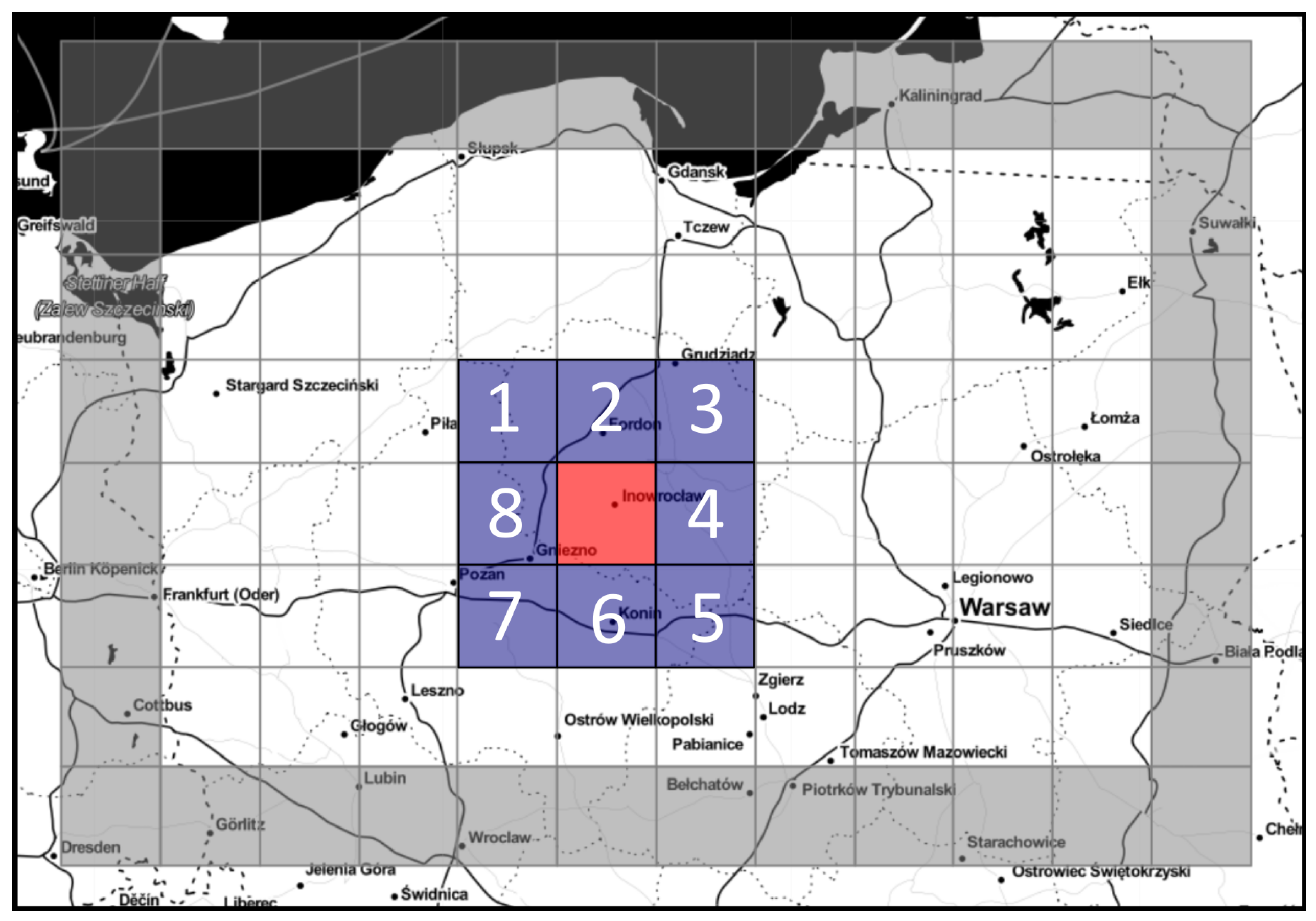
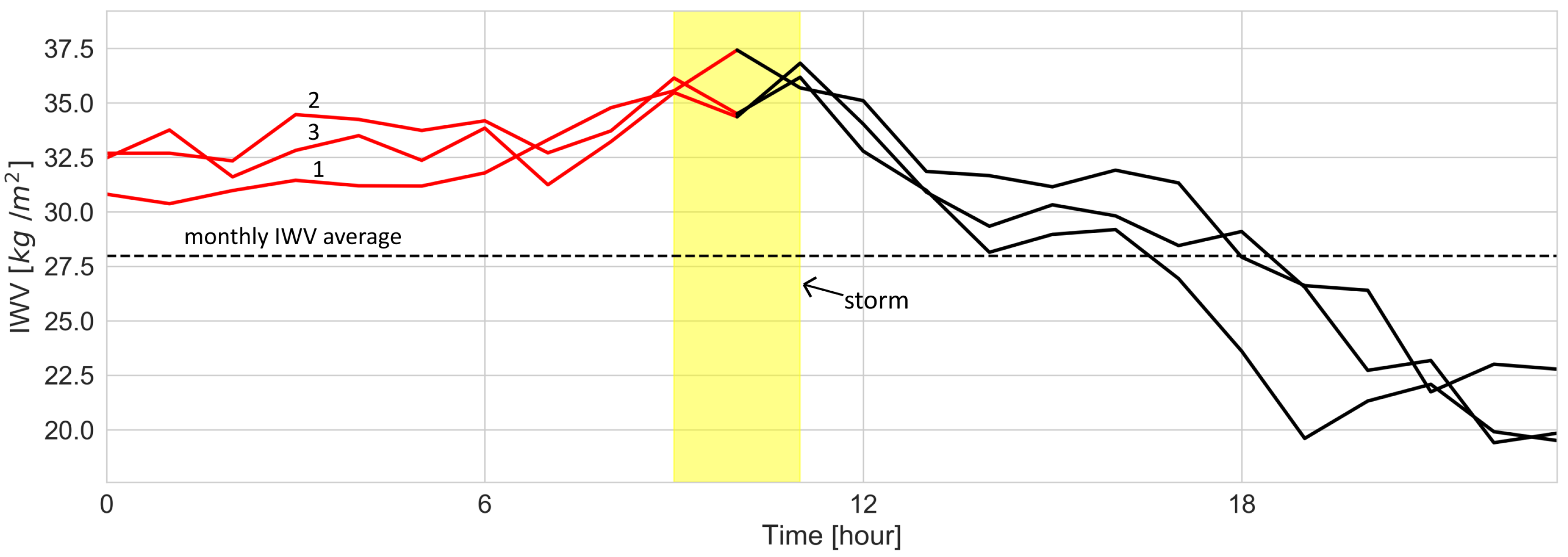
2.1.1. Integrated Water Vapour Observations

The IWV data are retrieved from the GNSS network processed routinely by WUEL processing centre in Near Real-Time mode, hosted at WUELS [29] (Zenith Troposphere Delay— Z T D G N S S ) and Weather Research and Forecasting model provided by University of Wroclaw [30] (Zenith Hydrostatic Delay— Z H D W R F ), using following equations:
I W V = Z T D G N S S Z H D W R F Q ,
where Q is a polynomial that can be expressed by the surface temperature T, mean surface temperature for the area T a and coefficients a 0 , a 1 , a 2 [31]:
Q = a 0 + a 1 T T a + a 2 T T a 2 .
The GNSS Z T D G N S S processing is based on 250 stations of ASG-EUPOS and Leica Smart Net stations, run on Berneses GNSS Software v. 5.2. Observation cut-off angle is set to 5 deg and only GPS is taken into account. Orbits and clocks are obtained from International GNSS Service (IGS) as Ultra-Rapid products, processing window is 6h, and phase ambiguity resolution is baseline length-dependent estimation (L6/L3, L1/L2, L5/L3 with SIGMA strategy, L1/L2 with Quasi Ionosphere Free (QIF) strategy) [32]. The troposphere parameters are estimated every 30 min and apriori model for troposphere (dry part only) is the Saastamoinen [33] and dry global mapping function [34]. The wet part is estimated using the Wet Global Mapping function whereas horizontal gradients mapping functions are taken from Chen et al. [35]. Zenith total delay (ZTD) is relatively constrained to 2 mm and gradients to 0.2 mm [29]. The current version of this processing (15 min latency) is now being rolled out [36]. Other components required to compute IWV are dry atmosphere parameter p and T and conversion factor Q. Both were derived from the WRF model, which is run using the following settings: model is run every 6 h and gives time series with 48 h lead time and 1-h resolution. The model domain has 48 vertical levels and a 4 × 4 km horizontal resolution [30]. Finally, dry atmosphere parameters are plugged into the following model of Saastamoinen [33]:
Z H D = 0.0022768 p 1 0.00266 cos ( 2 ϕ ) 0.00000028 H ,
where ϕ is the latitude and H is the height (orthometric). Pressure (p) and temperature (T) interpolation to the location of GNSS site is performed using method developed by [37] and tested extensively in number of studies [38,39]. These parameters are then used in the conversion factor Q (2) and hydrostatic delay Z H D determination (3).

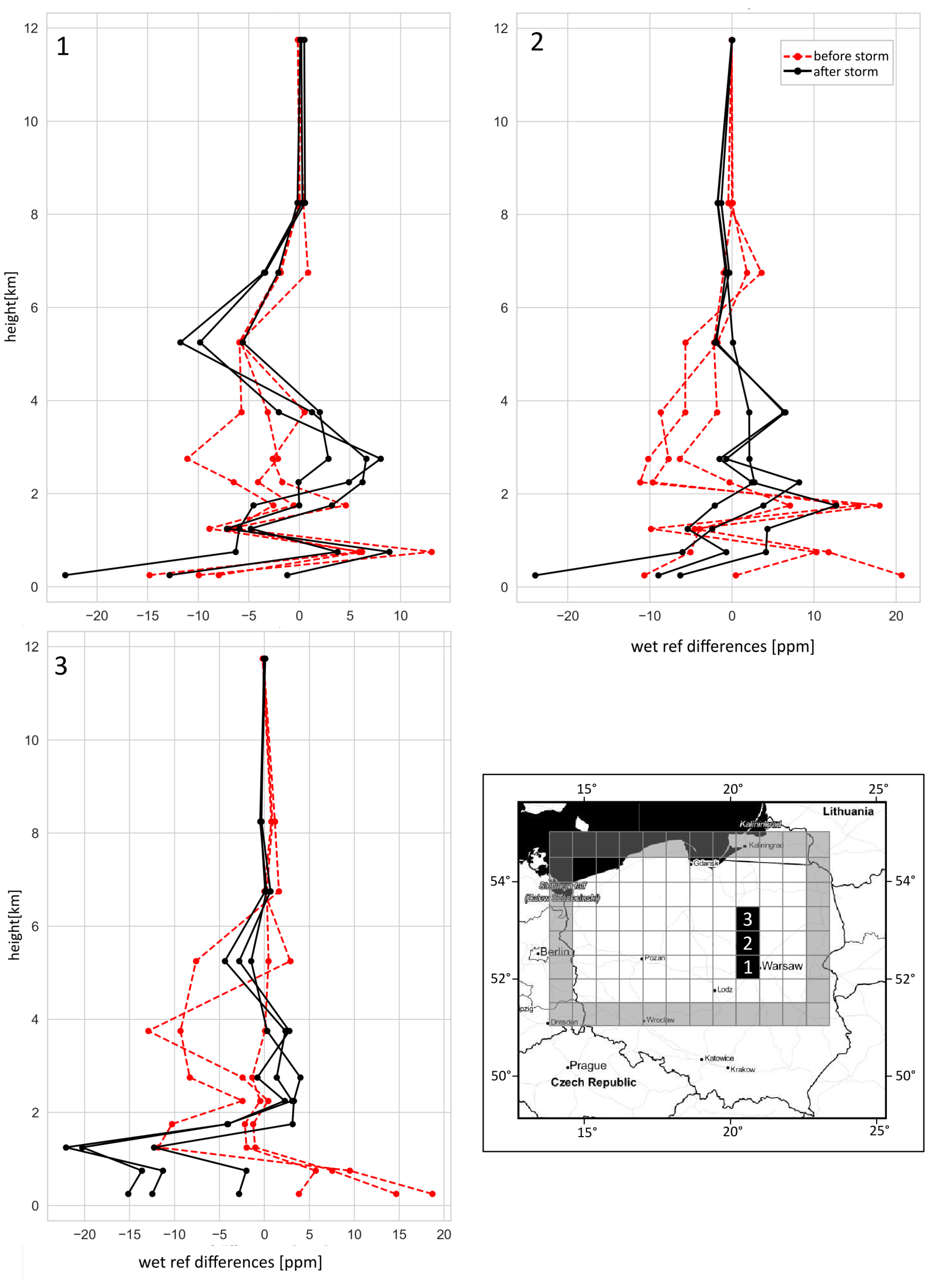
2.1.2. Wet Refractivity Data

The tomography solution applied in this study is in-house developed model TOMO2 [16,21], which is using an unconstrained robust Kalman filtering approach to solve for 3D distribution of wet refractivity. The input data are Near Real-Time operational products of UPWr E-GVAP processing centre WUELS Dymarska et al. [29]: zenith troposphere delay (ZTD), east and north gradients ( G E , G N , respectively). Data are updated every hour with a resolution of 15 min, details on troposphere processing are given in the Section 2.1.1. The observations used for wet refractivity retrieval are Slant Wet Delays (SWD) according to the following equation [15]:
S W D = m w ( e ) Z W D + G N w c o s ( ϕ ) + G E w s i n ( ϕ ) c o t ( e ) ,
where m w is a Vienna Mapping Function 1 [40] wet mapping function and G N w , G E w are wet gradients retrieved from total gradients G N , G E using method proposed by [41]. Apriori refractivity data N w apriori for all voxels are interpolated from the WRF model run by Wroclaw University [30]. The model is executed operationally 4 times a day at 00 h, 6 h, 12 h, 18 h, and forecast for the next 48 h is generated. The data for interpolation are taken from the model run closest to the analysis time, to limit the impact of a long lead-time on apriori reference field. Space interpolation of pressure p, temperature T, and water vapour e is performed using the same interpolation method as for the IWV data. Tomography system is solved following the formulation [16]:
S W D G N S S N w apriori = A G N S S A apriori · N w ,
where A G N S S consist of the path lengths of the particular GNSS rays passing through each voxel. A apriori is a binary matrix (with values of 0 or 1) depending on the presence of the additional data. N w is a matrix with wet refractivities sought for and is calculated according to the following formula:
N w . = k 2 e T + k 3 e T 2 Z w 1 .

2.1.3. Storms

We used as a storm proxy location and time of discharges from Blitzortung system [42]. The lightning location network Blitzortung was created in 2003. It consists of VLF (Very Low Frequencies) receivers spaced close to each other, separated by 50–250 km. The times of the signals are registered with microsecond precision by using a GPS receiver. The stations transmit data to a central server, where the exact positions of the discharges are computed.
Our processing was based on a GNSS tomography grid (TOMO grid), which was divided into 56 × 56 km voxels with GNSS tomography point in the centre. In order to connect discharges into the specific storms, each discharge time was compared with the previous one. If the time interval was longer than 20 min the discharge was counted as a next storm. In this way, groups of frequent discharges are created. Group of discharges was divided into ten minutes intervals. The time of the storm was determined by the highest density interval and rounded to the nearest hour.
In our classification problem, the storm activity is defined as the number of discharges per hour occurring in the voxel of GNSS tomography grid. Based on the discharges spatio-temporal density analysis, we set a threshold above 20 as the number of discharges that indicate the storm. The use of the threshold is necessary to eliminate the noise caused by the computing errors that may be falsely-located strikes and isolated discharges that do not form a storm.

2.2. Application of Random Forest Classifier

The idea of our nowcasting model was to predict a storm occurrence using refractivity and IWV information from the historical data. To perform the nowcasting task, we applied a machine learning framework—Random Forests algorithm. In order to create a storm classifier, we used the binary classification approach. The study domain was divided into 96 voxels based on the TOMO grid.

2.2.1. Input Features

The storm has not only temporal but also spatial character. The input data includes information about 3 h of refractivity data on different heights and average IWV value calculated based on the values of the nearest stations. To take into account the continuity of weather fields and potential advection, we constructed spatial features using neighbourhood information. The eight nearest voxels formed a neighbourhood for the centre box (Figure 1) and were used as additional information to the model.

2.2.2. Random Forest Classifier

Random Forest (RF) classifier is an ensemble machine learning algorithm which classifies data using decision trees. Ensemble methods allow to combine several base models in order to produce one optimal predictive model. Introduced by Breiman et al. Breiman [43], RF is a modification of the bagging technique, also called bootstrap aggregation. Bagging helps to avoid overfitting and reduces the variance of tree predictors [44]. Tree bagging samples the subsets of the dataset and fits decision trees separately to each subset creating a set of uncorrelated models. After, the result is calculated by the majority vote of trained trees. The RF method modifies the bagging process in a way that not only records are randomly selected by also their attributes are chosen on random. This way only a part of data is used for sampling. Unused examples create the out-of-bag instances (OOB) that do not participate in the training process. OOB is used to determine the best split of the randomly chosen attributes.

2.2.3. Data Preprocessing

Data preprocessing is an important part of the machine learning process. In our research, before learning part, we applied transformation techniques to improve model performance. The first step was to split data into training and testing set. To avoid overfitting, data were split by events, where three storms were left out as a testing set and the rest of the data were used for training. The splitting of the data was done at the beginning to avoid the impact of further transformations on the testing set [45]. After, we have balanced the training set. In our dataset, the number of cases without storms exceed the cases with storms. Because of this highly unbalanced characteristic of the training set, we have applied a random undersampling technique [46] by deleting examples from the majority class—where there were no discharges.

2.2.4. Implementation of Storm Classifier

The RF algorithm has a number of the modifiable hyperparameters that have an impact on the performance of the classifier. Hyperparameters have to be set up before algorithm training. To tune hyperparameters, we use a Random Search algorithm with 5-fold cross-validation applied. In n-fold cross-validation the original sample is randomly split n-times into n equal size subsamples, learning and testing sets, which are used to train and evaluate models. The n results from the folds are averaged to produce a single estimation. Random Search is a parameter tuning technique where n random combinations are selected to find the best solution for the model. The number of iterations was set to 200. In this work, we use a modification of the RF algorithm called Balanced Random Forest which uses an undersampling technique for every process of decision tree formation, that is the same number of each class representatives is selected during the bootstrapping process [47].
We tune the four most impactful parameters [48]:
  • Max depth—the maximum depth of the tree (from 1 to 11).
    Each tree in RF makes multiple splits. The depth of the tree relates to how much information is captured. Larger depth in a tree allows to explain more variation in the data. However, too many splits can cause overfitting.
  • Max features—the number of features to consider when looking for the best split (from 1 to 216).
    Before determining the best split RF model randomly resamples features. Trees with a large selection of features from which the best split is chosen might have better performance. However, when many features are considered, trees can be less diverse which will decrease their RF algorithm accuracy.
  • N estimators—the number of trees in the forest (from 10 to 2000).
    Increased number of estimators improves the accuracy of the model, but this is done at the expense of a longer learning process and might be computationally expensive.
  • Min sample leaf—the minimum number of samples required to be at a leaf node (from 1 to 21).
    The optimal value of the minimum number of samples at the leaf depends on the size of the learning set. Too large values may not be able to capture sufficient variation in the data.

2.2.5. Evaluation Metrics

To measure the strength of a classifier statistical metrics called confusion matrix is used [49]. The confusion matrix (Table 1) gives an insight into the types of errors that are being made by a classifier during testing. It comprises of four elements: true positive (TP) and true negative (TN), which refer to correctly predicted classes, and false positive (FP) and false negative (FN) which correspond to the incorrect classification.
The accuracy is a widely used evaluation metric in machine learning, either for binary or multi-class classification problems [49]. It shows the proportion of correctly classified cases out of the total amount of predicted cases:
Accuracy = TP + TN TP + FP + TN + FN
Other metrics measuring the performance of the algorithm in classifying positive cases are sensitivity and precision [50]. Sensitivity is the proportion of correctly classified positive cases out of the total amount of positive cases (Equation (8)), while precision refers to the proportion of correctly classified positive cases out of the total amount of classified positive cases (Equation (9)).
Sensitivity = TP TP + FN
Precision = TP TP + FP
Specificity and Negative Predicted Value measure the performance of the model in classifying negative cases. Specificity refers to the proportion of correctly classified cases out of the total amount of negative cases (Equation (10)). Negative Predicted Value is determined to illustrate the proportion of correctly classified negative cases out of the total amount of classified negative cases (Equation (11)).
Specificity = TN TN + FP
NPV = TN TN + FN
To measure the influence of a specific feature on the performance of the model, feature importances were computed. In RF, every node of a tree creates a condition on a single feature. The impurity is a measure based on which the optimal condition is chosen. Mean Decrease in Impurity (MDI) or Gini Importance determinates the classification impact of the features by totalling the amount of decrease in impurity as the classification is performed. A higher MDI value of the variables means that it has a greater impact on the classification.

3. Results

In this section, we demonstrate the outcomes of applying the RF classifier on storm nowcasting with only the GNSS-based input namely IWV and Wet refractivity. The classifier was tested in the area of central and northern Poland for June, July and August of 2017 and 2019. We first demonstrate the attribute selection process, which is documented by examples from 12 of August 2017. These include profiles of wet refractivity and IWV time evolution. In further steps, we present the analysis of the whole testing dataset by contingency table and feature importance characteristics.

3.1. Random Forest Classifier for Storm Nowcasting

3.1.1. Attribute Selection

In this study, variables used as an input to RF Classifier are the GNSS tomography (wet refractivity) and IWV data. The GNSS tomography data contained information about refractivity at the 11 vertical levels. Preliminary tests have shown that refractivity changes at levels below 4 km might correlate with storm occurrence. Figure 2 presents the change of wet refractivity profile 3 h before (red line) and after (black line) a randomly selected storm on 12 August 2017. As seen in the Figure 2 there are changes in the profile of wet refractivity before and after the storm in the lower part of the troposphere. In all three locations (box 1, 2 and 3) the N w in the 2–4 km height before the storm is smaller than after the storm. Moreover, the bottom part of the troposphere (0–2 km) shows high variability in N w . The relative decrease of N w content before the storm could be linked (1) to updrafts lifting the air mass above the condensation line resulting to rapid condensation in the 2–4 km height band or (2) dry air intrusion associated with atmospheric dynamics. This result shows the nowcasting potential of wet refractivity profiles up to 3 h before a storm.
Another feature reported by [13] is the distinction between daily IWV values for storms with and without thunder registrations in the period May–September 2010–2015. A monthly IWV threshold was derived for Sofia (Bulgaria). Our IWV thresholds for Poland were determined using data collected in the period June–August 2015–2019. The averages values of IWV are computed for days with (ST) and without (NST) thunderstorm. The results are presented in the Table 2.
As seen in Table 2, July and August have similar average values and they are slightly higher than the averages in June. However, for every month the differences between IWV(NST) and IWV(ST) are similar in the range of 5 kg/m 2 (22%). The IWV values during storm days (ST) are significantly higher. Thus our analysis confirmed the separation between ST and NST IWV values in Southeast Europe (Sofia, Bulgaria) reported by [13].
Further, we applied the obtained IWV threshold for an analysis of storm conditions on 12 August 2017. In Figure 2 are plotted the IWV hourly values and the calculated monthly IWV(ST) thresholds (Table 2). It is seen that 9 h ahead of a storm the hourly IWV values for each location are exceeding threshold value by at least 5 kg/m 2 . Another feature in Figure 3 is that storm occurrence is collocated with the maximum IWV value.
Using only IWV in all cells of the model, as well as full information from tomography we evaluated the mean decrease of impurity (Figure 4). The results show that the most important features to the forecast are these related to the voxels northward and westward (n7, n2, n3 and n1) to the predicted one. Namely the first three parameters are: Nw1.75_n7_1h, Nw2.25_n2_1h, Nw2.25_n2_2h, (see Figure 1). Moreover, Nw has a dominant role in nowcasting. The first 5 parameters are linked with the tomography (Figure 4) and levels with visible differences between onset and storm dissipation (Figure 2). The IWV data are also important but only in the west (IWV_n8_1h and IWV_n1_2h) of the storm.

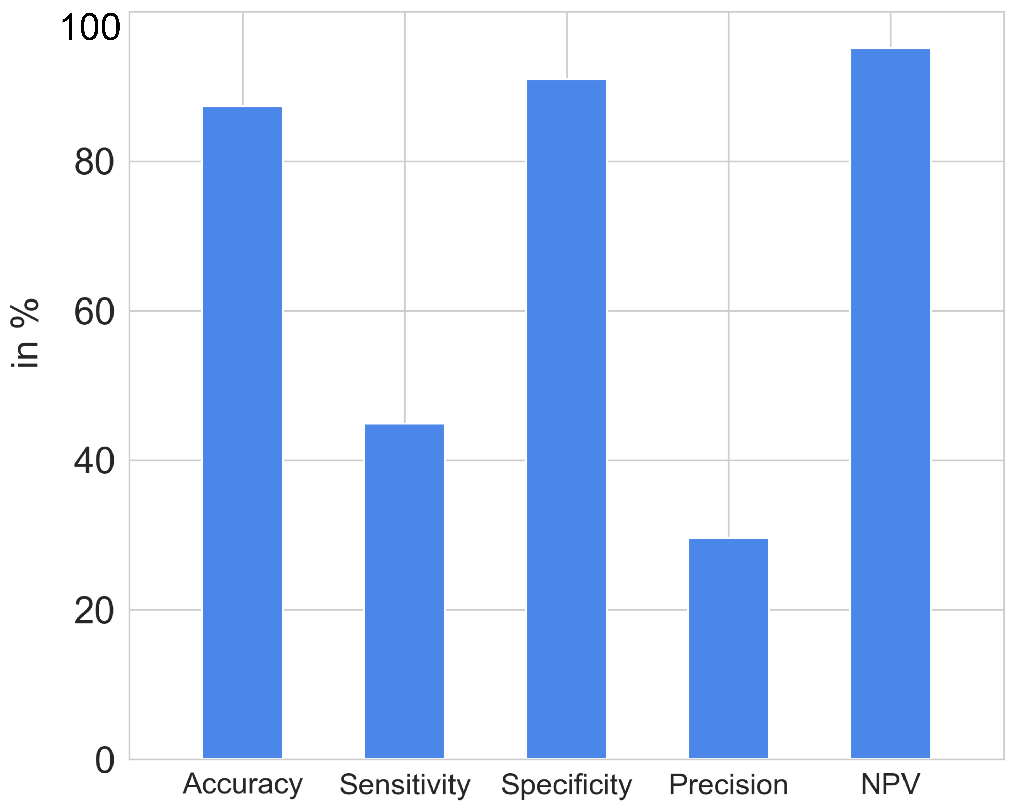
3.1.2. Classifier Performance
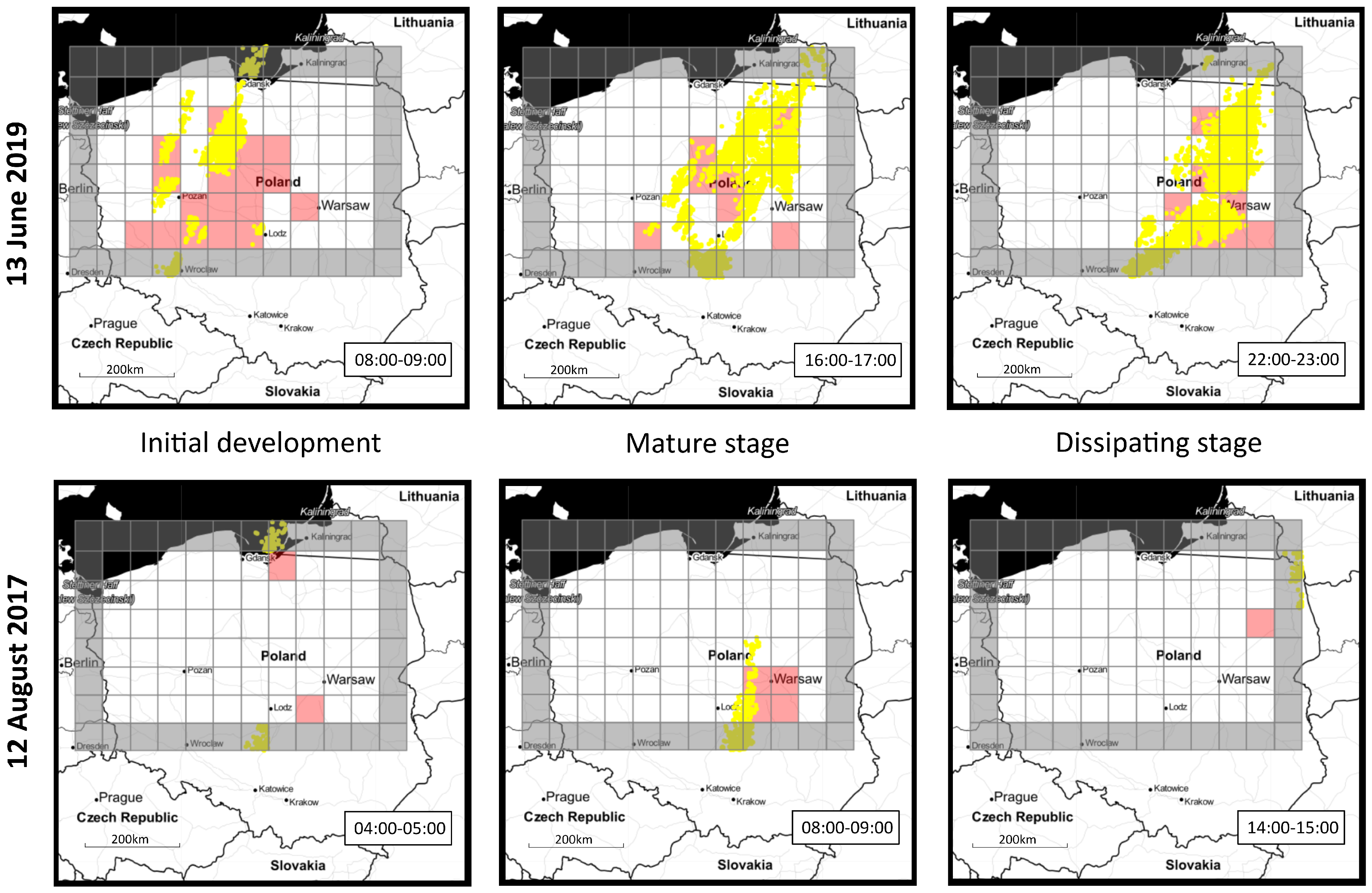
The classifier performance was tested on a data sample which includes 493 h of storm cases and 3664 cases without a storm. To assess the classification of the testing set we used the confusion matrix (Table 3). The matrix shows a classification result, where the diagonal positions represent the number of correctly classified cases.
Presented in Figure 5 are the metrics determined using the confusion matrix namely: Accuracy, Sensitivity, Specificity, Precision and Negative Predicted Value (NPV). The Accuracy of a storm classifier informs about the proportion of correctly predicted cases (storm and no storm) among all cases. With a value 87.35% it is high, but in the case of imbalanced data, it is not a sufficient measure. To have a better view of the classifier performance we need to calculate additional metrics. Sensitivity, which is the number of correctly predicted storms over the number of all real storms cases, shows an average value over 44%. It means that the algorithm captures storm occurrences, missing 347 cases from 493. Specificity reaches over 90%. It presents the proportion of correct predictions of no storms out of the total amount of all predicted no storms cases. The worst result (less than 30%) is for Precision. The low value of this measure means that the algorithm predicts storm occurrence in voxels where in reality there is no storm. The NPV has the highest value reaching 95% and it shows that model has good result in predicting no storm cases. NPV is measured to determine the proportion of correctly predicted no storm cases and the total amount of real no storm cases.

3.1.3. Case Studies

Figure 6 presents visualisation for two case studies of storm event for 13 June 2019 (top row) and 12 August 2017 (bottom row). The maps show observed lightning activities (yellow dots) and the result of predicted storm localisation indicated by the red colour for three stages of the storm: initial development, mature and dissipating.
On 13 June 2019 storm with the substantial number of discharges developed over Poland. Predictions for the beginning of the storm observed between 8 and 9 UTC are overestimated, the algorithm forecast a larger area of the storm occurrence than it actually was. However, the majority of the areas affected were captured. For the mature and dissipating stage clearly seen is that prediction indicates correct areas of the discharges, however, it misses the part of the storm. 12 August 2017 is an example of a minor storm recorded in Poland. For the initial development between 4 and 5 UTC and also for dissipating stage between 14 and 15 UTC, the discharges were registered at the border of the studied area. The predictions for these stages are located very close to discharges. The approximate location of storm mature stage in August between 8:00 and 9:00 UTC is predicted well, however, it misses one voxel with discharges and extends the storm to the east by 2 additional locations.
As seen in a Table 4, the number of “No Storm” is prevailing in the data set. The “Storm” locations are: in the 1st of August 2017 case just 71, in the 12th of August 2017 case just 47 and the major storm of 13th of June 2019 375. It is clear that the model is predicting well the smaller storms (see the second row of Figure 6), while the larger events such as the one from 13th of June 2019 is not. The major problem is linked with not predicting enough storm locations (only 72 hits out of 375) for such extended storm.

4. Discussion

Due to the potential of large economic losses caused by severe weather, storm nowcasting is an important challenge in the operational forecasting. Previous cornerstone study by [7] made extensive use of IWV to predict the rainfall intensity in Portugal, stating that the most rainfall will occur in the rapidly descending part of the IWV broken line approximation of trend line. In our study for Poland, we observed the most intense thunder activity in the tip of an ascending ramp of IWV (Figure 3). However, we did not find that the most intense rainfall is connected with dense discharges activities. Therefore, our results follow a similar pattern but are not exactly similar. This can be explained by the different geographic location and predominant atmospheric circulation. In the study by [13] in Bulgaria, IWV threshold for a day with a storm was used to discriminate days with a large potential to develop storms. We used this finding but we applied it to a short term (0–2 h) storm predictor. Our results presented in Figure 4, confirm a high importance of Nw factor. A closer inspection of the feature importance (Figure 4) reveals that the Nw has a dominant impact on the performance of our RF classifier. The most prominent features are Nw 2 and 1 h ahead of a storm occurrence and a grid number 7 and 2 (westerly advection direction). Less important, but still at the top of the list, are IWV from grid 8 and 1 which also are to the west of the grid.
A study by Benevides et al. [9] on the use of GNSS for severe weather nowcasting, used machine learning methods. Except for the IWV, they have added the pressure, temperature, relative humidity, cloud top temperature, cloud top pressure and cloud top height to the input data. The study reported upgraded Accuracy and the lowered number of false positive classified cases. However, only one station was used for testing. In our study, we use a machine learning approach, adding the wet 3D refractivity observations (as advised by [7]) and applying a simpler machine learning algorithm (Random Forest). The advantage of Random Forest is an easy connection to the physics of the atmosphere through the choice of parameters: (1) IWV above or below the threshold for storm or no storm day, (2) wet refractivity in voxels around the predicted storm location to take into account horizontal dynamics, (3) use of multiple layers of tomography to identify convection dynamics, (4) the evolution of these parameters in time.
Based on the feature importance (Figure 4) we conclude that wet refractivity below 7 km is useful in predicting storm location, with layers at height of 2.25 km and 1.75 km being at the top of the feature importance list. This is further confirmed in Figure 2, where the majority of the difference between pre-storm and post-storm refractivity is visible in the 2–4 km height.
The accuracy of the prediction model reaches over 87%. Although the high result in Accuracy, the model has some limitation. The problem of the classifier is a large number of false alarms, something that was also reported by [7]. Therefore, in future studies, we will consider other factors, such as instability indexes [13]. Moreover increasing training set can improve prediction results. It should be noted that in [23], where Precision was around 50%, false alarms were often found behind or at the location of old storms. However, in that study predictions were made for voxel size 0.06 × 0.06 × 20 levels (translates to roughly 5 × 5 km and 20 levels) for 30 min, therefore the granularity of this study was much higher compared to our 0–2 h lead time and voxel size 56 × 56 km. Another limitation of the model is Sensitivity reaching 44%. It means that more than half of the storms are not detected. However, an inspection of the case studies (Figure 6) shows that, despite the low results in Precision and Sensitivity, the model can find the approximate location of the storm. For the initial stage of the storm on 13 June 2019, the majority of the predicted locations overlap with the registered thunderstorms. The predictions extend the storm with 10 additional voxels which results in a large number of false alarms. The reason for this may be the detection of favourable conditions for the formation of a storm cloud. Adding information about the clouds could improve the accuracy of the predictions. On 12 August 2017 at an initial and dissipating stage, the false alarms also occur. The forecasts between 4 and 5 UTC are close to an impending storm that will occur at this location in the next hour, while the false alarm for dissipating stage is found at the location of an old storm. The modification of the temporal resolution could improve Precision of the model.
Not only the choice of parameters should be extended in future application of our methodology. We also think that a denser GNSS network of 5–10 km inter-station distance will help to build more reliable tomography models, especially in the lower atmosphere [14]. Moreover, it can resolve the vertical dynamics of the troposphere as observing scales would be closer to the size of predicted features [51].
This work confirms and advances the finding obtained with the GNSS tropospheric products in Southwest and Southeast Europe (Portugal and Bulgaria). Of particular significance for nowcasting application in Poland are the obtained IWV thresholds for the summer storm season June-July-August and the vertical profiles of wet refractivity. The 2–3 h predictive capabilities of GNSS derived products are of particular interest for the operational service developed in Southeast Europe targeting application in severe weather and hail suppression in Bulgaria in particular [52].

5. Conclusions

In this article, a combined IWV and tomography-based wet refractivity profiles are used in a machine learning framework to predict summer storms occurrence in Poland. Random Forest classifier is trained on data covering the period from June to August 2017 and 2019. The results show that the most important features are these related to the voxels westward to the storm location, with the first parameters being: (1) wet refractivity at height 1.75 km, (2) wet refractivity at the height 2.25 km, (3) same voxel but 1 h before. IWV is found to have a major contribution with 3 out of 8 most influential features obtained by the machine learning. Storm classifier performance is tested on three data samples, discussed in Section 3.1.3. The classifier accuracy is above 84%. However, the precision of classification shows that the model overestimates the number of storm occurrence, reaching less than 30%. IWV thresholds for Poland are determined using data collected in the period June–August 2015–2019. The monthly IWV value for storm cases is found to be 22% higher than the IWV for a case without a storm. A randomly selected storm case analysis demonstrates that there is a difference between pre-storm and post-storm refractivity profile on levels below 6 km.

Author Contributions

Conceptualization, W.R. and G.G.; methodology, K.S., W.R and M.Ł.; software, M.Ł. and W.R.; validation, M.Ł. and G.G.; formal analysis, K.S. and G.G.; investigation, M.Ł.; resources, M.Ł.; data curation, M.Ł.; writing–original draft preparation, M.Ł.; writing–review and editing, G.G., W.R. and K.S.; visualization, M.Ł.; supervision, W.R.; project administration, W.R.; funding acquisition, W.R. All authors have read and agree to the published version of the manuscript.

Funding

This research was funded by National Science Centre grant number UMO-2015/17/B/ST10/03827, MATLAB Software License No. 101979.

Acknowledgments

We are grateful to the University of Wroclaw and Maciej Kryza for the provision of WRF data for TOMO2 model apriori, we are also thankful to blitzortung.org for providing reference data.

Conflicts of Interest

The authors declare no conflict of interest.

Abbreviations

The following abbreviations are used in this manuscript:
GNSSGlobal Navigation Satellite Systems
GPSGlobal Positioning System
PWVPrecipitable Water Vapour
IWVIntegrated Water Vapour
ZTDZenith Troposphere Delay
WRFWeather Research and Forecasting
E-GVAPThe EUMETNET EIG GNSS water vapour programme
NPVNegative Predicted Value
MDIMean Decrease in Impurity
UPWrWroclaw University of Environmental and Life Sciences

References

  1. Wang, Y.; Coning, E.; Harou, A.; Jacobs, W.; Joe, P.; Nikitina, L.; Roberts, R.; Wang, J.; Wilson, J.; Atencia, A.; et al. Guidelines for Nowcasting Techniques; Number 1198; World Meteorological Organization (WMO): Geneva, Switzerland, 2017. [Google Scholar]
  2. Shi, X.; Chen, Z.; Wang, H.; Yeung, D.Y.; Wong, W.k.; Woo, W.c. Convolutional LSTM Network: A Machine Learning Approach for Precipitation Nowcasting. Adv. Neural Inf. Process. Syst. 2015, 2015, 802–810. [Google Scholar]
  3. Browning, K.A.; Collier, C.G. Nowcasting of precipitation systems. Rev. Geophys. 1989, 27, 345–370. [Google Scholar] [CrossRef]
  4. Guerova, G.; Jones, J.; Douša, J.; Dick, G.; de Haan, S.; Pottiaux, E.; Bock, O.; Pacione, R.; Elgered, G.; Vedel, H.; et al. Review of the state of the art and future prospects of the ground-based GNSS meteorology in Europe. Atmos. Meas. Tech. 2016, 9, 5385–5406. [Google Scholar] [CrossRef] [Green Version]
  5. Douša, J.; Dick, G.; Kačmařík, M.; Bro Řková, R.; Zus, F.; Brenot, H.; Stoycheva, A.; Möller, G.; Kaplon, J. Benchmark campaign and case study episode in central Europe for development and assessment of advanced GNSS tropospheric models and products. Atmos. Meas. Tech. 2016, 9, 2989–3008. [Google Scholar] [CrossRef] [Green Version]
  6. Václavovic, P.; Douša, J.; Teferle, F. GNSS Real-Time PPP Demonstration Campaign; Springer: Cham, Switzerland, 2020; pp. 45–48. [Google Scholar] [CrossRef]
  7. Benevides, P.; Catalao, J.; Miranda, P.M.A. On the inclusion of GPS precipitable water vapour in the nowcasting of rainfall. Nat. Hazards Earth Syst. Sci. 2015, 15, 2605–2616. [Google Scholar] [CrossRef] [Green Version]
  8. Yao, Y.; Shan, L.; Zhao, Q. Establishing a method of short-term rainfall forecasting based on GNSS-derived PWV and its application. Sci. Rep. 2017, 7, 12465. [Google Scholar] [CrossRef]
  9. Benevides, P.; Catalao, J.; Nico, G. Neural Network Approach to Forecast Hourly Intense Rainfall Using GNSS Precipitable Water Vapor and Meteorological Sensors. Remote Sens. 2019, 11, 966. [Google Scholar] [CrossRef] [Green Version]
  10. Wilson, J.W.; Crook, N.A.; Mueller, C.K.; Sun, J.; Dixon, M. Nowcasting Thunderstorms: A Status Report. Bull. Am. Meteorol. Soc. 1998, 79, 2079–2099. [Google Scholar] [CrossRef]
  11. Cooper, M.A.; Holle, R.L. Reducing Lightning Injuries Worldwide; Springer: Cham, Switzerland, 2019; Number June; pp. 153–160. [Google Scholar] [CrossRef]
  12. Suparta, W.; Adnan, J.; Mohd Ali, M.A. Nowcasting the lightning activity in Peninsular Malaysia using the GPS PWV during the 2009 inter-monsoons. Ann. Geophys. 2014, 57, 1–13. [Google Scholar] [CrossRef]
  13. Guerova, G.; Dimitrova, T.; Georgiev, S. Thunderstorm Classification Functions Based on Instability Indices and GNSS IWV for the Sofia Plain. Remote Sens. 2019, 11, 2988. [Google Scholar] [CrossRef] [Green Version]
  14. Brenot, H.; Rohm, W.; Kačmařík, M.; Möller, G.; Sá, A.; Tondaś, D.; Rapant, L.; Biondi, R.; Manning, T.; Champollion, C. Cross-Comparison and methodological improvement in GPS tomography. Remote Sens. 2020, 12, 30. [Google Scholar] [CrossRef] [Green Version]
  15. Flores, A.; Ruffini, G.; Rius, A. 4D tropospheric tomography using GPS slant wet delays. Ann. Geophys. 2000. [Google Scholar] [CrossRef]
  16. Rohm, W.; Zhang, K.; Bosy, J. Limited constraint, robust Kalman filtering for GNSS troposphere tomography. Atmos. Meas. Tech. 2014. [Google Scholar] [CrossRef] [Green Version]
  17. Kak, A.C.; Slaney, M.; Wang, G. Principles of Computerized Tomographic Imaging. Med. Phys. 2002. [Google Scholar] [CrossRef]
  18. Manning, T.; Rohm, W.; Zhang, K.; Hurter, F.; Wang, C. Determining the 4D dynamics of wet refractivity using GPS tomography in the Australian region. In Proceedings of the IAG General Assembly, Melbourne, Australia, 28 June–2 July 2011. [Google Scholar] [CrossRef]
  19. Zhang, K.; Manning, T.; Wu, S.; Rohm, W.; Silcock, D.; Choy, S. Capturing the Signature of Severe Weather Events in Australia Using GPS Measurements. IEEE J. Sel. Top. Appl. Earth Obs. Remote Sens. 2015. [Google Scholar] [CrossRef]
  20. Jiang, P.; Ye, S.R.; Liu, Y.Y.; Zhang, J.J.; Xia, P.F. Near real-time water vapor tomography using ground-based GPS and meteorological data: Long-term experiment in Hong Kong. Ann. Geophys. 2014. [Google Scholar] [CrossRef] [Green Version]
  21. Trzcina, E.; Rohm, W. Estimation of 3D wet refractivity by tomography, combining GNSS and NWP data: First results from assimilation of wet refractivity into NWP. Q. J. R. Meteorol. Soc. 2019. [Google Scholar] [CrossRef]
  22. Hanna, N.; Trzcina, E.; Möller, G.; Rohm, W.; Weber, R. Assimilation of GNSS tomography products into the Weather Research and Forecasting model using radio occultation data assimilation operator. Atmos. Meas. Tech. 2019. [Google Scholar] [CrossRef]
  23. Han, L.; Sun, J.; Zhang, W.; Xiu, Y.; Feng, H.; Lin, Y. A machine learning nowcasting method based on real-time reanalysis data. J. Geophys. Res. Atmos. 2017, 122, 4038–4051. [Google Scholar] [CrossRef]
  24. Zhang, W.; Han, L.; Sun, J.; Guo, H.; Dai, J. Application of Multi-channel 3D-cube Successive Convolution Network for Convective Storm Nowcasting. In Proceedings of the 2019 IEEE International Conference on Big Data (Big Data), Los Angeles, CA, USA, 9–12 December 2019; pp. 1705–1710. [Google Scholar] [CrossRef] [Green Version]
  25. Veillette, M.S.; Iskenderian, H.; Lamey, P.M.; Bickmeier, L.J. Convective Initiation Forecasts Through the Use of Machine Learning Methods. In Proceedings of the 16th Conference on Aviation, Range, and Aerospace Meteorology, Austin, TX, USA, 9 January 2013; American Meteorological Society: Boston, MA, USA, 2013. [Google Scholar]
  26. Ruiz, A.; Villa, N. Storms prediction: Logistic regression vs random forest for unbalanced data. Case Stud. Bus. Ind. Gov. Stat. 2007, 1, 91–101. [Google Scholar]
  27. Williams, J.K.; Ahijevych, D.; Dettling, S.; Steiner, M. Combining observations and model data for short-term storm forecasting. In Remote Sensing Applications for Aviation Weather Hazard Detection and Decision Support; Feltz, W.F., Murray, J.J., Eds.; Proc. SPIE: San Diego, CA, USA, 2008; Volume 7088, p. 708805. [Google Scholar] [CrossRef]
  28. Ahijevych, D.; Pinto, J.O.; Williams, J.K.; Steiner, M. Probabilistic Forecasts of Mesoscale Convective System Initiation Using the Random Forest Data Mining Technique. Weather Forecast. 2016, 31, 581–599. [Google Scholar] [CrossRef]
  29. Dymarska, N.; Rohm, W.; Sierny, J.; Kapłon, J.; Kubik, T.; Kryza, M.; Jutarski, J.; Gierczak, J.; Kosierb, R. An assessment of the quality of near-real time GNSS observations as a potential data source for meteorology. Meteorol. Hydrol. Water Manag. 2017, 5, 3–13. [Google Scholar] [CrossRef]
  30. Kryza, M.; Werner, M.; Wałszek, K.; Dore, A.J. Application and evaluation of the WRF model for high-resolution forecasting of rainfall—A case study of SW Poland. Meteorol. Z. 2013, 22, 595–601. [Google Scholar] [CrossRef]
  31. Emardson, T.R. The systematic behavior of water vapor estimates using four years of GPS observations. IEEE Trans. Geosci. Remote Sens. 2000. [Google Scholar] [CrossRef]
  32. Dach, R.; Lutz, S.; Walser, P.; Fridez, P. Bernese GNSS software version 5.2. 2015. [Google Scholar]
  33. Saastamoinen, J. Contributions to the theory of atmospheric refraction. Bull. Géodésique 1972, 105, 279–298. [Google Scholar] [CrossRef]
  34. Boehm, J.; Niell, A.; Tregoning, P.; Schuh, H. Global Mapping Function (GMF): A new empirical mapping function based on numerical weather model data. Geophys. Res. Lett. 2006, 33, L07304. [Google Scholar] [CrossRef] [Green Version]
  35. Chen, G.; Herring, T.A. Effects of atmospheric azimuthal asymmetry on the analysis of space geodetic data. J. Geophys. Res. Solid Earth 1997, 102, 20489–20502. [Google Scholar] [CrossRef]
  36. Tondaś, D.; Kapłon, J.; Rohm, W. Ultra-fast near real-time estimation of troposphere parameters and coordinates from GPS data. Measurement 2020, 162, 107849. [Google Scholar] [CrossRef]
  37. Karabatić, A.; Weber, R.; Haiden, T. Near real-time estimation of tropospheric water vapour content from ground based GNSS data and its potential contribution to weather now-casting in Austria. Adv. Space Res. 2011, 47, 1691–1703. [Google Scholar] [CrossRef]
  38. Bosy, J.; Kaplon, J.; Rohm, W.; Sierny, J.; Hadas, T. Near real-time estimation of water vapour in the troposphere using ground GNSS and the meteorological data. Ann. Geophys. 2012, 30. [Google Scholar] [CrossRef] [Green Version]
  39. Wilgan, K.; Rohm, W.; Bosy, J. Multi-observation meteorological and GNSS data comparison with Numerical Weather Prediction model. Atmos. Res. 2015, 156, 29–42. [Google Scholar] [CrossRef]
  40. Boehm, J.; Kouba, J.; Schuh, H. Forecast Vienna mapping functions 1 for real-time analysis of space geodetic observations. J. Geod. 2009. [Google Scholar] [CrossRef]
  41. Shoji, Y. Retrieval of water vapor inhomogeneity using the japanese nationwide GPS array and its potential for prediction of convective precipitation. J. Meteorol. Soc. Jpn. 2013. [Google Scholar] [CrossRef] [Green Version]
  42. Wanke, E.; Andersen, R.; Volgnandt, T. A World-Wide Low-Cost Community-Based Time-of-Arrival Lightning Detection and Lightning Location Network 2014. pp. 1–95. Available online: www.blitzortung.org/Documents/TOA_Blitzortung_RED.pdf (accessed on 18 April 2020).
  43. Breiman, L. Random forests. Mach. Learn. 2001, 45, 5–32. [Google Scholar] [CrossRef] [Green Version]
  44. Breiman, L. Bagging predictors. Mach. Learn. 1996, 24, 123–140. [Google Scholar] [CrossRef] [Green Version]
  45. Geron, A. Hands-on Machine Learning With Scikit-Learn and TensorFlow: Concepts, Tools, and Techniques to Build Intelligent Systems; O’Reilly Media: Sebastopol, CA, USA, 2017. [Google Scholar]
  46. More, A. Survey of resampling techniques for improving classification performance in unbalanced datasets. arXiv 2016, arXiv:1608.06048. [Google Scholar]
  47. Chen, C.; Liaw, A.; Breiman, L. Using Random Forest to Learn Imbalanced Data; University of California, Berkeley: Berkeley, CA, USA, 2004; Volume 110, pp. 1–12. [Google Scholar]
  48. Pedregosa, F.; Varoquaux, G.; Gramfort, A.; Michel, V.; Thirion, B.; Grisel, O.; Blondel, M.; Prettenhofer, P.; Weiss, R.; Dubourg, V.; et al. Scikit-learn: Machine Learning in Python. J. Mach. Learn. Res. 2012, 12, 2825–2830. [Google Scholar]
  49. Hossin, M.; Sulaiman, M.N. A Review on Evaluation Metrics for Data Classification Evaluations. Int. J. Data Min. Knowl. Manag. Process 2015, 5, 1–11. [Google Scholar] [CrossRef]
  50. Powers, D.M.W. Evaluation: From precision, recall and F-measure to ROC, informedness, markedness and correlation. J. Mach. Learn. Technol. 2011, 2, 37–63. [Google Scholar]
  51. Houze, R.A. Mesoscale convective systems. Rev. Geophys. 2004, 42, RG4003. [Google Scholar] [CrossRef] [Green Version]
  52. Guerova, G.; Dimitrova, T.; Vassileva, K.; Slavchev, M.; Stoev, K.; Georgiev, S. BalkanMed real time severe weather service: progress and prospects in Bulgaria. Adv. Space Res. 2020. [Google Scholar] [CrossRef]
Figure 1. Storm nowcasting area. The input data contains the 3 previous hours of GNSS tomography and IWV data from the prediction area (red box) and the neighbourhood (blue boxes). Grey boxes are excluded from the predictions, however, they are taken into account as the neighbourhood.
Remotesensing 12 02536 g001
Figure 2. Vertical profiles of N w change before (red dashed lines) and after (black solid lines) the storm on 12 August 2017. The map shows the location of profiles 1, 2, and 3.
Remotesensing 12 02536 g002
Figure 3. Time series of IWV values for 3 analyzed points (blue line) and storm occurrence (yellow bars) for 12 August 2017. The monthly IWV(ST) threshold is indicated as a dashed black line. The line numbering refers to the locations presented on the map in Figure 2.
Remotesensing 12 02536 g003
Figure 4. Mean decrease in impurity for the most influential features. Feature names on the chart are created as follows. The first part defines the type of data: I W V or N w . For tomography data the level is also given, the number before ‘n’ indicates a neighbour (as in Figure 1), while ‘0’ means the central voxel. The last part with ‘h’ indicates the number of hours before the prediction.
Remotesensing 12 02536 g004
Figure 5. Performance measures: Accuracy, Sensitivity, Specificity, Precision, Negative Predicted Value.
Remotesensing 12 02536 g005
Figure 6. Storm predictions for 13 June 2019 and 12 August 2017. Observed discharges are indicated by the yellow dots. The red voxels show storm predictions.
Remotesensing 12 02536 g006
Table 1. Confusion matrix for binary classification.
Actual Positive ClassActual Negative Class
Predicted Positive ClassTrue positive (TP)False positive (FP)
Predicted Negative ClassFalse negative (FN)True negative (TN)
Table 2. Monthly IWV averages for the days with a storm (ST) and without a storm (NST).
MonthIWV(NST) [ kg / m 2 ] IWV(ST) [ kg / m 2 ]
June20.4025.67
July23.0028.92
August22.7927.98
Table 3. Confusion matrix of reported and predicted storm and no storm case. The values show the number of observation.
ClassReported ‘Storm’Reported ‘No Storm’
Predicted ‘Storm’146179
Predicted ‘No storm’3473485
Table 4. Confusion matrix of reported and predicted storm and no storm case for three case studies.
DateReported ‘Storm’Reported ‘No Storm’Class
1 August 2017396Predicted ‘Storm’
32432Predicted ‘No storm’
12 August 20173562Predicted ‘Storm’
121645Predicted ‘No storm’
13 June 201972111Predicted ‘Storm’
3031408Predicted ‘No storm’

