Preliminary Selection and Characterization of Pseudo-Invariant Calibration Sites in Northwest China

Abstract

Pseudo-invariant calibration sites (PICS) have been used for the radiometric calibration and stability monitoring of satellite optical sensors. Several stable PICS, such as those in the Sahara Desert in North Africa, were selected for the vicarious calibration of earth remote sensing satellites. However, the selection procedure of PICSs in the whole of Northwest China has not been fully explored before. This paper presents a novel technique for selecting PICS in Northwest China by combined using the coefficient of variation (CV) and the iteratively reweighted multivariate alteration detection (IR-MAD) technique. IR-MAD, which calculates the differences between two multispectral N-band images from the same scene acquired at different times, is used to identify no-change pixels (NCPs) of the scene through one image pair. The NCPs from IR-MAD using the long-term data of FY-3 visible infrared radiometer (VIRR) and aqua Moderate Resolution Imaging Spectroradiometer (MODIS) were aggregated into the contiguously stable sites. The traditional spatial uniformity and temporal stability from MODIS surface products were used to select the potential PICS. By combining the results of both methods, over thirty PICSs with a wider brightness range of the scene types were selected. To confirm and characterize these PICSs over Northwest China, Landsat operational land imager (OLI) high-spatial-resolution images were used to check the spatial uniformity of the selected site to determine the specific location and the size of these sites. Additionally, the surface spectral reflectance and bidirectional reflectance distribution function (BRDF) were obtained from the field campaign at Chaidamu Basin, 2018. To demonstrate the practical utilization and usability of these PICSs, they were employed in the multi-site top of atmosphere (TOA) reflectance simulation to validate the operational calibration performance of Aqua/MODIS and FY-3D/MERSI-II (Medium Resolution Spectral Imager II). The simulation results showed good consistency compared with the observations from both MODIS and MERSI-II, with a relative bias and root mean square error (RMSE) of <5% and <0.05%, respectively. These sites provide prospects for multi-site vicarious calibrations of solar reflective bands, which may help to evaluate or characterize instrumental nonlinear responses using a wider signal dynamic from the sites in different seasons.

1. Introduction

The on-orbit calibration of space-borne earth observation instruments is required for accurate remote sensing of Earth’s environmental parameters. These instruments are not fully calibrated during the prelaunch period, and their performance is subjected to change when launched into space. Therefore, routine post-launch calibration is often required, owing to changes in environmental conditions, as well as many other factors [1,2]. To calibrate the solar reflective bands (RSB, 400–2500 nm), onboard calibration resources are often necessary; however, this increases the cost of the sensor design. Thus, vicarious calibration techniques based on the surface stable sites have been developed to independently evaluate sensor performance, which can achieve a sound accuracy of less than 5% [3,4].

Pseudo-invariant calibration sites (PICSs) on earth with specific characteristics have served as the benchmark or reference sites to verify the inflight radiometric calibration performance of satellite optical sensors. PICSs are spatially uniform, have barely changed over time, and are often located in arid regions with little rainfall or vegetation [5,6]. Additional qualifications for PICS include minimal cloud cover, low aerosol, and high elevations, where the atmosphere has minimal impact. Generally, these regions include those with sparse human activity. These test sites have been, and will continue to be, central to the calibration of earth-observing systems and the quality assurance and control (QA/QC) framework of their derived products for Earth observation [7]. Cosnefry et al. selected 20 dry desert sites located in North Africa and the Middle East, where a size of 10⁴ km² exhibits approximately 3% of the spatial nonuniformity and 1–2% of the temporal variability from the multi-temporal series of the Meteostat-4 data [8]. The Committee on Earth Observation Satellites (CEOS) endorsed six of these North-African and Middle-Eastern as standard reference sites for the post-launch calibration of space-based optical imaging sensors. These sites are Libya 4, Mauritania 1, Mauritania 2, Algeria 3, Libya 1, and Algeria 5, which have 3% or less spatial variability, in addition to 3% or less of temporal variability across all RSBs. Using five Landsat images from 1984 to 2011, Helder et al. developed an algorithm for locating optimal sites that are spatially and temporally stable [9]. This includes Libya 4, Libya 1, and Algeria 3 from the CEOS list, and new sites in Egypt and Libya 4 were also identified as the most temporally stable Saharan PICS. Shrestha et al. presented an automated method to classify North Africa for its potential use as an extended PICS (EPICS) that covers a vast portion of the African continent [10]. An automated classification algorithm was used to detect 19 “clusters” that represent distinct land surface types, and the three clusters were identified using spatial uncertainties: approximately 5% for the blue bands and 3% for the near infrared bands. The main advantage of this cluster approach is that many pixels are aggregated into a contiguously homogeneous region that can be sufficiently distributed across the continents. This allows for multiple imaging opportunities in a place of typical PICS imaging and, therefore, increases the temporal resolution to aid in quicker identification of changes in sensor responses.

PICS-based calibration is only valid if the sites exhibit reasonable spatial, temporal, and spectral stability. These desert sites are commonly used to monitor the radiometric trends of satellite instruments (e.g., Satellite Pour l’Observation de la Terre (SPOT), POLarization and Directionality of the Earth’s Reflectances (POLDER), Moderate Resolution Imaging Spectroradiometer (MODIS), The Along Track Scanning Radiometers 2 (ATSR-2), Medium Resolution Spectral Imager (MERSI), etc.) [1,11,12]. Single or multiple PICSs have demonstrated excellent potential for the absolute calibration of several sensors, including Enhanced Thematic Mapper Plus(ETM+), MODIS, UK-Disaster Monitoring Constellation (UK-DMC), MERSI, the Operational Land Imager (OLI), and the Sentinel-2A Multi-Spectral Instrument (MSI), which use an empirical absolute calibration model [13,14]. Govaerts et al. initially developed an absolute calibration model using PICS with geostationary satellites [15,16]. Bhatt et al. developed a typical PICS desert daily exoatmospheric radiance model based on a well-calibrated (reference) geostationary Earth orbit satellite visible sensor [17]. Several researchers used PICS to cross-calibrate the Sentinel-2A MSI to the OLI and estimated the agreement between the corresponding bands and achieved an approximately 1% or better of calibration accuracy [18,19,20,21,22].

Previously, the traditional work that searched for suitable PICS was limited to a few regions within the Sahara Desert and was often based on visual inspections of cloud-free image data to identify spatially homogeneous candidate areas [8,9]. The Sonoran Desert and Railroad Valley sites in North America, Arabian Desert in the Middle East, Simpson Desert in Australia, and others were identified as PICSs [23,24,25,26]. This limitation imposed by traditional PICS can be addressed by extending PICS to a larger region than previously used. Ruchira performed an initial study that searched globally for potential surface targets as PICSs [27]. Varying stable surfaces have different brightness levels; hence, it is necessary to identify more stable regions that provide a significantly larger number of calibration data points compared to traditional PICS. However, there are not enough PICSs inside China to meet the site calibration requirements of increasing numbers of earth observation satellites.

Currently, Chinese satellite operators rely heavily on PICS sites inside China to ascertain their overall suitability, and the vicarious calibrations owing to limited satellite observations in China lack a good onboard calibrator. Several studies have used Chinese interior desert PICSs to calibrate visible sensors [28,29,30,31], including the Taklimakan, Badain Jaran, and Dunhuang Deserts. The Dunhuang site was selected as the Chinese radiometric calibration site (CRCS) in 1996, and it has been used to calibrate the majority of Chinese space-borne optical sensors and validate the top of atmosphere (TOA) radiance of typical international sensors such as Advanced Very High Resolution Radiometer (AVHRR), MODIS, and Visible Infrared Imaging Radiometer Suite (VIIRS) [30]. The Dunhuang site is one of eight instrumental sites for the CEOS/Working Group on Cal/Val (WGCV) and is used by many scientists for vicarious calibrations [1,32]. Sohn selected desert targets for visible channel calibrations in the Eastern Hemisphere, including three desert sites in the Chaidamu Basin, Taklimakan, and Badain Jaran Deserts in Northwest China, based on several criteria, including brightness, temporal stability, spatial uniformity, the Normalized Difference Vegetation Index (NDVI), and the data–yield ratio using MODIS surface products [33]. The European Space Agency-PICS project (ESA, 2018) globally surveyed some possible areas that may be suitable for vicarious calibrations and identified more potential calibration desert sites in China. These sites are located much farther north compared to the usual subtropical desert sites.

Previous research on PICS usage in China provides excellent resources and useful references for further studies. However, the overall selection procedure of PICSs in the whole of Northwest China has not been fully explored before, and the detailed characterizations and utilization effectiveness regarding these new sites for vicarious calibrations are also lacking. The main objective of this study is to find as many PICSs as possible in China to meet the requirement of site vicarious calibrations for the increasing number of Chinese remote-sensing satellites. This paper presents a novel technique for the overall selection of PICS in Northwest China by using a combination of the coefficient of variation (CV) and iteratively reweighted multivariate alteration detection (IR-MAD) techniques. The traditional spatial uniformity and temporal stability from using MODIS surface products were used to select the potential PICS in China. To further verify the potential sites obtained from the CV method, a novel method based on IR-MAD for finding no-change pixels (NCPs) from image pairs of long-term FY-3 visible infrared radiometer (VIRR) data was implemented to aggregate into the stable sites. The final PICSs were selected by combining the results of both methods. In order to confirm and characterize these PICS in China, Landsat operational land imager (OLI) high-spatial-resolution images were used to confirm the spatial uniformity of the selected site and to determine the specific location and the size of these sites. Ground measurements were conducted for further characterizations of some new sites, such as the surface spectral reflectance and bidirectional reflectance distribution function (BRDF) from the 2018 field campaign at the Chaidamu Basin. To demonstrate the application effectiveness of these PICSs, the TOA apparent reflectance of Aqua/MODIS and FY-3D/MERSI-II were simulated using the multi-site vicarious radiometric calibrations at these sites with the 6SV radiative transfer model in the summer and winter.

This study introduces the general profile of the topography and climate in Northwest China and the data in Section 2. Section 3 introduces the principle and procedure of the CV-based method and the novel IR-MAD method for selecting stable desert sites using the data from MODIS and VIRR. After that, the preliminary results show that a total of 32 potential sites from the selected CPICS (PICS in China) were combined for CV analysis, and IR-MAD NCPs identification is performed in Section 4. In Section 5, the spatial homogeneity of these selected PICSs is verified using the spatial CV from Landsat OLI images and gives detailed information of the sites. The characterizations are conducted by field campaign measurements, including surface spectral reflectance and BRDFs. The surface reflectance of some typical CPICS sites from the MODIS BRDF products are also compared with the Libya 4 site. A demonstration of utilizing these PICSs in the vicarious radiometric calibrations of Aqua/MODIS and FY-3D/MERSI-II are also addressed in this section. Finally, the conclusions are presented in Section 6.

2. Regions of Interest (ROI) and Data

2.1. ROI Overview

This study focuses on Northwest China, which extends from the Inner Mongolian grasslands to the country’s Northwestern border, as shown in Figure 1. Northwest China is made up of three provinces (Shanxi, Gansu, and Qinghai) and two autonomous regions (Ningxia Hui Autonomous Region and Xinjiang Uygur Autonomous Region). It covers the North Tibetan Plateau and the West Mongolian Autonomous Region. This area connects the Qaidam (Tsaidam) Basin with the Takelamgan Desert and occupies the Northwestern portion of the Plateau of Tibet, which is the largest and lowest depression in the plateau. It is hemmed in by great mountain ranges: the Tien Shan (the Tian Shan; “Celestial Mountains”) to the north, the Pamirs to the west, and the Kunlun Mountains to the south. Glacier-fed streams descend from high altitudes toward the loose sand and gravel of the Taklimakan Desert, which occupies the central basin. The area of the basin is approximately 557,000 km², and its elevation varies between 750 to 1400 m above sea level. Its surface slants to the southeast, where the Lop Nur (a salt-encrusted lakebed) is situated.

This area has a semi-humid climate, while the North and Northwest inland regions belong mostly to the steppe zone. Additionally, the semi-desert and desert zones are associated with a semiarid and arid climate, respectively. There are two other famous deserts in this area, the Tengger Desert and the Badain Jaran Desert, which span the provinces of Gansu, Ningxia, and Inner Mongolia. The Tengger Desert is in the Southwestern Alxa Left Banner, which is in the Inner Mongolia Autonomous Region. It borders the Gansu Province and the Ningxia Hui Autonomous Region. The Tengger Desert is 240-km-across, from north to south, and 160 km from east to west, making it the fourth-largest desert in China, with an area of 43,000 km². Sand dunes cover 71% of this area, which is accompanied by several inner lakes, flatlands, grasslands, and hills. At first glance, this large-scale desert seems to extend into the blue sky.

The ROI is located in Northwest China and covers a wide area of 75°–107°E, 32°–46°N, which included the four provinces of Inner Mongolia, Qinghai, Gansu, and Xinjiang. The terrain mainly consists of plateaus, basins, and mountains, and the altitude is above 1 km. From east to west, the natural landscapes can be divided into the Loess Plateau, Gobi Beach, desert steppe, and the Gobi Desert, according to their major features. The region has a continental climate that is affected by the Southern Himalayas. Warm and humid air masses are rare; therefore, it is frigid and dry in the winter and hot in the summer. Precipitation is sparse, which decreases from east to west, and drought is the main natural feature of this area.

Ideal PICS should have a low aerosol load, water vapor content, and a high probability of clear skies to reduce the number of calibration uncertainties caused by atmospheric effects. Based on the Aqua MODIS global 1° × 1° atmospheric products MYD08_D3 (version 6.1) between 2008–2018 [34], the aerosol optical depth (AOD), cloud cover fraction, and water vapor content in Northwest China were analyzed. Higher AOD values greater than 0.4 prevailed in the Taklimakan Desert in the Tarim Basin are mainly due to frequent sandstorms in this region. In Northern Qinghai, in Northwestern Gansu and Western Inner Mongolia, smaller AOD values of less than 0.3 were observed. Generally, water vapor contents were less than 1.5 g/cm². Additionally, the water vapor contents showed an inverse correlation with the altitude in the ROI (Figure 2). The high-altitude Qinghai–Tibet Plateau had a low vapor content of less than 0.5 g/cm². The spatial distribution of the cloud cover fractions showed a correlation with the topography. In the Tianshan–Kunlun Mountains, the Qilian Mountain had the area with high cloud cover. In the central part of the Taklimakan Desert, Northwestern Gansu and Western Inner Mongolia had low cloud cover factions of less than 40%.

2.2. Data

2.2.1. Earth Observation Satellite (EOS) Dataset

The spatial uniformity and temporal stability of surface reflectance of the test sites are critical for the radiometric calibrations and long-term trend determinations of the satellite sensors. When performing site characterization, directional effects caused by changes in the viewing geometry must be eliminated. White sky albedo (WSA) products minimizing the directional effects are chosen to perform site characterizations in terms of spatial homogeneity and temporal stability. To better characterize the landscape homogeneity, potential land products at finer spatial resolutions (i.e., 250–500 m) are required. However, assessing the temporal stability and long-term land products with daily and weekly temporal resolutions is a major concern. To meet the evaluation requirements and reduce the data volume as much as possible, MCD43A3 white sky albedo (MCD43A3-WSA) products with a finer spatial resolution of 500 m were selected to evaluate the spatial uniformity. Additionally, MCD43C3 white sky albedo (MCD43C3-WSA) products with a coarse spatial resolution of 0.05° were used for the temporal stability assessment. The MCD43A3 and MCD43C3 albedo products provide both black sky albedo (directional hemispherical reflectance) and white sky albedo (bi-hemispherical reflectance) data at local solar noon for MODIS bands 1–7 (469, 555, 645, 858, 1240, 1640, and 2130 nm). Additionally, three broadbands, 0.3–0.7 µm, 0.7–5.0 µm, and 0.3–5.0 µm, were produced every day using 16 d of Terra and Aqua MODIS data at a resolution of 500 m. These two products can be freely downloaded from the National Aeronautics and Space Administration (NASA) Earthdata website (https://reverb.echo.nasa.gov/reverb/). WSA products from four typical channels, representing green, red, near-infrared, and short-wave-infrared (i.e., band 4, band 1, band 2, and band 7), were used to conduct our analysis. The reflectance of the blue band was strongly affected by the aerosol content, so the WSA data in this band was not used.

The finer spatial resolution of the Version 6 MCD43A3 product was organized using integerized sinusoidal grid (ISG) projection and grouped using standard tiles, which were 1200 m × 1200 m on the Earth [35]. In this study, eight scenes with title numbers of h23v04, h23v05, h24v04, h24v05, h25v04, h25v05, h26v04, and h26v05, were required to cover the entire study area. It has been estimated that ~10 y of daily data for eight tiles would be required to perform CPICS selection for several TB (trillion bytes). To reduce the amount of data that needs to be processed, MCD43A3-WSA data were collected every 8 d in July (i.e., 1st, 9th, 17th, and 25th July) for 2002, 2007, 2012, and 2017. Therefore, this resulted in a total of 128 (4 d × 8 titles × 4 y) titles. Afterwards, the MODIS reprojection tool MRT (MODIS Reprojection Tool) provided by NASA (National Aeronautics and Space Administration) was used to mosaic the eight tiles onto the same day and convert the data from a sine projection to an equal latitude and longitude projection (the same as that of MCD43C3 products) with a grid size of 0.005° × 0.005°. Only the data with quality flags (QF) of 0 and 1 were used to determine the selection criteria. MCD43A3 products were also provided with a QF, as an 8-bit unsigned integer (MODIS User Guide V006). Pixels with QFs of 0 and 1, in terms of full BRDF inversions and magnitude BRDF inversions, respectively, were used to perform the CPICS selection below.

The coarse spatial resolution of the MCD43C3 products were provided as global files in a geographic (lat/long) projection at 0.05° (3600 rows × 7200 columns). Version 5 MCD43C3-WSA products between 01/2008 and 09/2016 were collected to perform the temporal stability of the ROI. The V5 MCD43C3 data was produced every 8 days, i.e., 4 files each month. Therefore, this resulted in a total of 420 (4 files × 105 months) files. As with the MCD43A3 products, pixels with QFs of 0 and 1 were subsequently used to perform CPICS selection (0 = best quality, 100% with full inversions and 1 = good quality, 90% with full inversions).

2.2.2. Fengyun (FY) Satellite Datasets

The L1B level data from VIRRs onboard the three FY-3 satellites, namely FY-3A, FY-3B, and FY-3C, were used to perform CPICS selection based on the IR-MAD method. The technical design of the three VIRRs is the same, with ten spectral bands—namely, seven reflective solar bands (RSBs) covering a wavelength range of 0.4–1.65 μm and three thermal emissive bands with a wavelength range of 3.5–12.5 μm (

Table 1. FY-3 (A, B, and C)/visible infrared radiometer (VIRR) spectral band specifications.

Band	Wavelength Range (μm)	Spectral Bandwidth (μm)	Spatial Resolution (m)
1	0.58–0.68	0.10	1100
2	0.84–0.89	0.05	1100
3	3.55–3.93	0.38	1100
4	10.3–11.3	1.00	1100
5	11.5–12.5	1.00	1100
6	1.55–1.64	0.09	1100
7	0.43–0.48	0.05	1100
8	0.48–0.53	0.05	1100
9	0.53–0.58	0.05	1100
10	1.325–1.395	0.07	1100

). The spatial resolution of all the VIRR channels was 1.1 km. To investigate the robustness and general applicability of this method for different satellites sensors, this method used VIRR data from FY-3A (from 12 November 2008 to 31 December 2014), FY-3B (from 19 November 2010 to 13 January 2019), FY-3C (from 1 October 2013 to 24 February 2019), and MODIS data from Aqua (from 1 July 2003 to 31 August 2013), respectively.

To develop the IR-MAD-based technique for PICS identification, the data from each ROI area pass-over were resampled into a common geographical grid with a spatial resolution of 1 km by the nearest-neighbor method. This was a prerequisite for performing the MAD transformation on image pairs from the same scene. We chose the RSBs of VIRR and MODIS to perform the IR-MAD analysis and abandoned bands that were strongly affected by atmospheric water vapor. The thermal emissive bands that were more sensitive to the environmental were also excluded in the following analysis. Therefore, we used six bands (bands 1, 2, 6, 7, 8, and 9) for VIRR and seven bands (bands 1–7) for MODIS.

3. PICS Selection Methods

3.1. CV-Based Method Using MODIS Data

Spatial uniformity is an essential criterion for PICS. The CV provides a standardized measure of variability in the reflectance for a given band within a defined area of an image. Thus, the CV has been widely used to evaluate radiometric spatial uniformity or homogeneity at calibration sites [8,32,36,37]. The CV is defined as follows:

$$\mathrm{CV}=\frac{\sigma }{\overline{x}}$$

(1)

where σ and $\overline{x}$ are the standard deviation and mean, respectively, of the surface reflectance recorded in the MOD43A3-WSA images within a 10 × 10-pixels (i.e., 0.05° × 0.05°) area. We decided to assess the homogeneity of each pixel over an area of 0.05° × 0.05°, as it is identical to the pixel size of the MCD43C3-WSA data used for the temporal stability assessment. For each MOD43A3-WSA image, the 10 × 10 area was applied to the entire raw WSA image using a one-pixel sampling step to derive the CV image. Subsequently, CV images from different days were averaged to characterize the spatial uniformity of the study area. The average CV can be calculated according to the following equation:

$$\mathrm{C}{\mathrm{V}}_{\mathrm{s}}\left(i\right)=\frac{{{\displaystyle \sum }}_{d=1}^n\mathrm{C}{\mathrm{V}}_d\left(i\right)}{n}$$

(2)

where CV_s(i) denotes the spatial CV of the pixel I in the averaged CV images, CV_d(i) denotes the spatial CV of the pixel I in the dth CV image, and n denotes the total days for the raw WSA images over the ROI, i.e., 16 (4 d × 4 y).

As the spatial homogeneity of a defined area varies over time, the temporal stability also needs to be considered when selecting an appropriate vicarious calibration site. Accordingly, satellite instruments should be calibrated using measurements collected from a given ground target to monitor sensor changes at a test site for long periods of time. Furthermore, the CV is commonly used to characterize the temporal stability of a vicarious calibration site [32,38]. In this study, the Version 5 MCD43C3-WSA images obtained from January 2008 to September 2016 were used to calculate the temporal CV, which is expressed as CVt hereafter to distinguish it from the spatial CV, denoted as CVs.

$$\mathrm{C}{\mathrm{V}}_{\mathrm{t}}=\frac{\sigma \left(\rho \right)}{\overline{\rho }}$$

(3)

where σ(ρ) and $\overline{\rho }$ are the standard deviation and mean values in WSA, respectively, during 2008–2016.

Suitable ground calibration target areas were defined as having lower CV_s and CV_t values, which represent spatial uniformity and temporal stability, respectively. Hence, the selection of proper CV_s and CV_t threshold values was a key issue in the process of site selection. In previous studies, the authors tended to set a CV_s of 3% as the threshold [36,37]. However, CV_s is related to the pixel size or window size. Gürbüz et al. investigated this effect using multi-scale HRV (High Resolution Visible), TM (Thematic Mapper), and AVHRR image data acquired over the Railroad Valley Playa (NV, USA) test site [39], one of eight well-characterized calibration test sites (known as a LANDNET site) endorsed by the Infrared Visible Optical Sensors (IVOS) subgroup of the CEOS [1,35]. The results indicated that the CV_s were <1.5% when HRV and TM data with smaller pixel sizes (30 m) were used but increased to 2.5–3.5% when AVHRR data with a larger pixel size (1.1 km) were used. The pixel size used in the present study was 500 m, which is more than three times the pixel sizes used by Bannari et al. and Odongo et al. [37,38]. Therefore, a larger threshold value of 4% for the visible and 5% for NIR and SWIR was adopted for this work, according to the design requirement of the calibration uncertainty for most optical sensors, e.g., MODIS [40].

The CV_t is affected by many factors, including the actual changes in the surface over time and the surface BRDF effect. Additionally, the CV_t shows a slight variation in terms of spectral wavelength changes. Helder et al. calculated the temporal stability of potential PICS over Africa using Landsat 5 TM images acquired between 1984 and 2011 using Landsat 7 ETM+ between 2000 and 2013 [9]. Their results showed that six sites in the Sahara Desert and the Middle East had variabilities as low as 2% in the visible and near-infrared (VNIR) spectrum, and 2–3% in the short-wave-infrared (SWIR) spectrum. The Mali, Mauritania1, and Mauritania2 sites exhibited 3–4% variability in the green and near-infrared spectra and 4–5% in the blue and SWIR. Taking into account these different values, and to permit the identification of possible PICS candidates not only in the Sahara Desert or Arabia, we also recommend fixing the temporal variability to 5% for potential PICS selections.

3.2. IR-MAD Using VIRR and MODIS Data

3.2.1. Data Preprocessing for the IR-MAD Procedure

Due to the invariance property to the linear and affine scaling of the MAD transformation, it is unnecessary to preprocess the data using linear radiometric normalization. The digital number (DN) of VIRR and MODIS were processed to produce TOA reflectance values with the cosine correction using the solar zenith angle and earth–sun distance correction. Once the TOA reflectance values for each image were calculated, it was necessary to mask the data for cloud cover, water, cloud shadows, and fill value in the data pixel by pixel. Our method assumed that the changes between the image pairs were mainly caused by linear effects such as sensor gain changes. Therefore, it is necessary to eliminate or minimize other possible nonlinear effects that cause changes, such as environmental and observation effects. Therefore, a series of criteria must be set to select eligible image pairs for performing IR-MAD-based procedures for PICS identification. To ensure similar views and illumination geometries for the pixels between the image pairs, we selected image pairs where two images had similar ground tracks. To minimize the effects of environmental differences (mainly due to seasonal differences from surface changes, solar declination, and atmospheric variation), only image pairs whose time intervals were within 365 × y ± 20 days (y = 0, 1, 2, 3, … years) were selected. Once all the eligible image pairs were selected for the entire dataset, the IR-MAD-based procedures for PICS identification could be performed.

3.2.2. IR-MAD for NCPs Selection

The principles of the MAD transformation were demonstrated according to the procedures from Nielsen [41], and this was extended to IR-MAD [42]. In the two multispectral N-band images from the same scene, but acquired at different times, ground reflectance changes occurred in some locations but not everywhere. To determine the NCPs of the scene during the acquisition time interval for the two images (one image pair), one idea was to calculate the difference between two images. Then, the areas that exhibited large changes would have large absolute values, while areas with no changes would have zero or low absolute values. However, it is difficult to observe changes in all bands simultaneously if the band number is relatively large. Nielsen et al. [41] suggested that this can be resolved by performing a linear transformation for both images. The procedure can be described mathematically as follows [42]:

Represent the two multispectral N-band images acquired at times t₁ and t₂ as random vectors X and Y, respectively, where

$$X={\left(\begin{array}{cccc}{x}_1& x_2& \dots & x_N\end{array}\right)}^T\dots Y={\left(\begin{array}{cccc}{y}_1& y_2& \dots & y_N\end{array}\right)}^T$$

(4)

Then, the MAD components can be determined by the linear transformation of X and Y with two coefficients vectors a and b. They can be defined by a canonical correlation analysis [41]. Thus, the MAD components are:

$$MA{D}_i=a_{i}X-b_{i}Y,i=1\dots N$$

(5)

where N is the number of spectral channels. The MAD variables, determined by several additions and subtractions, would meet normal distributions ideally, according to the Central Limit Theorem [43].

Representing the sum of the standardized MAD variables as the random variable Z, we have

$$Z={\displaystyle \sum _{i=1}^N\left(\frac{MA{D}_i}{{\sigma }_{MA{D}_i}}\right)}$$

(6)

where the σ_MADi is the standard deviation of the variable MAD_i. As the MAD variables are mutually uncorrelated, the sum of the standardized MAD variables Z should be a chi-square distribution with N degrees of freedom.

Represent the probability distribution function of the chi-square distribution with N degrees of freedom as P_χ²_,N(z). Here, z is the realization of the random variable Z. For each pixel in the procedure of the MAD transformation, the probability of a pixel to be an NCP can be given as follows:

$$P_{NCP}(z)=1-P_{{\chi }^2,N}\left(z\right)$$

(7)

Moreover, this can be thought of as weight to the next MAD transformation for each pixel. This demonstrates that a small value of z represents a large probability of no change and has a large weight in the next iteration of MAD transformations. According to the original proposal of IR-MAD in [42], iterations of the MAD transformation will continue until the largest absolute change in the canonical correlations becomes smaller than some preset value (e.g., 10⁻⁶) or reaches the maximum number of iterations.

To obtain the NCPs from each image pair, one only needs to select all the pixels whose P_NCP(z) of the last iteration were greater than the decision threshold (90%, empirically) for the NCPs. These NCPs, which were automatically selected without any prior knowledge of the scene, should involve the PICS of the scene. As the NCPs were selected statistically from the data, and the masked pixels in the image data were different, the location of the NCPs may differ in different image pairs. However, for the pixels that are real NCPs, they should always be identified as NCPs when using the IR-MAD method.

3.3. NCP Frequency Accumulation for PICS Identification

For each image pair, we can obtain the NCP map of the scene during the acquisition time period once the iteration ceases. Additionally, we can obtain a mask map for each image pair due to cloud cover, water, cloud shadows, and fill value, which may differ in different image pairs. By performing the IR-MAD procedure for all image pairs that were selected from the long-term dataset, a large dataset of the NCP maps and mask maps can be created. Subsequently, a weighted average procedure can be performed for all NCP maps, where the weights depend on the time intervals of each image pair. Intuitively, the NCPs from an image pair with a long time interval for the PICS have a large weight. Therefore, it is reasonable to set the time interval of an image pair as the weight to perform the weighted frequency accumulation procedure. Finally, we can obtain the NCP frequency accumulation map of the scene during the entire data acquisition period, and we refer to the PICS map. Mathematically, this can be described as:

$$M_{PICS}=\frac{{\displaystyle {\sum }_{i=1}^n}{W}_i{M}_{NCPs,i}{M}_{mask,i}}{{\displaystyle {\sum }_{i=1}^n}{W}_i{M}_{mask,i}}$$

(8)

where the M_PICS represents the PICS map, and W_i, M_NCPs,i, and M_mask,i are the weight, NCPs map, and mask map of the ith image pair, respectively. The M_NCPs,i is a binary mask where “1” means NCPs, and “0” means none. As for M_mask,i, “1” means valid pixels, and “0” means masked pixels.

4. PICS Selection Results

4.1. PICS from the CV-Based Method

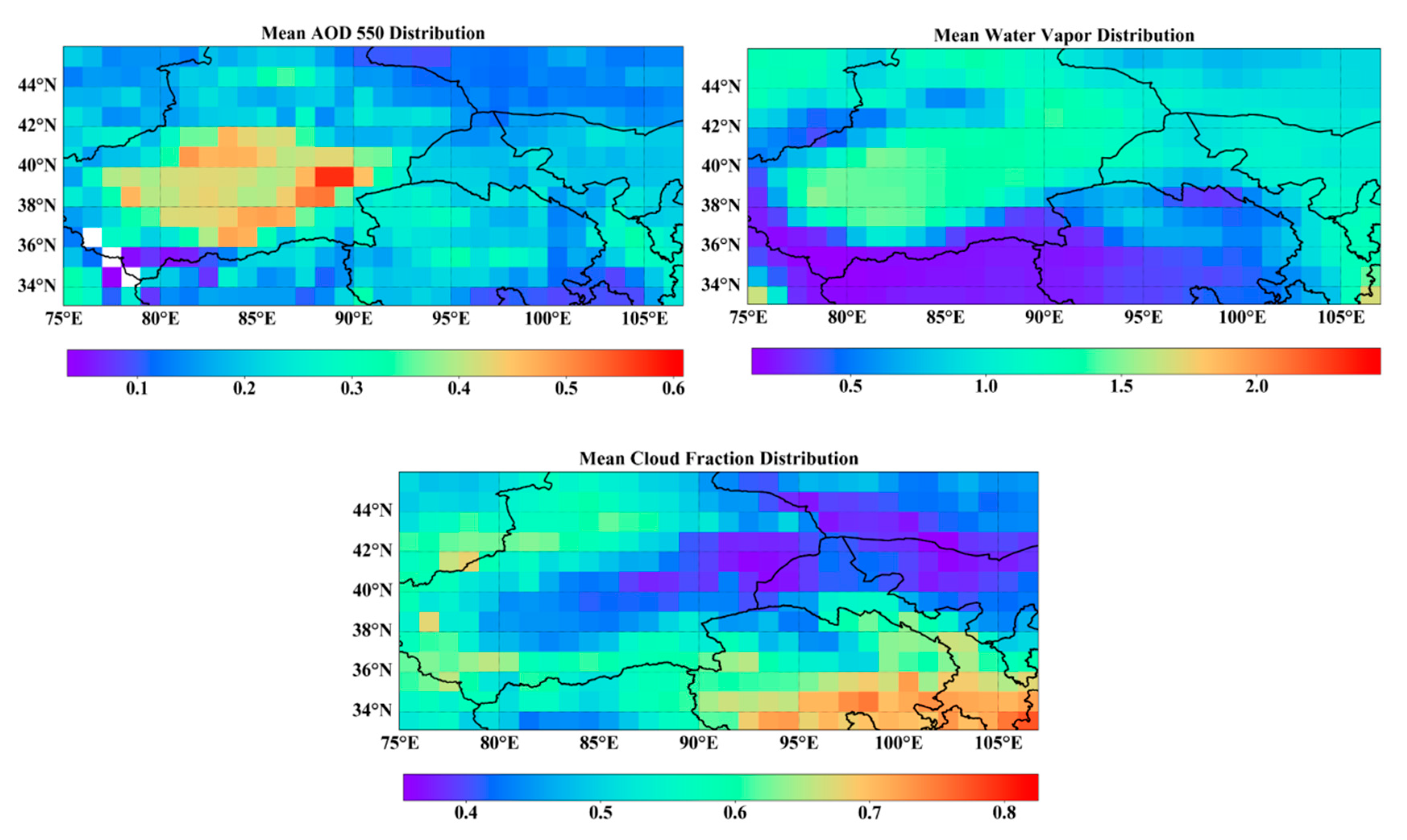
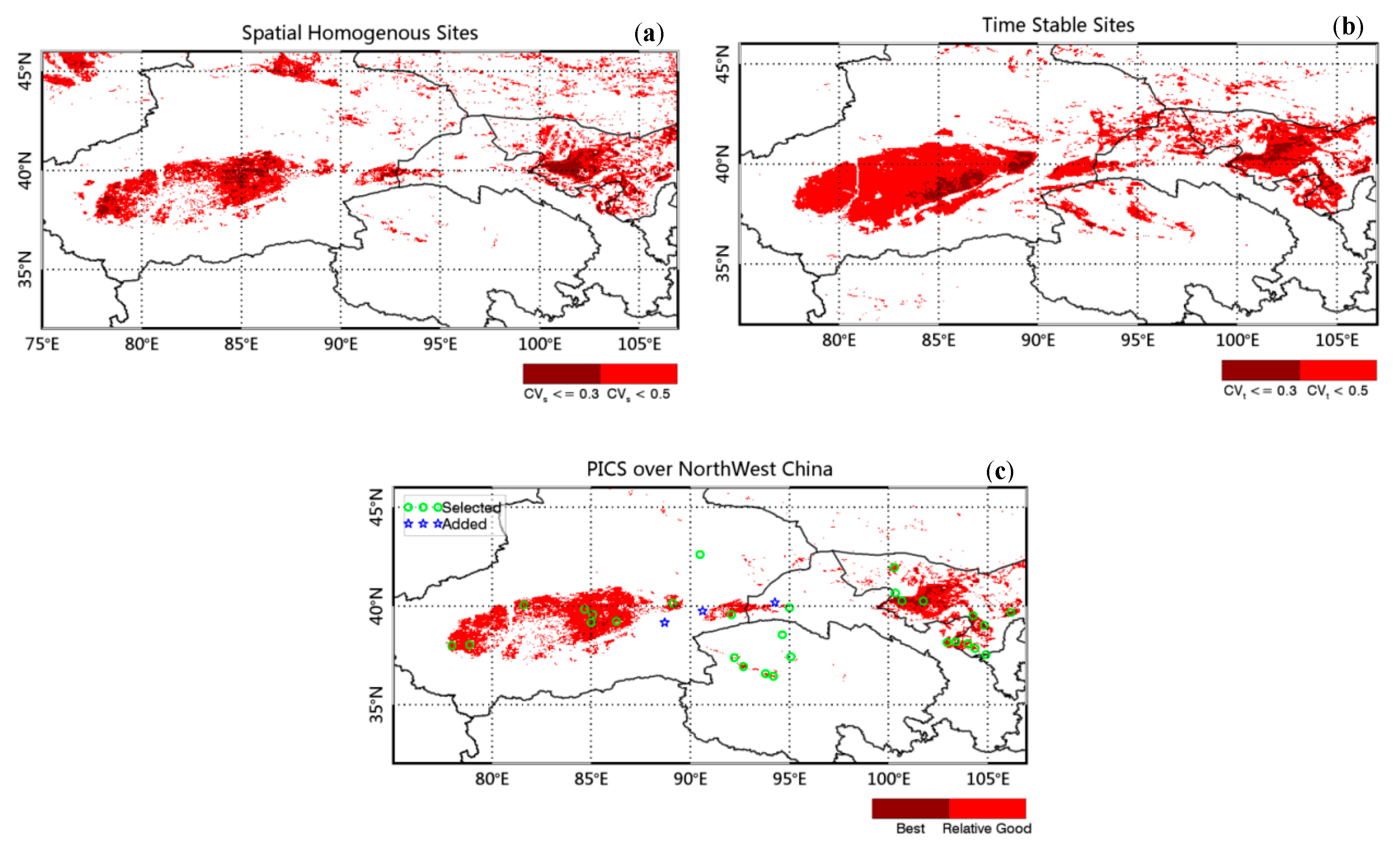
4.1.1. Characterization of the Spatial Uniformity

Figure 3 presents the averaged CV maps of the ROIs derived from the MCD43A3-WSA (V6 collection) images acquired in July of 2002, 2007, 2012, and 2017. The more “homogeneous” areas (CV_s <5% for bands 1,2, 4, and 7) with greater spatial extents were found in the east and the west of the Taklimakan Desert in the Xingjiang Province and the Badain Jaran Desert in the western Inner Mongolia Province. Some “homogeneous” areas with medium-sized spatial extents were observed on the border between eastern Xinjiang and Gansu, where the Kumtag Desert is located, as well as the Tengger Desert, which is to the east of the Badain Jaran Desert. Some “homogeneous” areas with relatively smaller sizes were also found in the Qaidam Basin in Qinghai Province.

4.1.2. Characterization of Temporal Stability

Figure 4 shows the temporal stability of the ROIs derived from MCD43C3-WSA (V5 collection), which were acquired between 01/2008 and 09/2016. Pixels with valid day counts that exceeded 40% of the total day counts in the CV_t calculations are shown in Figure 3. Homogenous areas characterized by CV_t values of less than 4% are shown in blue and green in Figure 3. These areas are desert areas in Northwest China, i.e., three deserts, including the Gilbantungut Desert, Takalamagan Desert, and Kumtag Desert in Xingjiang Province, and four deserts, including the Badain Jaran Desert, Tengger Desert, Ulan Buh Desert, and Kubuqi Desert located in Inner Mongolia Province, and the Qaidam Desert in Qinghai Province. In particular, regions in the Takalamagan Desert, Kumtag Desert, Badain Jaran Desert, and the Tengger Desert had the highest temporal stability over large spatial extents (CV_t of less than 3% on average).

4.1.3. Identification of Optimal Locations Based on CV_s and CV_t

Figure 5a,b illustrate the identified spatially homogeneous and temporally stable areas in the four MODIS bands (bands 1, 2, 4, and 7), using the WSA images acquired from MCD43A3 and MCD43C3 over an approximately 20-y period (2002–2017). The spatially homogenous sites were those that satisfied the criteria of CV_s less than 5% in bands 1, 2, 4, and 7, simultaneously. Similarly, the temporally stable areas had a CV_t of less than 5% for all bands. The spatially homogenous sites and the temporally stable sites presented similar spatial patterns, but the former were spread over relatively smaller areas. The most homogenous and highest temporally stable sites are shown in Figure 5a,b, respectively, in dark red.

Finally, the spatially homogenous sites and the temporally stable sites were overlaid to identify potential PICS, and the results are shown in Figure 5c. The identified CPICS were mainly located in five of the eight deserts in Northwest China. These include the Takalamagan Desert and Kumtag Desert in Xingjiang Province, the Badain Jaran Desert and Tengger Desert, and the Qaidam Desert in Qinghai Province. Note that, due to WSA, which is a fill value in Dunhuang, this site, which is one of the reference PICS endorsed by the CEOS/WGCV/IVOS, is not identified here. The PICS in the Takalamagan Desert and the Badain Jaran Desert present a larger spatial extent than the Kumtag Desert and the Tengger Desert, while the PICS in the Qaidam Desert had several distant pixels. The best PICS sites are shown in dark red in Figure 5c and denote areas that exhibit the lowest spatial variability, as well as temporal variability, i.e., CV_s of less than 3% and a CV_t of less than 3% for the four MODIS bands.

4.2. PICS from IR-MAD

For the previously mentioned IR-MAD-based method, four datasets from the four different sensors were processed to produce four PICS maps. Figure 6 shows an example of an NCP map from a FY3A/VIRR image pair with the interval nearly four years. Figure 7 shows the PICS maps that were identified from the VIRR and MODIS data. Since most pixels in the PICS map had values close to zero, we only selected the top 20% of all pixels for examination and scaled the values to 0–1. As shown in Figure 7, despite the four PICS maps that were produced by the four datasets from different sensors with different timespans, they had consistent results that the high-value pixels (close to 1) were similarly distributed in the study area. This also illustrates that the IR-MAD-based method for PICS identification is not limited to a specific sensor. Subsequently, a suitable threshold can be set as a criterion to define the CPICS of the scene. To get more accurate CPICS, we combined the results from the three VIRR sensors and MODIS by intersecting pixels with values above 0.45 from the four PICS maps. As Figure 8 shows, the CPICS we identified were mainly distributed in the Taklimakan Desert, Kumtag Desert, Badain Jaran Desert, Tengger Desert, and some small Gobi areas.

The IR-MAD-based analysis for PICS identification was generic and fully automatic. The invariant pixels were statistically selected from the image-pair data. This meant that the method was not limited to any specific geographical region or any specific sensor and did not require prior surface knowledge obtained from fieldwork. Additionally, the data used for the IR-MAD analysis was unnecessary to preprocess radiometric normalization due to the invariance property to linear and affine scaling.

The IR-MAD-based analysis of PICS identification was performed as a set of pixel-wise operations and, thereby, did not consider the spatially coherent structures of the image data. In other words, the PICS identified using this novel method were aggregated pixels and were truly temporally stable but not spatially uniform. Two adjacent pixels without similar ground reflectance values could be identified as PICS, on the condition that they were temporally stable during the data acquisition period. Furthermore, for all data not corrected for the BRDF before the IR-MAD analysis procedure, the pixels whose reflectance characteristics were not sensitive to directionality could also be selected as PICS.

4.3. PICS Combined from Using Different Methods

Finally, 29 sites were selected as CPICS according to the CV-based method and the IR-MAD method. Their locations are shown in Figure 5c and Figure 8, as denoted by a green open circle. Another three well-known calibration sites in Dunhuang, Milan, and Luobupohu South were also included here, which are denoted by blue open stars in Figure 5c and as rhombuses in Figure 8. These three sites were not identified using the CV-based method, because the MODIS WSA product had a fill value for the number of days, with an effective pixel count (QF less than 1) of less than 40% in these sites. The central latitude and longitude coordinates of the 32 sites are provided in

Table A1. Name and location of the selected CPICS.

No.	Name	Latitude (°)	Longitude (°)	PICS	Size (km2)	Region	Full Name
1	BDJL_1	40.26	100.679	1	30 × 40	NM	BadainJaran_1
2	BDJL_2	40.25	101.750	1	30 × 40	NM	BadainJaran_2 *
3	BDJL_3	39.512	104.27	1	20 × 25	NM	BadainJaran_3
4	JINT_1	40.653	100.345	1	20 × 25	NM	Jinta_1
5	DXIN_N	41.953	100.288	2	30 × 30	NM	Dingxin_North
6	WUWI_E	38.157	102.951	1	18 × 20	GS	Wuwei_East
7	TNGR_1	38.201	103.395	2	10 × 30	NM	Tengger_1
8	TNGR_2	38.100	103.996	2	15 × 20	NM	Tengger_2
9	TNGR_3	37.857	104.357	2	20 × 8	NM	Tengger_3
10	TNGR_4	39.025	104.831	1	20 × 20	NM	Tengger_4
11	ZHWI_W	37.533	104.904	1	10 × 12	GS	Zhongwei_West
12	LBPO_W	40.145	89.119	2	30 × 30	XJ	Luobupo_West
13	TKLM_1	39.570	85.086	1	30 × 40	XJ	Takalamakan_1
14	TKLM_2	39.231	86.276	2	40 × 50	XJ	Takalamakan_2
15	TKLM_3	40.056	81.618	2	60 × 60	XJ	Takalamakan_3
16	TKLM_4	39.833	84.667	2	40 × 40	XJ	Takalamakan_4 *
17	TKLM_5	39.167	85.00	2	40 × 50	XJ	Takalamakan_5 *
18	DAZH_E	36.450	94.192	1	10 ×10	QH	Dazaohuo_East
19	MANY_S	37.389	92.221	2	11 × 11	QH	Mangya_South
20	DAZH_W	36.581	93.796	2	10 × 8	QH	Dazaohuo_West
21	MOGK_S	39.910	95.000	2	10 × 10	GS	Mogaoku_South
22	SHAN_S	42.604	90.487	2	20 × 20	XJ	Shanshan_South
23	TAERDN	36.939	92.682	2	15 × 15	QH	Taerding
24	XCDH_W	37.432	95.075	2	6 × 6	QH	Xiaochaidan_West
25	SHDBAN	38.721	94.482	2	10 × 10	QH	Shidaoban
26	WULBHE	39.667	106.167	1	20 × 25	NM	Wulanbuhe *
27	KUMTAG	39.566	92.074	1	10 × 15	XJ	Kumtag
28	YECH_E	38.002	77.977	1	30 × 30	XJ	Yecheng_East *
29	PISH_N	38.031	78.871	1	30 × 30	XJ	Pishan_North *
30	DHUNG	40.180	94.270	255	20 × 20	GS	Dunhuang
31	MILAN	39.158	88.709	255	10 × 20	GS	Milan
32	LBPO_S	39.74	90.62	255	18 × 20	XJ	Luobupohu_South

* PICS = “1” means the best site, with both spatial and temporal CVs less than 3%, “2” means a relatively good site, with spatial and temporal CVs less than 5%, and “255” means fill-value, with a fill-value in the spatial or temporal CVs. XJ: Xingjiang Province, NM: Inner Mongolia Province, and GS: Gansu Province. Sites marked with an asterisk in terms of BDJL_2, WULBHE, YECH_E, PISH_N, TKLM_4, and TKLM_5 are collocated or near the sites of China_31, China_36, China_1, China_2, China_15, and China_17, respectively, proposed by Bacour et al. [40].

. As shown in Figure 8 and Table A1, from west to east, the 12 sites are located in Xingjiang Province (abbreviated as XJ in Table A1), six in the Qaidam Desert in Qinghai Province (abbreviated as QH in Table A1), four in Gansu Province (abbreviated as GS in Table A1), and ten in NeiMeng Province (abbreviated as NM in Table A1). Most of the selected sites belong to the category of Gobi deserts, which are composed of sand dunes. Among the 12 CPICS over XJ, nine sites, i.e., TKLM_1 to TKLM_5, YECH_E, PISH_N, LBPO_W, and MILAN are located in the Taklimakan Desert, and the two sites of LBPO_N and KUMTAG are located in the Kumtag Desert. Among the 10 CPICS over NM, three sites in BDJL_1 and BDJL_3 are located in the BadainJaran Deserts, four sites in TNGR_1 and TNGR_4 are located in the Tengger Desert, and one site in WULBHE, the eastern-most site, is located in the Wulanbehe Desert (to the northeast of the Tengger Desert). It should be noted that the BDJL_2, WULBHE, YECH_E, PISH_N, TKLM_4, and TKLM_5 sites were close to the China_31, China_36, China_1, China_2, China_15, and China_17 sites that were, respectively, proposed by Bacour et al. [44]. The sizes of these selected sites were estimated using Google maps, which is also listed in Table A1. Most of the sites have spatial extents of at least 10 km × 10 km, which is suitable for instruments with both large and small footprints, except for TNGR_3, XCDH_W, and DAZH_W. The sites located in the Taklimakan and BadainJaran Deserts, except for BDJL_3, were relatively lager than the other sites and were greater than 30 km × 30 km but more than 60 km × 60 km. These relatively larger sites are comparable in size to the PICS sites of Arabia1, Mauritania1, and Niger1, as proposed by Cosnefroy et al. [8].

These selected CPICS were located at relatively high latitudes in China and much farther north compared to the usual subtropical desert sites, and their reflective surface radiance to outer space are easily affected by incident solar irradiance and surface isotropic features (BRDFs), especially in the winter season when the solar zenith angle is large. However, the relatively low radiances of these sites in winter provide a new opportunity for the vicarious calibrations of the ocean color bands with low radiance dynamics. Furthermore, the increased number of calibration data points allows for the rapid detection of sensor degradation and with increased sensitivity compared to traditional PICS. They also allow for multi-site calibrations (combining several sites together in the calibration curve fitting) of the normal bands with wide dynamics and help us to evaluate and characterize nonlinear instrumental responses by using the wider radiance signals in the summer and winter seasons. However, they cannot be used for vicarious calibrations at some special days when the utilization of these PICSs is limited due to snow in the winter or dust storm events in the spring. The preliminary selected results need more jobs to check if they are good or not by the detailed characterization and utilization tests.

5. Preliminary Characterizations of CPICS and Utilization Demonstration

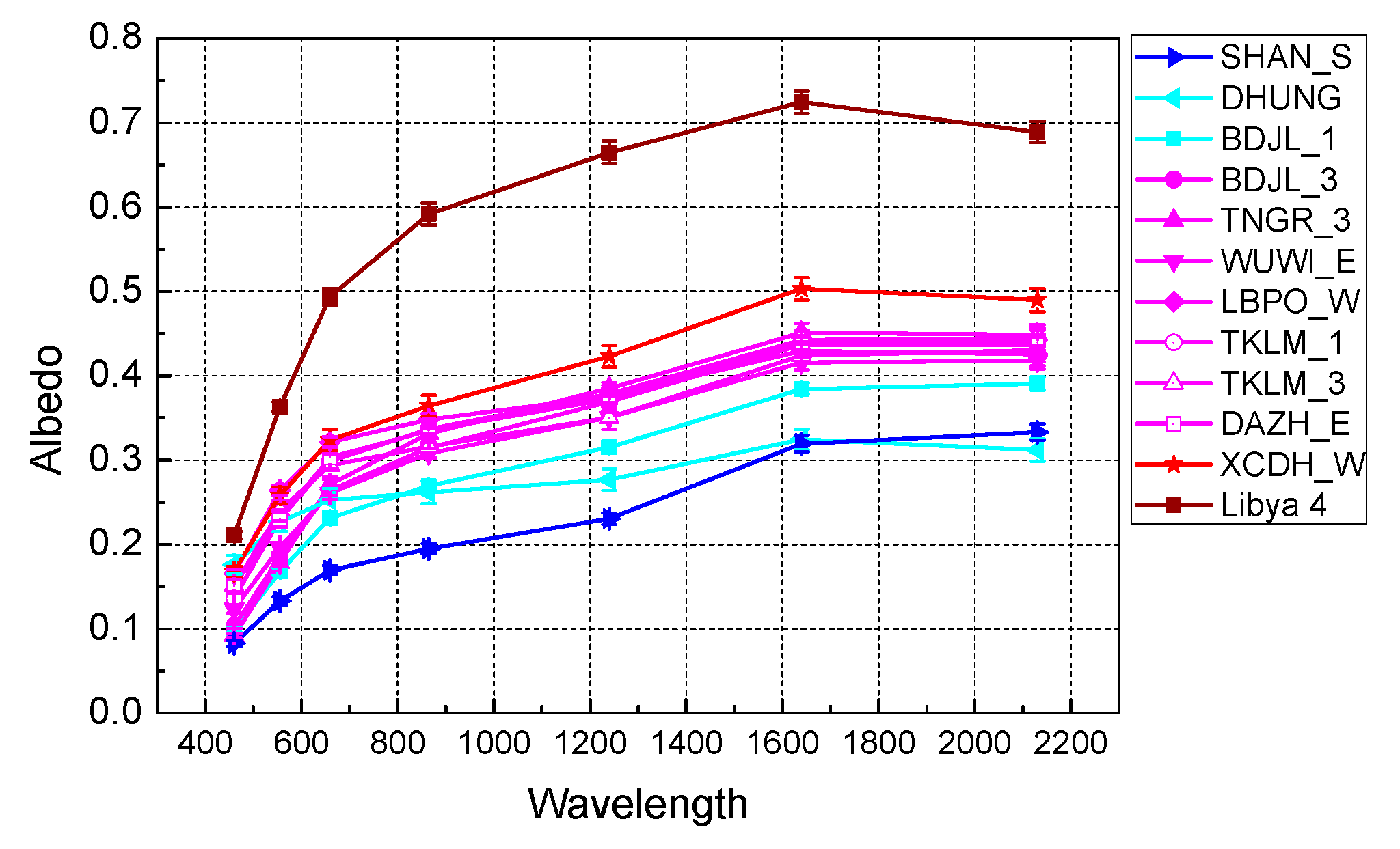
5.1. OLI Images and MODIS Spectral Reflectances of the CPICS

Cloud-free Landsat OLI images were acquired and processed for nine out of the 32 CPICS sites. A sample of these nine images is presented in Figure 9. The images in Figure 9a–d represent areas of 50 km × 50 km centered on the selected sites, and Figure 9e–i represents areas of 20 km × 20 km. Five years of MCD43C1 products from 2013 to 2017 were collected to calculate the surface reflectances of CPICS. Figure 10 shows the averaged spectral reflectances for some CPICS sites, and the averaged spectral reflectance of the most common IVOS site, Libya 4, is also plotted for comparison. The spectral reflectance of each site was calculated using the Ross–Li BRDF model. As shown in Figure 10, the surface reflectances of the CPICS sites are lower than that of Libya 4. By using the wavelength of 865 nm, for instance, Libya 4 has a reflectance level of ~0.6. However, the reflectances of CPICS are between 0.2–0.35. The overall reflectance varies between 0.1 and 0.5 from 460 nm to 2130 nm, which is much flatter than the spectral curve of Libya 4. The relatively high surface reflectance measured over the current PICS, such as Libya 4 in red and near-infrared (typically ~0.5), limits the use of optical sensors at low signal levels (e.g., as typically measured using ocean color sensors over water), due to signal saturation. However, the lower reflectance levels of CPICS may be suitable for assessing the radiometric performances of optical sensors at low signal levels, which further increase the reflectance scope used for stable, oceanic sites, including the so-called “Rayleigh scattering” region for optical sensors at low signal levels.

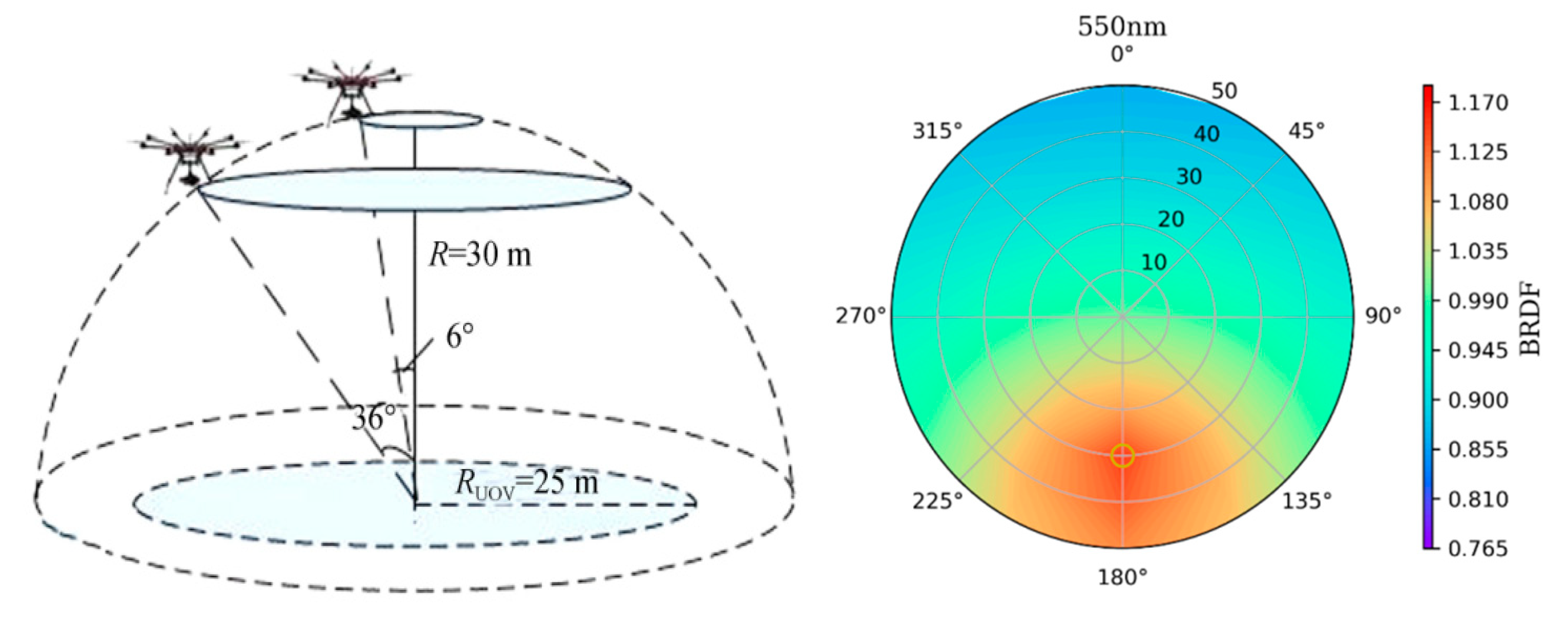
5.2. Characterization of the CPICS Based on Field Campaign Measurements

In August 2019, the National Satellite Meteorological Center led several scientific research institutes, such as the Institute of Optoelectronics of the Chinese Academy of Sciences, to conduct joint field campaigns in Qinghai Province in Northwest China. The characteristics of more than ten sites were measured at the same time, and satellite-ground synchronous radiometric calibrations for domestic multi-series remote-sensing satellites for meteorology, land, and ocean observations were taken into account. The site characteristics mainly included the following three aspects: observation of the directional characteristics of the site using an unmanned aerial vehicle (UAV), observation of surface reflectance spectral using Spectra Vista Corporation (SVC) field spectrometers, and observation of atmospheric parameters such as aerosol by CE318. This paper mainly displayed and analyzed the BRDF and surface spectral characteristics of some selected CPICS over the Qaidam Basin obtained from this field campaign.

The BRDF effect is a key point in remote sensing and oblique photogrammetry. Although surface BRDF is assumed to be radiometrically stable for the Chinese PICSs, it is not expected to be Lambertian. For TOA reflectance levels, a combination of BRDF angular variability and atmospheric temporal/angular variability leads to satellite TOA reflectances that vary from acquisition to acquisition. Coburn et al. presented characterizing sand sites used for PICS through a portable goniometer system, the University of Lethbridge Goniometer System II (ULGS II). The ULGS II is a fully transportable field goniometer system that can be easily moved using all-terrain vehicles [45]. The traditional ground-based BRDF measurement equipment, such as field goniometer systems, are usually a little cumbersome (even if there are some efforts to be portable), making them difficult to be carried and installed in some scenarios. The biggest issue is that the target is easily damaged by the equipment or persons during the measured procedure. With the development of unmanned aerial vehicles (UAV) and other related technologies, there is a new approach to conduct BRDF measurements, with no touching of the target, by the use of UAVs as goniometer platforms.

A UAV-based Goniometer mainly consists of a UAV, a three-axial stabilized pilot platform, and a portable field spectrometer. Using UAV flight line changes and the posture of the pilot platform, the BRDF can be observed and determined from different directions, similar to field a goniometer (Figure 11). The UAV used in this study was a model A660, manufactured by the AZUP Company in Beijing, China and 1700 × 1700 × 500 mm in size. The UAV has an onboard flight controller, and the pilot platform is powered by batteries and has a flight time of 30 min, with an 8-kg load and a maximum load of 10 kg. The spectrometer is an SR-8800 field spectroradiometer, manufactured by Spectral Evolution, MA, USA. It has a full spectral range of 350–2500 nm, with 2151 spectral channels. The minimum spectral resolution is 2.8 nm, and the minimum Field of View (FOV) is 1°. It can be operated through the Internet Tools using the operating system of an iPhone, Android device, or tablet, and it will record the sun height angle, angle of the scan, and GPS location synchronously.

To determine the BRDF characteristics of a given surface, a hemispheric flight pattern for the UAV was developed (Figure 11). The flight pattern acquired a reflectance of 30° steps in the azimuth direction and 10° in the zenith direction, respectively. The position determined the observation angle of the spectrometer, and the pilot platform was stabilized during observation. The radius of the UAV and its surface was 50 m. It took approximately 20 min to fly the entire flight pattern.

The spectrometer works in the DN value mode to measure the ground surface direction reflectance, according to the “standard plate–surface–standard plate” method. It measures the reflected radiance of the reference plate once before and after takeoff and landing and then records the spectral and angle information observed by the spectrometer in sequence during the flight. The standard reference plate used during the test was manufactured by the Remote Sensing Center of the Anhui Institute of Optics and Fine Mechanics, Chinese Academy of Sciences, Anhui, China, and its directional hemisphere reflectance and reflectance factor information were obtained from the laboratory surface. The BRDF of the Xiaochaidan Lake west site are shown in the right panel of Figure 12.

The field spectrometer of SVC HR-1024i with a wavelength range of 350–2500 nm was used to measure the site’s surface reflectance spectrum. The spectral sampling bandwidth, i.e., FWHM (Full Width at Half Maximum) was ≤1.5 nm in the wavelength region of 350–1000 nm, approximately ≤3.6 nm in the wavelength region of 1000–1900 nm, and approximately ≤2.5 nm in the wavelength region of 1900–2500 nm. The field of view was 25°, and the head of the radiometer had a height of 1.5 m. The SVC vertically viewed the same surface every 15 min during the day. Each group consisted of three reference panel observations and three target observations. The intervals between each measurement in one group were short enough to prevent changes in the illumination. The surface reflectance spectrum was the ratio of the average target surface spectrum, and the reference panel spectrum was corrected according to the reference panel BRF that corresponded with the wavelength and the solar zenith angle.

Figure 13a,b depict the reflectance spectra for the Xiaochaidamuhu_west and Shidaoban sites that were measured between 10:00 and 17:00 Beijing Time (BJT). Changes in the sun position during this period caused surface spectral amplitude changes within 10%, but the spectral shape was very stable. By comparing the measured reflectance spectral at 12:00 (BJT) for Xiaochaidamuhu_west and Shidaoban with Dunhuang endorsed by the CEOS Working Group on Cal/Val (WGCV), we found that the brightness of Xiaochaidamuhu_west was higher than Dunhuang above 500 nm, and Shidaoban was lower than Dunhuang below 1500 nm, which was higher than Dunhuang. Compared with Xiaochaidamuhu_west, the reflectance spectra of Dunhuang and Shidaoban were flatter in shape, as shown in Figure 13b. The brightness differences between the three sites contributed to the multi-brightness level calibration field network in China. The Analytical Spectral Devices (ASD) spectral signal is also affected by the atmospheric water absorption around 1400 nm and 1900 nm, so this region is not displayed.

Based on the Terra MODIS atmospheric corrected surface reflectance products MOD09 (V006) and MODIS geolocation MOD03 product with 1-km spatial resolution, we compared the surface reflectance retrieved by Terra MODIS observation and surface reflectance currently measured by SVC. When processing the surface reflectance of MODIS, the BRDF/albedo MCD43C1 model parameters with a spatial resolution of 0.05° were used for BRDF correction, and satellite surface reflectance observations must be corrected before they can be compared with SVC reflectance. As shown in Figure 14, the Terra MODIS satellite observations and the SVC measured surface reflectance were consistent. Overall, the reflectance differences between the SVC observations and the MOD09 were within ±5% regarding MODIS bands 1–7.

Figure 14a,b compares the SVC measured spectral surface reflectance with the near-time Terra MODIS satellite observations of Xiaochaidamuhu_west and Shidaoban, respectively. In this case, SZ is the solar zenith angle, and SA is the solar azimuth. The purpose of precisely characterizing the sites is to further evaluate the possibility of using these sites in the vicarious calibrations. Analysis and verification of the surface spectrum of Xiaochaidamuhu_west and Shidaoban found that the spectral shapes and brightness of both sites met the requirements for a calibration site.

Although the preliminary selection of potential PICS in Northwest China was based on the data from the moderate resolution imagers of Aqua MODIS and FY-3 VIRR, the exact location and profile of each site need to be determined through a more accurate method in the next step, using high spatial resolution. Additionally, more vicarious calibration application cases need taking out to verify the effectiveness of using the selected CPICS to vicariously calibrate different kinds of space-borne sensors in terms of having different spatial and spectral resolutions. The following efforts will focus on vicarious calibration verification using these potential CPICS.

5.3. Demonstration of Vicarious Calibration Using CPICS

The selected Chinese PICS was used to assess the calibration accuracy of the MERSI-II and MODIS instruments, which are found onboard FY3D and Aqua, respectively. This was accomplished through the multi-site calibrations mentioned [46], which compared the satellite measurements with the TOA reflectance simulated by the radiative transfer model (RTM). The key data-processing steps included collecting L1B satellite images over the selected PICS, the selection of a central rectangular ROI, and the exclusion of ROIs due to the presence of clouds. Second, we retrieved the grid-averaged digital counts (DN) and the view-geometry parameters (solar zenith, sensor zenith, and relative azimuth) of the cloud-free ROIs and converted the digital numbers to TOA reflectance using the calibration coefficients provided in the L1B file. Third, we used the 6SV radiative transfer model to obtain the RTM-simulated TOA reflectance over the identified cloud-free ROIs, accounting for the actual solar illumination and sensor viewing angles at the acquisition time, the instrument’s SRFs (Spectral Response Functions), and the corresponding surface and atmospheric properties. Lastly, we performed inter-comparisons of the TOA reflectance between the satellite measurements and the RTM simulations. The details regarding the RTM-simulated TOA reflectance over the PICS can be found in the literature by Wang et al. [46].

Figure 15a–c shows examples of measured MODIS scatterplots and the RTM-simulated reflectance over the selected PICS from data obtained in June, July, November, and December in 2012. Figure 15d–f shows examples of scatterplots from the measured MERSI-II and the RTM-simulated reflectance in June, July, and December 2019 and January 2020. The channels presented here for MODIS consist of bands 1, 2, and 6, with center wavelengths of 650, 865, and 1640 nm. These bands are mostly used for the remote sensing of vegetation. The corresponding MERSI-II channels consist of bands 3, 4, and 6 and are presented in Figure 15d–f, respectively. The averaged satellite (MODIS or MERSI-II) measured TOA reflectance and the relative bias, as well as the root mean square error (RMSE) in the measurements, are also shown in the Figure. It should be noted that, due to an increase in the data range, the RefFactor (the TOA reflectance multiplied by the cosine of the solar zenith angle and divided by the squared Earth–Sun distance) was used instead of the apparent TOA reflectance. There was a high correlation between the simulations and the measurements, all with R values above 0.99 (

Table 2. Radiometric calibration accuracy of Aqua Moderate Resolution Imaging Spectroradiometer (MODIS) and FY-3D Medium Resolution Spectral Imager II (MERSI-II) in the wavelengths of 650, 865, and 1640 nm obtained from vicarious radiometric calibrations using the selected combined pseudo-invariant calibration sites (CPICS) *.

Aqua MODIS					FY-3D MERSI-II
Band	CW (nm)	R	Relative Bias (%)	RMSE (%)	Band	CW (nm)	R	Relative Bias (%)	RMSE (%)
1	650	0.990	3.04	0.04	3	650	0.997	3.87	0.05
2	865	0.988	−1.16	0.03	4	865	0.997	1.34	0.03
6	1640	0.991	1.41	0.04	6	1640	0.996	−5.88	0.88

* CW denotes center wavelength. RMSE: root mean square error.

). The RMSE was less than 0.05% in the listed MODIS channels, indicating that a very small systematic bias exists using the PICS over Northwest China for vicarious calibrations. The validation results of MERSI-II showed that the relative bias and RMSE in the 650 nm and 865 nm of MERSI-II were comparable to that of MODIS, with values of less than ±4% and less than 0.05%, respectively, indicating the sound calibration accuracy and precision of these two channels. The relative bias and the RMSE of 1640 nm for MERSI-II were slightly larger, with values of -5.88% and 0.08%, respectively (Table 2).

The data plotted in Figure 14 are grouped by season. The red scatterplots were obtained in the summer, and the green scatters in the winter. Since the PICS in Northwest China are located in mid-latitude regions, and the incident energy of the sun changes with the seasons, the RefFactor obtained in the summer was larger than in the winter. The “TOA truth” (RTM-simulated TOA reflectance) obtained in the summer was around 0.2–0.4, which was twice that obtained in the winter (0.1–0.2). This increase in the coverage of the sensor dynamic range was helpful for decreasing the calibration uncertainty and allowed for better characterizations for the instrumental nonlinear response problems.

6. Conclusions

This study carried out a full investigation of the overall potential PICSs in Northwest China to meet the requirements of site vicarious calibrations for the increasing number of Chinese remote-sensing satellites. A novel method for selecting PICSs was developed by combined using traditional CV and the newly IR-MAD technique. IR-MAD, which calculates the differences between two multispectral N-band images of the same scene at different times to identify the changing of the image pair, is used to select no-change pixels (NCPs) through one image pair. The IR-MAD method is usually used to find the NCPs of two images at the same place for image normalization or an instrument degradation evaluation. This novel method aggregated plenty of NCPs into PICS sites from a lot of long-term satellite observations at the same place. This method is not sensitive to the calibration accuracy of these satellite observation data, while the traditional temporal CV technique depends on the calibration stability of long-term satellite data. MODIS surface BRDF/albedo products were first used to identify stable sites using spatial and temporal CV analyses, and then, NCPs determined using the IR-MAD method from long-term FY-3/VIRR L1B and MODIS L1B data were aggregated into the stable sites according to their frequency. The results from the CV-based and IR-MAD methods were consistent in most regions in Taklimakan, Badain Jaran, Tengger, Chaidamu, and Kumtag. The combined CPICS results from the two methods were finally verified by the spatial CV of Landsat OLI high-spatial-resolution images and gave the specific location and site size. Their surface features were characterized by MODIS surface products and the field campaign measurements at some sites, including the surface spectral reflectance and BRDF. More than thirty sites were finally determined as potential CPICS from the preliminary selections and characterizations. To demonstrate the practical utilization and usability of these PICSs, they were employed in the multi-site TOA reflectance simulation to validate the operational calibration performance of Aqua/MODIS and FY-3D/MERSI-II. The simulation results showed good consistency compared with the observations from both MODIS and MERSI-II, with a relative bias and RMSE of <5% and <0.05%, respectively. These sites provide prospects for multi-site vicarious calibrations of solar reflective bands, which may help to evaluate or characterize instrumental nonlinear responses using a wider signal dynamic from the sites in different seasons. The significant potential of these selected sites covered the relatively full brightness range of the scene types, which is expected for radiometric calibrations and the temporal stability monitoring of Chinese and international optical satellite sensors.

These CPICS in the northwest were located at relatively high latitudes in China, and their reflective surface radiances to outer space are easily affected by incident solar irradiance and surface isotropic features (BRDFs), especially in the winter season, when the solar zenith angle is larger. Although they have slightly darker surface reflectances, making their SNR (Signal Noise Ratio) lower than that of the subtropical desert sites, they can provide more opportunities for vicarious calibrations for more and more Chinese remote-sensing satellites. Additionally, the relatively low radiance of these sites in the winter provides a good opportunity for the vicarious calibrations of the ocean color bands. They also allow for multi-site calibrations of other normal bands and help to evaluate and characterize nonlinear instrumental responses by using the wider signal dynamic in different seasons. However, they cannot be used for vicarious calibration in some special condition and the utilization of these PICSs is limited due to snow in the winter or dust storm events in the spring. More detailed characterizations of these PICSs in Northwest China and optimal area identifications will be investigated in future works.

References

1. Smith, D.L.; Mutlow, C.T.; Nagaraja Rao, C.R. Calibration monitoring of the visible and near-infrared channels of the Along-Track Scanning Radiometer-2 by use of stable terrestrial sites. Appl. Opt. 2002, 41, 515. [Google Scholar] [CrossRef] [PubMed] [Green Version]
2. Kaufman, Y.J.; Holben, B.N. Calibration of the AVHRR visible and near-IR bands by atmospheric scattering, ocean glint and desert reflection. Int. J. Remote Sens. 1993, 14, 21–52. [Google Scholar] [CrossRef]
3. Teillet, P.M.; Slater, P.N.; Mao, Y. Three methods for the absolute calibration of the NOAA AVHRR sensors in flight. Remote Sens. Environ. 1990, 31, 105–120. [Google Scholar] [CrossRef]
4. Slater, P.N.; Biggar, S.F.; Holm, R.G.; Jackson, R.D.; Mao, Y.; Moran, M.S.; Palmer, J.M.; Yuan, B. Reflectance- and radiance-based methods for the in-flight absolute calibration of multispectral sensors. Remote Sens. Environ. 1987, 22, 11–37. [Google Scholar] [CrossRef]
5. Teillet, P.M.; Barsi, J.A.; Chander, G.; Thome, K.J. Prime candidate Earth targets for the post-launch radiometric calibration of space-based optical imaging instruments. In Earth Observing Systems XII; Butler, J.J., Xiong, J., Eds.; SPIE Proceedings: Sevilla, Spain, 2007. [Google Scholar] [CrossRef]
6. Teillet, P.; Chander, G. Terrestrial reference standard sites for postlaunch sensor calibration. Can. J. Remote Sens. 2010, 36, 437–450. [Google Scholar] [CrossRef]
7. QA4EO. A Quality Assurance Framework for Earth Observation: Principles, 14 January 2010. Available online: http://qa4eo.org/docs/QA4EO_Principles_v4.0.pdf (accessed on 7 December 2019).
8. Cosnefroy, H.; Leroy, M.; Briottet, X. Selection and characterization of Saharan and Arabian desert sites for the calibration of optical satellite sensors. Remote Sens. Environ. 1996, 58, 101–114. [Google Scholar] [CrossRef]
9. Helder, D.L.; Basnet, B.; Morstad, D.L. Optimized identification of worldwide radiometric pseudo-invariant calibration sites. Can. J. Remote Sens. 2010, 36, 527–539. [Google Scholar] [CrossRef]
10. Shrestha, M.; Leigh, L.; Helder, D. Classification of the North Africa Region for Use as an Extended Pseudo Invariant Calibration Sites (EPICS) for Radiometric Calibration and Stability Monitoring of Optical Satellite Sensors. Remote Sens. 2019, 11, 875. [Google Scholar] [CrossRef] [Green Version]
11. Valorge, C.; Meygret, A.; Lebégue, L.; Henry, P.; Bouillon, A.; Gachet, R.; Breton, E.; Léger, D.; Viallefont, F. Forty Years of Experience with SPOT In-flight Calibration. In Post-Launch Calibration of Satellite Sensors–Morain and Budge; Taylor & Francis Group: London, UK, 2004; pp. 119–133. [Google Scholar]
12. Kim, W.; He, T.; Wang, D.; Cao, C.; Liang, S. Assessment of long-term sensor radiometric degradation using time series analysis. IEEE Trans. Geosci. Remote Sens. 2014, 52, 2960–2976. [Google Scholar] [CrossRef]
13. Mishra, N.; Helder, D.; Angal, A.; Choi, J.; Xiong, X. Absolute calibration of optical satellite sensors using Libya 4 pseudo invariant calibration site. Remote Sens. 2014, 6, 1327–1346. [Google Scholar] [CrossRef] [Green Version]
14. Alhammoud, B.; Jackson, J.; Clerc, S.; Arias, M.; Bouzinac, C.; Gascon, F.; Cadau, E.G.; Iannone, R.Q.; Boccia, V. Sentinel-2 Level-1 Radiometry Assessment Using Vicarious Methods from DIMITRI Toolbox and Field Measurements from RadCalNet Database. IEEE J. Sel. Top. Appl. Earth Obs. Remote Sens. 2019, 12, 3470–3479. [Google Scholar] [CrossRef]
15. Govaerts, Y.M.; Clerici, M.; Clerbaux, N. Operational calibration of the Meteosat radiometer VIS band. IEEE Trans. Geosci. Remote Sens. 2004, 42, 1900–1914. [Google Scholar] [CrossRef]
16. Govaerts, Y.M.; Clerici, M. Evaluation of radiative transfer simulation over bright desert calibration sites. IEEE Trans. Geosci. Remote Sens. 2004, 42, 176–187. [Google Scholar] [CrossRef]
17. Bhatt, R.; Doelling, D.R.; Morstad, D.; Scarino, B.R.; Gopalan, A. Desert-based absolute calibration of successive geostationary visible sensors using a daily exoatmospheric radiance model. IEEE Trans. Geosci. Remote Sens. 2013. [Google Scholar] [CrossRef]
18. Chander, G.; Meyer, D.J.; Helder, D.L. Cross calibration of the Landsat-7 ETM+ and EO-1 ALI sensor. IEEE Trans. Geosci. Remote Sens. 2004, 42, 2821–2831. [Google Scholar] [CrossRef]
19. Chander, G.; Angal, A.; Choi, T.; Xiong, X. Radiometric cross-calibration of EO-1 ALI with L7 ETM+ and Terra MODIS sensors using near-simultaneous desert observations. IEEE J. Sel. Top. Appl. Earth Obs. Remote Sens. 2013, 6, 386–399. [Google Scholar] [CrossRef]
20. Pinto, C.; Ponzoni, F.; Castro, R.; Leigh, L.; Mishra, N.; Aaron, D.; Helder, D. First in-flight radiometric calibration of MUX and WFI on-board CBERS-4. Remote. Sens. 2016, 8, 405. [Google Scholar] [CrossRef] [Green Version]
21. Pinto, C.T.; Haque, M.O.; Micijevic, E.; Helder, D.L. Landsats 1-5 Multispectral Scanner System Sensors Radiometric Calibration Update. IEEE Trans. Geosci. Remote Sens. 2019, 1–17. [Google Scholar] [CrossRef]
22. Mishra, N.; Haque, M.O.; Leigh, L.; Aaron, D.; Helder, D.; Markham, B. Radiometric cross calibration of Landsat 8 operational land imager (OLI) and Landsat 7 enhanced thematic mapper plus (ETM+). Remote Sens. 2014, 6, 12619–12638. [Google Scholar] [CrossRef] [Green Version]
23. Bruegge, C.; Coburn, C.; Elmes, A.; Helmlinger, M.C.; Kataoka, F.; Kuester, M.; Kuze, A.; Ochoa, T.; Schaaf, C.; Shiomi, K.; et al. Bi-Directional Reflectance Factor Determination of the Railroad Valley Playa. Remote Sens. 2019, 11, 2601. [Google Scholar] [CrossRef] [Green Version]
24. Angal, A.; Chander, G.; Xiong, X.; Choi, T.; Wu, A. Characterization of the Sonoran desert as a radiometric calibration target for Earth observing sensors. J. Appl. Remote Sens. 2011, 5. [Google Scholar] [CrossRef] [Green Version]
25. Chun, H.-W.; Sohn, B.-J. Climatological Assessment of Desert Targets over East Asia-Australian Region for the Solar Channel Calibration of Geostationary Satellites. Asia-Pac. J. Atmos. Sci. 2014, 50, 239–246. [Google Scholar] [CrossRef]
26. Cook, M. Spatial, Spectral, and Radiometric Characterization of Libyan and Sonoran Desert Calibration Sites in Support of GOES-R Vicarious Calibration; Rochester Institute of Technology, College of Science, Center for Imaging Science: Rochester, NY, USA, 2010. [Google Scholar]
27. Ruchira, T. Worldwide Optimal PICS Searc, Theses, and Dissertations. 1693; South Dakota State University: Brookings, SD, USA, 2017; Available online: http://openprairie.sdstate.edu/etd/1693 (accessed on 7 December 2019).
28. Kizu, S.; Kawamura, H. Degradation of the VISSR visible sensor on GMS-3 during June 1987–December 1988. J. Atmos. Ocean. Technol. 1993, 10, 509–517. [Google Scholar] [CrossRef] [Green Version]
29. Wu, A.; Zhong, Q. A method for determining the sensor degradation rates of NOAA AVHRR channels 1 and 2. J. Clim. Appl. Meteorol. 1994, 33, 118–122. [Google Scholar] [CrossRef] [Green Version]
30. Sohn, B.-J. Selection of Desert Targets, GSICS Webmeeting, for VISIBLE Channel Calibration in the Eastern Hemisphere. 2009. Available online: http://gsics.atmos.umd.edu/pub/Development/20090714/Site-Sel-Web.pdf (accessed on 7 December 2019).
31. GSICS Report in Comparison of Vicarious Calibration Methods and a Strategy to Use Various Land Sites for Inter-Comparison, CGMS-38, NOAA-WP-26. Available online: ftp://ftp.eumetsat.int/pub/CPS/out/CGMS%2038%20report/CGMS-38%20CD/Working%20Papers%20CGMS-38/NOAA/CGMS-38%20NOAA-WP-26.pdf (accessed on 7 December 2019).
32. Hu, X.; Liu, J.; Sun, L.; Rong, Z.; Li, Y.; Zhang, Y.; Zheng, Z.; Wu, R.; Zhang, L.; Gu, X. Characterization of CRCS Dunhuang test site and vicarious calibration utilization for Fengyun (FY) series sensors. Can. J. Remote Sens. 2010, 36, 566–582. [Google Scholar] [CrossRef]
33. Zhang, Y.; Zhong, B.; Liu, Q.; Li, H.; Sun, L. BRDF of Badain Jaran Desert retrieval using Landsat TM/ETM+ and ASTER GDEM data. In Proceedings of the 2011 IEEE International Geoscience and Remote Sensing Symposium, Vancouver, BC, Canada, 24–29 July 2011; pp. 1818–1821. [Google Scholar]
34. Hubanks, P.A.; King, M.D.; Platnick, S.T.; Pincus, R.O. MODIS Atmosphere L3 Gridded Product Algorithm Theoretical Basis Document. Available online: https://eospso.nasa.gov/sites/default/files/atbd/atbd_mod30.pdf (accessed on 19 August 2018).
35. Wolfe, R.E.; Roy, D.P.; Vermote, E. MODIS land data storage, gridding, and compositing methodology: Level 2 grid. IEEE Trans. Geosci. Remote Sens. 1998, 36, 1324–1338. [Google Scholar] [CrossRef] [Green Version]
36. Bannari, A.; Omari, K.; Teillet, P.M.; Fedosejevs, G. Potential of Getis statistics to characterize the radiometric uniformity and stability of test sites used for the calibration of Earth observation sensors. IEEE Trans. Geosci. Remote Sens. 2005, 43, 2918–2926. [Google Scholar] [CrossRef]
37. Odongo, V.; Hamm, N.A.S.; Milton, E.J. Spatio-Temporal Assessment of Tuz Gölü, Turkey as a Potential Vicarious Calibration Site. Remote Sens. 2014, 6, 2494–2513. [Google Scholar] [CrossRef] [Green Version]
38. Gu, X.F.; Guyot, G.; Verbrugghe, M. Evaluation of measurement errors in ground surface reflectance for satellite calibration. Int. J. Remote Sens. 1992, 13, 2531–2546. [Google Scholar] [CrossRef]
39. Gürbüz, S.Z.; Özen, H.; Chander, G. A Survey of Landnet Sites Focusing on Tuz Gölü Salt Lake, Turkey. In Proceedings of the International Archives of the Photogrammetry, Remote Sensing and Spatial Information Sciences, Melbourne, Australia, 25 August–1 September 2012; pp. 115–120. [Google Scholar]
40. Chander, G.; Xiong, X.X.; Choi, T.Y.; Angal, A. Monitoring on-orbit calibration stability of the Terra MODIS and Landsat 7 ETM+ sensors using pseudo-invariant test sites. Remote Sens. Environ. 2010, 114, 925–939. [Google Scholar] [CrossRef]
41. Nielsen, A.A.; Conradsen, K.; Simpson, J.J. Multivariate alteration detection (MAD) and MAF postprocessing in multispectral, bitemporal image data: New approaches to change detection studies. Remote Sens. Environ. 1998, 64, 1–19. [Google Scholar] [CrossRef] [Green Version]
42. Nielsen, A.A. The regularized iteratively reweighted MAD method for change detection in multi-and hyperspectral data. IEEE Trans. Image Process. 2007, 16, 463–478. [Google Scholar] [CrossRef] [PubMed] [Green Version]
43. Canty, M.J.; Nielsen, A.A. Automatic radiometric normalization of multitemporal satellite imagery with the iteratively re-weighted MAD transformation. Remote Sens. Environ. 2008, 112, 1025–1036. [Google Scholar] [CrossRef] [Green Version]
44. Bacour, C.; Briottet, X.; Bréon, F.-M.; Viallefont-Robinet, F.; Bouvet, M. Revisiting Pseudo Invariant Calibration Sites (PICS) Over Sand Deserts for Vicarious Calibration of Optical Imagers at 20 km and 100 km Scales. Remote Sens. 2019, 11, 1166. [Google Scholar] [CrossRef] [Green Version]
45. Butler, J.J.; Xiong, X.X.; Coburn, C.A.; Gu, X.; Logie, G.; Beaver, J. Temporal dynamics of sand dune bidirectional reflectance characteristics for absolute radiometric calibration of optical remote sensing data. In Proceedings of the SPIE Optical Engineering, San Diego, CA, USA, 24–28 August 2016; p. 99720J. [Google Scholar] [CrossRef]
46. Wang, L.; Hu, X.; Chen, L.; He, L. Consistent Calibration of VIRR Reflective Solar Channels Onboard FY-3A, FY-3B, and FY-3C Using a Multisite Calibration Method. Remote Sens. 2018, 10, 1336. [Google Scholar] [CrossRef] [Green Version]
Figure 1. RGB (Red, Green and Blue) clear sky composite map of the study area from FY-3D/Medium Resolution Spectral Imager II (MERSI-II) in October.
Remotesensing 12 02517 g001
Figure 2. Spatial distributions of the main atmospheric variables between 2008–2018 in Northwest China. AOD: aerosol optical depth.
Remotesensing 12 02517 g002
Figure 3. Spatial coefficient of variation (CVs) maps for the regions of interest (ROIs) in Moderate Resolution Imaging Spectroradiometer (MODIS) bands 1, 2, 4, and 7, calculated from MCD43A3 in July of 2002, 2007, 2012, and 2017. The black pixels are those excluded in the CVs calculations according the quality flag (QF) values provided in the MCD43A3 products.
Remotesensing 12 02517 g003
Figure 4. Temporal coefficient of variation (CVt) maps for the regions of interest (ROIs) in MODIS bands 1, 2, 4, and 7 calculated from MCD43C3 between 01/2008–09/2016. The black pixels are those excluded in the CVt calculations according the QF values provided in the MCD43C3 products.
Remotesensing 12 02517 g004
Figure 5. (a) Spatial homogenous sites, (b) temporal stable sites, and (c) final selected pseudo-invariant calibration sites (PICS) over Northwest China.
Remotesensing 12 02517 g005
Figure 6. An example of a FY3A/visible infrared radiometer (VIRR) image pair with the interval of nearly four years. The upper two pictures are the true-color images of the two scenes (a,b), respectively; the lower picture (c) is the no-change pixel (NCP) map obtained from the image pair through the iteratively reweighted multivariate alteration detection (IR-MAD) procedure.
Remotesensing 12 02517 g006
Figure 7. NCP aggregation (relative frequency) maps of the IR-MAD-based method for PICS identification from the four sensor datasets.
Remotesensing 12 02517 g007
Figure 8. Combined pseudo-invariant calibration sites (CPICS) map of the results from three VIRRs and MODIS.
Remotesensing 12 02517 g008
Figure 9. Landsat operational land imager (OLI) RGB composite maps of several typical combined pseudo-invariant calibration sites (CPICS). The image size of the first four sites is 50 × 50 km2 (ad), which means larger sites, and 20 × 20 km2 for the other five sites, which are relatively smaller sites (ei).
Remotesensing 12 02517 g009
Figure 10. Averaged spectral reflectance curves for some common combined pseudo-invariant calibration sites (CPICS) sites, including Libya 4, acquired from MODIS bidirectional reflectance distribution function (BRDF) products between 2013–2017. For CPICS, to avoid dust events and snowy weather, the months from May to October were included in the calculation. For Libya 4, all the months are included. The error bars in the curves denote the standard deviations of the reflectance spectra.
Remotesensing 12 02517 g010
Figure 11. Unmanned aerial vehicle (UAV)-based goniometer.
Remotesensing 12 02517 g011
Figure 12. Hemispheric flight pattern for the unmanned aerial vehicle (UAV) (Left) and bidirectional reflectance distribution function (BRDF) of the Xiaochaidan Lake west site (08/13/2019) (Right).
Remotesensing 12 02517 g012
Figure 13. (a) Mean surface reflectance spectra of Xiaochaidamhu_west and Shidaoban when the solar zenith less than 30°, and the shaded area is the standard deviation; (b) comparison of the surface reflectance spectra of Xiaochaidamuhu_west, Shidaoban, Dunhuang, Dazaohuo_w, and Dazaohuo_E measured at a specific time.
Remotesensing 12 02517 g013
Figure 14. SVC (Spectra Vista Corporation) measured surface reflectance spectra obtained within 1 h before and after the Terra MODIS pastime. (a) Xiaochaidamuhu_west and (b) Shidaoban. SZ is the solar zenith angle, and SA is the solar azimuth. The shaded area is the standard deviation of the SVC observations.
Remotesensing 12 02517 g014
Figure 15. Scatterplots of the satellite measurements and simulated reflectance over the pseudo-invariant calibration sites (PICS) in Northwest China: (ac) for Aqua MODIS in June, July, November, and December 2019; (df) FY3D MERSI-II in June, July, and December 2019 and January 2020. The 1:1 line is shown as a dashed line, and the calibration relative bias and root mean square error (RMSE) in the MERSI-II top of atmosphere (TOA) reflectance against the radiative transfer model (RTM) simulations are labeled.
Remotesensing 12 02517 g015