Article

Landslide Susceptibility Assessment of Wildfire Burnt Areas through Earth-Observation Techniques and a Machine Learning-Based Approach

by
Mariano Di Napoli
1,
Palmira Marsiglia
2,
Diego Di Martire
2,*,
Massimo Ramondini
3,
Silvia Liberata Ullo
4 and
Domenico Calcaterra
2
1
Department of Earth, Environment and Life Sciences, University of Genoa, Corso Europa, 26, 16132 Genoa, Italy
2
Department of Earth, Environment and Resources Sciences, Federico II University of Naples, Complesso Universitario di Monte Sant’Angelo, Via Cinthia, 21, 80126 Naples, Italy
3
Department of Civil, Architectural and Environmental Engineering, Federico II University of Naples, Via Claudio, 21, 80125 Naples, Italy
4
Engineering Department, University of Sannio, Piazza Roma, 21, 82100 Benevento, Italy
*
Author to whom correspondence should be addressed.
Remote Sens. 2020, 12(15), 2505; https://doi.org/10.3390/rs12152505
Submission received: 2 July 2020 / Revised: 23 July 2020 / Accepted: 30 July 2020 / Published: 4 August 2020
(This article belongs to the Section Remote Sensing in Geology, Geomorphology and Hydrology)

Abstract

:
Climate change has increased the likelihood of the occurrence of disasters like wildfires, floods, storms, and landslides worldwide in the last years. Weather conditions change continuously and rapidly, and wildfires are occurring repeatedly and diffusing with higher intensity. The burnt catchments are known, in many parts of the world, as one of the main sensitive areas to debris flows characterized by different trigger mechanisms (runoff-initiated and debris slide-initiated debris flow). The large number of studies produced in recent decades has shown how the response of a watershed to precipitation can be extremely variable, depending on several on-site conditions, as well as the characteristics of precipitation duration and intensity. Moreover, the availability of satellite data has significantly improved the ability to identify the areas affected by wildfires, and, even more importantly, to carry out post-fire assessment of burnt areas. Many difficulties have to be faced in attempting to assess landslide risk in burnt areas, which present a higher likelihood of occurrence; in densely populated neighbourhoods, human activities can be the cause of the origin of the fires. The latter is, in fact, one of the main operations used by man to remove vegetation along slopes in an attempt to claim new land for pastures or construction purposes. Regarding the study area, the Camaldoli and Agnano hill (Naples, Italy) fires seem to act as a predisposing factor, while the triggering factor is usually represented by precipitation. Eleven predisposing factors were chosen and estimated according to previous knowledge of the territory and a database consisting of 400 landslides was adopted. The present work aimed to expand the knowledge of the relationship existing between the triggering of landslides and burnt areas through the following phases: (1) Processing of the thematic maps of the burnt areas through band compositions of satellite images; and (2) landslide susceptibility assessment through the application of a new statistical approach (machine learning techniques). The analysis has the scope to support decision makers and local agencies in urban planning and safety monitoring of the environment.

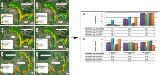
Graphical Abstract

1. Introduction

Landslides are responsible worldwide for significant socioeconomic losses and, historically, have taken on a fundamental position in the list of natural hazards affecting the Italian territory [1,2,3,4]. In urban areas, the impact of these phenomena is further exacerbated by the high population density and a large number of buildings and infrastructures [5,6,7,8,9,10]. After the Second World War, urban centres experienced a huge demographic and, consequently, physical expansion. In the case of the city of Naples, this massive urban expansion has often developed under the banner of illegalism, so that the concept of an “illegal city” has been introduced [11]. In fact, over a few decades, huge neighbourhoods have grown rapidly, reaching a rather high population density of 6000–7000 inhabitants per square kilometer. In many cases, these areas are exposed to natural hazards, such as floods and landslides [8,12]. Recent and repeated landslides, in Naples and other sites in Campania, have created awareness of the landslide hazard in the region, and have encouraged engineering geologists and local administrators to undertake research activities aimed at risk assessment and mitigation. The city of Naples has been declared a national priority in terms of the mitigation of landslide risk by the Italian government [13]. Currently, Naples is a city with high territorial “fragility”, as it is characterized by a complex and often chaotic urban fabric that exists in an extremely complex geological and geomorphological context [14]. It is made even more fragile by a multitude of underground artificial cavities as a result of past mining activities. Since large portions of the metropolitan area of Naples are located in hilly areas, the instability of the slopes must be taken into consideration. The Camaldoli and Agnano hills are emblematic since these hills experience fire almost every year. As a result, both areal and linear erosion phenomena have occurred in the burnt sectors of the slope (Figure 1).
One of the most dangerous post-wildfire effects is the generation of debris flows [15,16,17]. Debris flows are able to carry large quantities of materials over relatively gentle slopes and may generate an elevated impact force that provokes remarkable destruction of buildings [18]. The burnt catchment areas are known, in many parts of the world, as being among the sites most sensitive to debris flows [15,19] characterized by different trigger mechanisms (runoff-initiated and debris slide-initiated debris flows). Wildfires can produce radical variations in the runoff response of a burnt watershed. Removal of the rainfall-intercepting vegetation, soil mantling organic matter that protects the soil from raindrop impact and slow runoff, the presence of wood ash on burnt soils, and the generation of water-repellent soils can result in significant changes in the infiltration and runoff properties compared to pre-fire conditions [20,21]. Indeed, infiltration generally decreases because the chemical [22,23] and physical [23,24,25] properties of the soil may have changed, making the soil more water repellent. Given the spatial heterogeneity of the soil characteristics following the occurrence of wildfires, even low-intensity and short-duration rainfalls can generate instability phenomena [20]. Many studies produced in recent decades have shown how the catchment response to rainfall can be extremely variable, depending on several on-site conditions, as well as the characteristics of the duration and intensity of rainfall [17,18,20,21,26]. Many difficulties need to be addressed in an attempt to assess landslide risk in burnt areas; they are even higher in densely populated neighborhoods, where the presence of man and his activities can be at the origin of fires (they are, in fact, one of the main operations used by man to remove vegetation along the slopes in an attempt to claim new land for pasture or construction purposes). As evidenced in the scientific literature, wildfires seem to act as a predisposing factor, which is then triggered by rainfall [27,28,29]. The latter consideration has been confirmed in a similar geological context concerning the Campania region (Sarno Mountains) by [30] and for the study area by [31]. In recent years, the use of satellite data has significantly improved the ability to monitor the Earth surface and analyze the presence of vegetated areas, which can alert on the possibility of future fire risks, with as-specified consequences [32,33]. Even more interesting, satellite data can be processed to build digital elevation models (DEMs) and use them to measure landslide effects in terms of soil movement, as shown in [34]. Referring to the importance of identifying the areas affected by wildfires, a detailed analysis was carried out on the post-fire assessment of burnt areas in [35,36], where data from satellites with a low revisit time were combined to low-spatial-resolution satellite data.
Landslides susceptibility assessment (LSA) has been conducted using machine learning algorithms (MLAs), with or without satellite data combination [37]. In the latter, MLAs have been demonstrated to be a better strategy for natural hazard estimates, with four different types of algorithms ensembled to assess landslide susceptibility, which include the artificial neural network (ANN), generalized boosting (GBM), random forests (RFs), and maximum entropy (MaxEnt), being employed. Eleven predisposing factors (PFs) have been considered, based on the knowledge of the territory and of shallow rapid landslide mechanisms: Slope angle, aspect angle, geo-lithology, planform curvature, profile curvature, streams density, distance to streams, land use, topographic wetness index (TWI), topographic position index (TPI), and wildfires. The final result is, therefore, a susceptibility map computed by an average of the values of the occurrence probability previously obtained.
Given all the above considerations, in the present manuscript, the authors aimed to expand knowledge of the landslides on the Camaldoli and Agnano hillslopes. This work was conducted through a combined study of machine learning techniques, for the LSA, and employing satellite techniques and data processing for the survey of burnt areas that occurred annually in the study area. The results were then validated through field investigations.

2. Geological and Geomorphological Setting

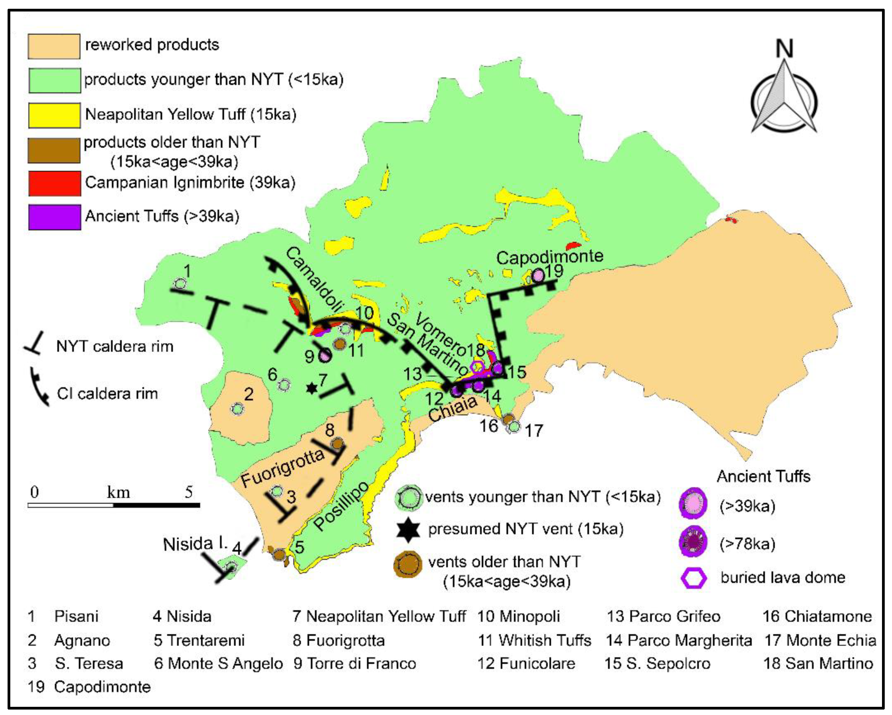
Phlegraean Fields are a volcanic field characterized by a resurgent caldera generated by the superposition of two volcano-tectonic collapses linked to the eruptions of the Campanian Ignimbrite (CI—39 ka [38]) and Neapolitan Yellow Tuff (NYT—15 ka [39]) [40,41]; the city of Naples lies on the easternmost part of the Phlegrean Fields. The volcanic history of the Phlegraean Fields has been characterized by a large number of mainly explosive eruptions, which have given rise to mainly monogenic buildings and have put in place huge volumes of pyroclastic and, to a lesser extent, effusive rocks. Phlegraean volcanism includes not only the activity developed on the continent but also that developed on the islands of Ischia and Procida [42]. Although the beginning of volcanism in the area is not precisely defined, the oldest dated rocks, which are not the lowest ones in the stratigraphic sequence, indicate an age of about 60 ka [43] and are related to the explosive volcanism, which extended beyond the current margin of the Phlegraean caldera.
The first event that strongly influenced the geological and structural evolution of the area was the eruption of the Campanian Ignimbrite (CI). This eruption extruded at least 200 km3 of magma [44] and was accompanied by the collapse of a large caldera of about 230 km2, which included the city of Naples, the Phlegraean Fields, and part of the bays of Naples and Pozzuoli. Pyroclastic rocks, mainly consisting of diluted and turbulent pyroclastic currents, over an area of about 30,000 km2, have significantly changed the landscape. After the Campanian Ignimbrite, between 39 and 15 ka, volcanism concentrated within the collapsed area, with mainly explosive and subordinately effusive eruptions that generated pyroclastic deposits, tuff cones, and lava domes. The second most significant event in the history of the Phlegraean Fields was the freato-magmatic eruption of the Neapolitan Yellow Tuff (NYT), which brought at least 40 km3 of magma per day and generated a wide caldera of about 90 km2 inside the previous caldera of the Campanian Ignimbrite. Pyroclastic currents and fall deposits have been placed on an area of over 1000 km2, especially north-east of the source. The deposits of the two largest eruptions in the Phlegraen area have been used as stratigraphic markers, thanks to which volcanic activity, and therefore geological history, is conventionally divided into three periods [45] (Figure 2). Specifically, as regards the city of Naples, the NYT constitutes the backbone of most of the Neapolitan hills. The volcano-tectonic processes of the last 39 ka have significantly contributed to the current structure of the Neapolitan and Phlegrean areas. In some cases, the original volcanic morphologies have been modelled or partially dismantled by tectonic and volcano-tectonic events and by the intense erosion-deposition processes of pyroclastic products [13]. Some depressions within the NYT caldera have been periodically submerged by the sea, as demonstrated by the type of sediments and the presence of depositional morphologies or erosion (marine terraces, cliffs). The general subsidence of Phlegraean Fields and the resurgence of the central portion of the NYT caldera also contributed to the complex morphology of the area.

3. Definition and Characteristics of Wildfires

As stated in Italian Law 353/2000 (framework Law on Wildfires), a wildfire is defined as a fire with susceptibility to expand on wooded, bushy, or arboreal areas, including any anthropized structures and infrastructures placed within the aforementioned areas, or on cultivated or uncultivated land and pastures adjacent to these areas. In a forest, there is a large amount of fuel (vegetation) and comburent (air), but a fire can only occur in the presence of the ignition. Three fire propagation regimes can be distinguished [46]:
  • Ground fire, which burns without a flame in the organic layer above the mineral soil; its propagation is very slow and it can produce considerable damage to the soil, given its long residence time;
  • Surface fire, which represents the most common fire propagation regime, during which a large class of plant substrate close to the topographic surface is consumed in flame combustion;
  • Crown fire, which occurs when a surface fire that spreads under arboreal vegetation extends to the upper layers of the foliage; this fire can burn a single tree or a group of trees.
The hydrological and geomorphological consequences of a violent fire depend on its frequency and intensity. The frequency varies widely depending on the type of vegetation and the climate [47]. Climate change and the recent action of man have increased the return time of the fires, causing an alteration of the quantity and characteristics of the “fuel”. The severity of a fire is commonly, though not always, classified according to the degree of destruction of life above the ground and the death of biomass (which is a function of the type of fuel), and is based on the quantity, the characteristics, the intensity, and the duration of the fire [48]. Despite the clear importance for understanding hydrological and morphological impacts following fire [19,49,50], the existing severity classifications are not useful, predictive, or reliable tools to interpret critical soil changes following fire [46]. The heat produced during fires has significant effects on soil, inducing both physical and chemical changes [22,25,51]. Processes that are triggered in the soil layer develop progressively
With increasing temperature and have been thoroughly studied by [23,25,52,53]. Starting from temperatures of 40–70 °C begins the disintegration of living tissues, and all microbes begin to be affected between 50 and 120 °C. At higher temperatures (>220 °C) physical-chemical changes occur with the aggregation of silt and clay to originate sandy cutting particles, and between 200 and 315 °C, there is the distillation of the organic content, and the volatilization of nutrients at 200–400 °C [48]. It is under such conditions that water repellency develops and/or increases, which involves a decrease in permeability and an increase in surface runoff; for this reason, in conjunction with meteorological events, even if not extreme, mass transport phenomena can be generated, even large ones [54]. Formation of the water-repellent layer is attributed to the polymerization of the organic molecules into more hydrophobic compounds that adhere more to the soil particles, also forming the binder and the filling of the pores to originate macro-aggregates with soil grains [25,55,56]. The temperatures necessary for the explanation of these processes are easily reached on the surface, but it is only under particularly severe fire conditions that temperatures of 200–300 °C penetrate beyond the 2-cm depth [57]. The persistence over time of the hydrophobic horizon is very limited; in fact, after the wet season, traces on the soil of the water-repellent layer are minimal [58].
Summing up, on a pedological level, the main consequences of the passage of fire are therefore the tendency for soil reduction, erosion of the superficial soil layers, and an increase of the surface runoff [46,59]; these effects occur mainly during the first year after the passage of the fire. The persistence over time of the effects induced by fire on the soil depends on several factors. In particular, these changes can exist for a few minutes or even for a few years: According to many authors, a period of 1–2 years must be considered as the minimum time interval for the soil recovery process to be visible [5,18,18,21,60,61,62,63,64,65].
Wildfires can be triggered by both natural and anthropogenic causes. However the percentage of fires whose origin is attributable to natural causes is very low: In Italy, according to data from the State Forestry Corps, only about 1% of the total belongs to this category of events. It can, therefore, be easily deduced that human action is the main cause of the fire. The problem of forest fires is therefore particularly evident in Italy and, in fact, in our country, although lagging behind other parts of the world (e.g., the USA) and continent (e.g., France), there are two legislative measures, namely the Forestry Law 3267/1923 and Law 353/2000.

4. Materials and Methods

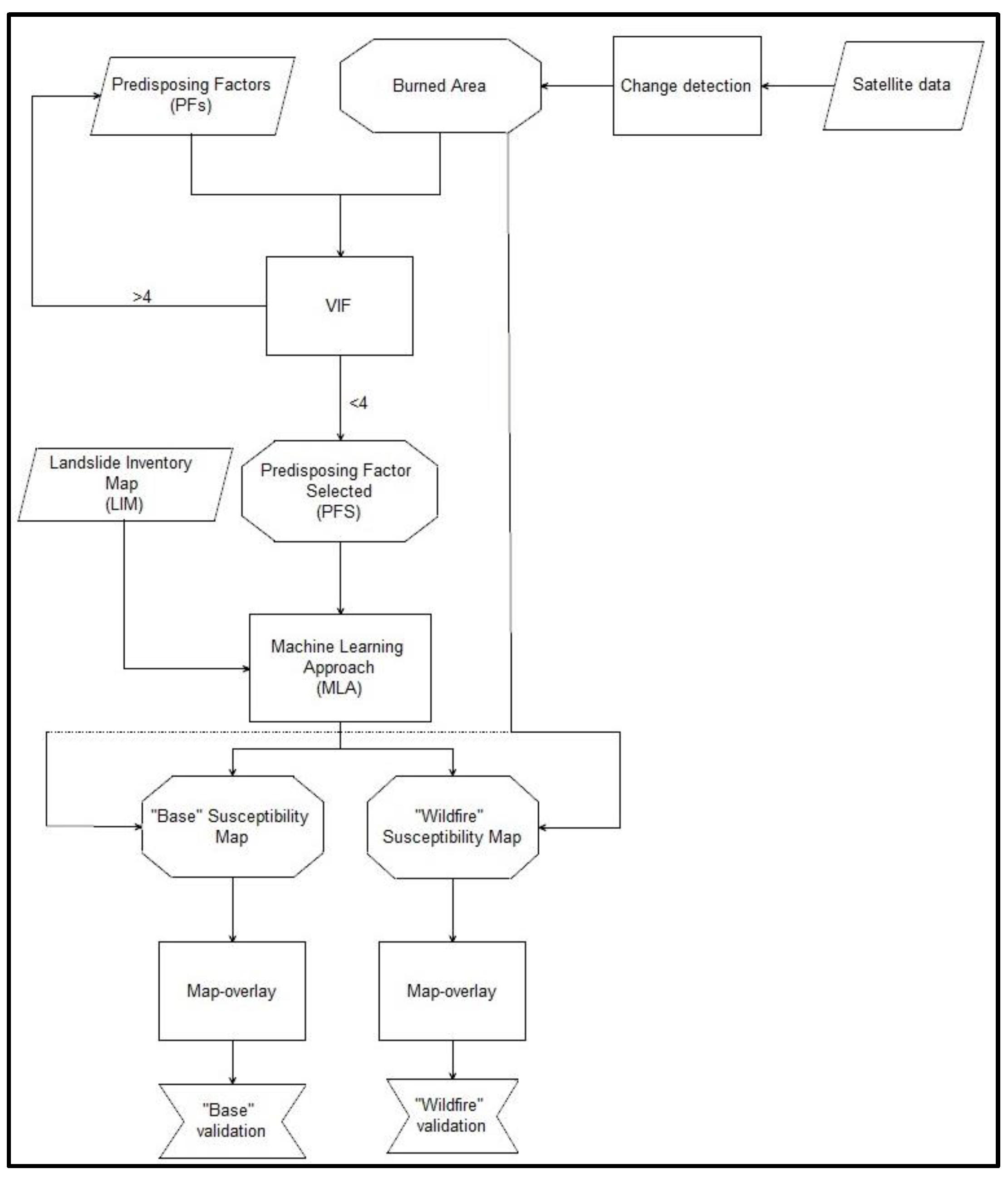
Figure 3 shows a flow chart of the implemented approach, which was composed of different steps: (1) Change detection analysis for burned area assessment and PFs preparation, (2) multicollinearity test using VIF, (3) modelling of landslide and preparation of landslide susceptibility map, and (4) map overlay with validation of the results.

4.1. Landslide Inventory

The landslide inventory map (LIM) is the basis for any landslide susceptibility assessment. An accurate and reliable landslide inventory data is crucial for landslide susceptibility modelling [66,67]. In this study, an extensive database (more than 1300 landslides), covering the 1816–2015 time-span, was initially used [8,68]. The LIM was then updated until February 2020, analyzing the Google Earth satellite images and through field investigation. A total of 384 events, 230 for the Camaldoli hill and 154 for the Agnano hills, were recognized and classified according to previous studies [69,70]. The LIM used in this work was obtained taking into account only those landslides characterized by rapid kinematics and involving shallower levels of the loose pyroclastic deposits. All the landslides selected can be classified as a debris slide and many landslides with a complex evolution can be observed along the slopes. Due to the reduced areal distribution (ranges from 10 to 100 m2), landslides were used as point features, and were positioned in the upper part of the triggering zone.

4.2. Landslide Predisposing Factors

Based on the knowledge and characteristics of the area, 11 predisposing factors were identified as a basis for the landslide susceptibility assessment: Slope angle, slope aspect, profile curvature, planform curvature, distance to streams, streams density, geo-lithological map, topographic wetness index (TWI), topographic position index (TPI), land use, and wildfire. The predisposing factors were prepared using a digital terrain model (DTM) with 5 × 5 m resolution cells, obtained from a regional technical map (scale 1:5000).

4.2.1. Slope Angle

Slope angle is notoriously one of the most significative predisposing factors in landslide occurrence and it is defined as the angle between the horizontal and the slope’s topographic surface. Gravity is an inner strength with external results, which are present everywhere. The slope determines how much of that force is efficacious in inducing the object to move; the steeper the hill, the bigger the slope angle, and the greater the component of the gravitational force, which produces the movement. Regarding the study area, the loose pyroclastic soils are mainly affected in slides on open slopes and in debris flows on channelled slopes [8]. Such slope failures are shallow, originate on sides steeper than 35°, and demonstrate a limited runout potential [1]. So, the steepness of the slope can be proposed as the most essential terrain-related risk factor concerning slope stability [71].

4.2.2. Slope Aspect

Slope aspect plays a fundamental role in controlling soil moisture along slopes through solar radiation and rainfall [72]. The value of each cell in an aspect dataset indicates the direction of the cell’s slope facing. Besides, the slope aspect can indirectly affect landslide processes because it controls the duration of sunlight, evapotranspiration, moisture retention, vegetation cover type, and vegetation distribution [73]. Slope aspect values range between 0 and 360 degrees.

4.2.3. Planform and Profile Curvature

Slope shape has long been used as the basis of geomorphological evaluations for studies dealing with landslides, groundwater, and karst. Slopes not only include a large part of the natural landscape but also provide a complete part of the drainage system [71]. The curvature function displays the shape of the slope, which can be concave or convex, depending on the curvature value. Curvature is calculated by computing the second derivate of the surface. The output of the curvature function can be used to describe the physical characteristics of a drainage basin to understand erosion and runoff processes. The curvature value can be used to find soil erosion patterns as well as the distribution of water on land. The planform curvature (commonly called the plan curvature) is perpendicular to the direction of the maximum slope. Planform curvature relates to the convergence and divergence of flow across a surface. The profile curvature is parallel to the slope and indicates the direction of the maximum slope: It affects the acceleration and deceleration of flow across the surface. Planform and profile curvatures have a range of positive and negative values and consider a different definition in each of these indices. Positive and negative values in the planar curvature represent the convexity (flow divergence) and concavity (flow convergence), respectively. In contrast, positive and negative values in the profile curvature represent concavity (reducing flow velocity) and convexity (increasing flow velocity), respectively. Values close to zero represent a neutral curvature in both cases.

4.2.4. Topographic Wetness Index (TWI)

The topographic wetness index (TWI) is an important factor indicating the potential of runoff generation. TWI is an indicator of the degree of water accumulation at a site [74]. For shallow landslides, slope failure is facilitated by saturated soil conditions along with a soil layer of sufficient thickness. TWI was calculated from the DTM using SAGA software and the formula of [75]:
TWI = ln ( A tan ( S l o p e ) ) ,
where A is the cumulative upslope area of a drainage basin through a point and tan(Slope) is the angle of the slope at the same point. A high index value indicates a great potential of water accumulated due to low slope angles. Hence, landslide initiation is favoured when the TWI is quite small as a consequence of high slope angles.

4.2.5. Topographic Position Index (TPI)

TPI stands for the topographic position index, which is defined as the elevation difference between a central pixel and the mean of its surrounding cells and compares the elevation of each cell in a DTM to the mean elevation of a specified neighbourhood around that cell [76]. Positive TPI values represent locations that are higher than the average of their surroundings, as defined by the neighbourhood (i.e., ridges). Negative TPI values represent locations that are lower than their surroundings (i.e., valleys). TPI values near zero are areas in which the slope value is constant, therefore either flat areas (where the slope is near zero) or steep areas (where the slope of the point is significantly greater than zero).

4.2.6. Distance to Streams

The river network map was used to calculate an attribute that reflects the proximity of cells to streams: A buffer distance to the channel network, starting from the stream centre, was fixed at 10 m. In the study area, streams represent a significant factor for slope mass movement, both inducing landslide triggering and subsequently channelling the displaced material. Since channel erosion at the foot of the slopes may affect their stability, this predisposing factor was included to explore whether the occurrence of landslides is related to river channels.

4.2.7. Stream Density

Stream density is defined as the cumulative length of streams per unit area. Therefore, stream density provides a measure of the cumulative impacts of the occurrence of landslides. As the stream density increases, slope instability also increases [77]. Stream density ranges between 0 and 30 km/km2.

4.2.8. Land Use

Land use is a significant factor for slope stability because the development and utilization of the land affects the infiltration, surface runoff, and vegetation [32,33,78]. Different cover types with their different characteristics and strengths may influence the propensity of slopes to landslide activity. Thus, it is important to consider the land use for landslide susceptibility assessment. The land-use map was obtained from data available from the Hydrographic District of the Southern Apennines (HDSA) cartographic portal. Twelve land-use types were identified (Table 1): (1) Continuous urban fabric, (2) discontinuous urban fabric, (3) industrial or commercial unit, (4) green urban areas, (5) sport and leisure facilities, (6) fruit trees and berry plantations, (7) pastures, (8) complex cultivation patterns, (9) land principally occupied by agriculture with significant areas of natural vegetation, (10) broad-leaved forest, (11) sclerophyllous vegetation, and (12) transitional woodland shrub.

4.2.9. Geo-Lithological

The role of lithology in landslide occurrences has largely been considered in the international literature [71]. A detailed geo-lithological map has greater importance in providing data for susceptibility mapping since different lithological units correlate to different spatiality according to the landslide typology. Thus, a lithological map was included as a predisposing factor for landslide susceptibility assessment. The geo-lithological map was obtained thanks to the Hydrographic District of the Southern Apennines (HDSA) cartographic portal. Nine geo-lithological units were recognized: (1) Ancient pyroclastics of the continental sector; (2) Piperno and Breccia deposits; (3) pyroclastic deposits of the Phlegrean activity between CI and NYT; (4) Neapolitan Yellow Tuff; (5) loose pyroclastics of recent Phlegrean activity; (6) slope debris; (7) colluvial-alluvial deposits; (8) eluvial-colluvial deposits; and (9) anthropogenic deposit.

4.2.10. Wildfire

To obtain this variable, satellite images preceding and following the documented date of each fire that occurred in the study area were explored. For the digitalisation of the areas covered by fire, change detection of the vegetated areas was carried out. From the images obtained, subsequently, burnt areas covered by fire were digitalized in a Geographical Information System (GIS) environment and a database was created including all the wildfires inventoried.

4.3. Remote Sensing Modelling

The family of multispectral satellites includes all those satellites that, after a well-defined time interval, transmit images of the Earth’s surface, with spectrum detectors covering multiple spectral regions, from visible, to infrared, to microwave. They allow the location, tracing, and identification of various natural phenomena that can occur on the Earth’s surface. In this section, only the following satellites in orbit are described in detail:

4.3.1. Landsat Satellites

Landsat-4 and 5 acquire 7 spectral bands with a spatial resolution of 30 m, while the temporal resolution is 16 days. The utilized images cover the period 1984–2013.

4.3.2. Sentinel-2 Satellite

Sentinel-2 acquires 13 spectral bands with a spatial resolution of 10, 20, and 60 m depending on the band. The utilized images cover the period from 2015 onward.
The areas covered by fire were digitized by examining the changes in vegetated areas using the images before and after the documented dates of the fires that occurred along the slopes of the study area.
The choice of band compositions, to identify and perimeter the areas affected by fires, was made following a preliminary phase in which the raster results were elaborated from the composition of all the bands of satellite images (each relative to a specific wavelength range) representing the pre- and post-fire scene (Table 2 and Table 3). Starting from the multiband raster, it was possible to proceed to making RGB (Red-Green-Blue) compositions by changing the bands in the different channels to analyze the composition that maximized the yield to evaluate changes in the vegetative state. According to the scientific literature [79], the best result was obtained with the composition of band 7-4-2 (Table 2) relating to the treatment of satellite images referring to the Landsat-4 and 5 satellites. This composition, along with 7-5-3, is also recommended by the official Landsat 4-5 website (http://web.pdx.edu/~emch/ip1/bandcombinations.html).
With the chosen band composition (7-4-2) outlines of the areas covered by fire being more defined, the area affected by the fire appears brown/dark brown and the identification of the area covered by fire is immediate (Figure 4a); instead, with the 7-5-3 combinations, the contours are less clear, the area affected by the fire is dark green/brown, and the identification of the area covered by fire is less immediate (Figure 4d). The identification of the optimal band composition was a fundamental step because it allowed the areas’ recognition in a much quicker and more precise way. This differentiation is highlighted in Figure 4b,d, where the improvement of the 7-4-2 band composition compared to the 7-5-3 band composition is quite evident, in both images delimited by the red polygons. Furthermore, it is possible to highlight how the 7-4-2 band composition is useful for identifying the “scars” of the fires, whose date is known or occurred in the summer season preceding the one studied (Figure 4a). In this case, during the image processing, useful for mapping the wildfires that occurred in the summer of 2001, the area covered by the 21/07/1999 fire is still recognizable.
Sentinel-2 satellite image processing was more complex. For this reason, the bands chosen for the RGB composition of the images are multiple (Table 3) because more band compositions were identified: 12-6-3; 11-6-3; 11-7-4; 12-7-4. This confirms that the most useful spectral regions for monitoring vegetation are the visible, the near-infrared, the medium infrared, and the thermal infrared. Therefore, when investigating the state of vegetation, it is convenient to use the near IR band, which also highlights the cellular structure, by comparing it with other bands in the average IR, which highlights the water content, in addition to those in the visible, which have variations depending on the leaf pigments. Checking the state of the vegetation allows the highlighting of any problems of droughts, and, as a consequence, of fire potential.
Once band compositions were chosen, to identify the areas affected by the fire, it was possible to proceed with the false-colour combination of the satellite images referring to the selected bands to obtain two rasters representative of pre- and post-fire conditions. The combination was carried out, in the open-source GIS environment, through the use of the QGIS 3.10.5 “A Coruña” software and a plugin dedicated to the classification of satellite images (SCP—Semi-Automatic Classification Plugin; [80]). The comparison of the obtained rasters allowed the identification and subsequent digitization of the areas covered by the fire, by specifying the date, the size (area burned), and other information (Table 4). Furthermore, Table 4 highlights and confirms the high number of wildfires that occurred on the slopes of the Camaldoli and Agnano hills. In fact, from 1995 to 2019, approximately 50 fires were recognized and mapped. Especially in the first period, from 1995 to 2001, there is not only a high number of occurrences, but they are also continuous over time, where at least one event was observed in the study area each year. The official fire archive of the metropolitan city of Naples (https://www.comune.napoli.it/flex/cm/pages/ServeBLOB.php/L/IT/IDPagina/33164), updated to 2017, does not provide information regarding the perimeter of the areas involved in the fires but only provides the code and extent of the cadastral parcels involved in the phenomenon. Instead, for susceptibility analysis, it was necessary to survey in detail the actual perimeters of the burnt areas, using the remote sensing techniques mentioned above.

4.4. Susceptibility Modelling Techniques

Many procedures aim to estimate landslide susceptibility mapping (LSM) and, in the last years, a significant increase has been achieved thanks to robust scientific advancements, especially in statistical approaches [81,82,83,84]. The statistical modelling supposes that the factors that led to slope failure in the past are to be expected to trigger recurrent landslides. Thus, inventories of past landslides, coupled with environmental variables, can be used to train statistical models [85,86,87,88]. Among the new statistical techniques, machine learning algorithms (MLAs) are more and more recurrent, obtaining significant results in landslide classification and detection. In this study, four different MLAs were used employing R, a free statistical software [89]. In detail, the artificial neural network (ANN), generalized boosting model (GBM), random forest (RF), and maximum entropy (MaxEnt) algorithms were adopted, all known for their good performance [90]. To evaluate the models obtained with the different MLAs, the k-fold cross-validation approach was applied. Cross-validation is one of the most widely accepted approaches for testing the predictive accuracy. A random part of the data is retained for calibration (i.e., training data—80%) while the residue is used to test (i.e., testing data—20%) the prediction of the model; the whole approach is then repeated several times for a single model and the average predictive accuracy is finally reported [91,92]. Subsequently, the different MLAs were ensembled to assess the landslide susceptibility within the study area. Ensemble modelling provides a solid contribution to minimize uncertainty and to refine and improve the prediction accuracy, which is always the key parameter to take into account when working with LSM. The final result is therefore represented by a susceptibility map computed by an average of the values of the probability of occurrence previously obtained. To assess the reliability of the results of each model, the receiver operating characteristic (ROC) curve and true skill statistic (TSS) methods were chosen. Outputs of the models were combined by implementing weighted mean ensemble techniques (Wmean).

5. Fires and Slope Instability

The first significant effect of a fire on the slope is the total or partial loss of the vegetation cover, with the cancellation of the stabilizing action carried out by the plants (intended as an additional rate of cohesion, ΔC), on the superficial layers [93,94,95,96]. Some researchers have quantified the static action of the roots and consequently modified the expression of the safety factor in the case of an indefinite slope [97,98,99]:
F S = C + Δ C + [ ( ( Z h )   γ m + h   γ s a t h   γ w ) cos 2   β + W cos β ] t a n θ [ ( Z h )   γ m + h   γ s a t ]   s i n   β   c o s   β + W   s i n   β  
where: C = cohesion; ΔC = additional root cohesion; Z = failure surface depth; h = height of the piezometric surface from the failure surface; γm = specific geological material weight; γsat = specific saturated weight; γw = specific water weight; β = slope angle; and θ = soil friction angle.
The mechanisms by which this action is carried out have been evaluated by various authors, emphasizing the role played by the roots in binding and compacting the soil. This effect becomes of primary importance in cases where the root is deep enough to be able to reach the deep layer of compact rock on which the loose material is superimposed. In particular, this possibility depends on the plant species as well as on the thickness of the regolith layer and the fertility of the soil. In fact, it has been demonstrated that in the most fertile soils, the development of root depth is more limited since the plant organism can find the nutrients it already needs in the most superficial parts [100]. A direct consequence of the loss of the vegetation cover is the decrease in the draining capacity of the soil, which, on the contrary, is demonstrated to be more sensitive to the erosive action of the meteoric water. Additionally, vegetation determines the irregularity of the topographic surface, which influences the surface runoff of the waters, which do not tend to concentrate in a few channels (where accelerated erosion phenomena are recorded) but spread over a larger area.
The formation and depth of the hydrophobic layer mainly depends on the ground temperature reached during the fire. In this phenomenon, there is also an influence of the soil grain size. In fact, there is greater ease in the formation of the water-repellent layer, including the lower layers, in the finer soils than in the coarser ones. In this regard, the position of the water-repellent layer represents an important factor, since it identifies a critical horizon that delimits a volume of material that is more sensitive to the erosive action of rain (splash erosion), and that tends to saturate very easily and therefore to be mobilized. In particular, small erosion grooves are generated subparallel to the direction of the maximum slope (rills network).
These furrows tend to concentrate and enlarge, so that the flow also increases downslope of the valley, increasing its erosive capacity (gully erosion). For this effect, the water flow tends to entrap new solid material, deepening the transit channel, and transforming itself into the mass transport phenomenon better known as debris flow [21]. This interpretation of the debris-flow phenomenon, as a process of progressive accumulation, also depends very much on the morphology of the slope, i.e., the formation of the debris flows will be easier on the channelled slopes rather than on the open ones. Among the geomorphological characteristics that can favour the formation of debris flows, there are the small concavities of the slopes (hollows). In fact, these areas are characterized by higher sediment thicknesses than the neighbouring areas and represent a preferential location for the accumulation of both solid combustion products and water flows, increasing their content in solid material. Several authors have also proposed other processes of gravitational instability. To this regard, the so-called dry-ravel phenomenon is mentioned [18,54]: In soils of suitable granulometry, following fires of high magnitude, there is a substantial decrease of cohesion in the more superficial soils, mainly caused by the loss of the moisture content, which can determine, in areas with a higher slope angle, multiple small-scale soil slips. On the open slopes, the more frequent landslides that can trigger, following the action of the fire, are the translational slides. Often, the sliding surface is not located in any water-repellent layer but is deeper. The modification of the hydraulic properties of the soil and the progressive loss of resistance of the root systems can generate the triggering of a landslide by translational sliding. This is generally the case of the slopes covered by woods, a situation in which the death of most trees following the passage of fire determines the consequent progressive degradation of the root systems and therefore the end of their stabilizing action. The process of decomposition of the roots takes time, so the occurrence of the limit conditions for a certain volume of soil can be reached after a certain time from the event of the fire. It is, therefore, possible to define for any slope, following a wildfire, a well-defined evolutionary history, characterized by a succession of various phases:
  • In the period immediately following the fire, the drying phenomenon (dry-ravel) can be triggered;
  • Subsequently, with the first rainfall, processes of areal and linear erosion take place, which can lead to the development of debris flows;
  • Finally, even after several seasonal cycles, translation slides can be triggered.
This evolution model admits the climate as an important control factor since the development of the various phenomena is favoured in climates, such as the Mediterranean one, in which a long dry period follows the autumn season, where most of the annual rainfall is concentrated. The time interval in which the different phases can take place is called the relaxation time [20]. This period generally does not exceed six years and depends on the ecological characteristics, and morphological and climatic conditions of the area other than, of course, the intensity and recurrence of the fires. The quantification of this parameter can be very useful for assessing landslide hazard in areas covered by fire.

6. Results

Wildfire maps were created that were defined to the perimeter of around 1 km2 of areas covered by fire in the three periods inspected (1997—0.36 km2, 2001—0.25 km2, and 2019—0.39 km2), covering 45% of the total study area, confirming that these slopes have been frequently affected by fires over the years, thus increasing the predisposition to instability. Consequently, a landslide susceptibility analysis was performed. In landslide susceptibility modelling, the selection of the ignition factors should be assessed and factors with non-predictive values should not be incorporated into models. This will help to eliminate non-relevant factors that could improve the performance of prediction models [101]. For this purpose, a selection process is necessary to identify the correct and valuable ignition factors. The variance inflation factor (VIF) was adopted to evaluate the possible correlations among each factor. VIF is a measure of the amount of multicollinearity in a set of multiple regression variables [102,103]. VIF is based on the square of the multiple correlation coefficient resulting from regressing a predictor variable against all other predictor variables. VIF measures how much the behaviour (variance) of an independent variable is influenced, or inflated, by its interaction/correlation with the other independent variables. A high VIF indicates that the associated independent variable is highly collinear with the other variables in the model. In detail, two different strategies to exclude highly collinear variables through a gradual procedure were used: The Vifcor (cor stands for correlation) and the Vifstep. Firstly, a pair of variables that have the maximum linear correlation is found, and the one having the largest VIF is excluded. The procedure is repeated until there is no variable with a high correlation coefficient (greater than a threshold) with other variables. On the other hand, Vifstep calculates VIF for all the variables, excludes the one with the highest VIF (greater than the threshold), and repeats the procedure until there are variables with VIF greater than the remainder [104]. Since there is no well-defined and recognized threshold in the literature, the general rule of thumb is that VIFs exceeding 4 warrant further investigation, while VIFs exceeding 5 or 10 indicate serious multicollinearity, thus requiring correction [105]. The use of many predisposing factors might lead to overfitting problems, but in this study, all the values of the individual predisposing factors diverge significantly from the threshold identified in the literature [105]. Based on Table 5, the highest Vifstep is 2.34 and the highest Vifcor is 2.26. Accordingly, there is no multicollinearity problem between the independent factors in the current study. Therefore, multicollinearities that cannot always be easily detected through a simple correlation are detected in this case. The dependent variable is the outcome of the selection process, which is being acted upon by the independent variables, which are the inputs into the model.
Multicollinearity exists when there is a linear relationship, or correlation, between one or more of the independent variables or inputs. In the machine learning model where there is high multicollinearity, it will be more difficult to estimate the relationship between each of the independent variables and the dependent one. When two or more independent variables are closely related or measure almost the same thing, then the underlying effect that they measure is being accounted for twice (or more) across the variables, and it becomes difficult or impossible to say which variable is influencing the independent variable. After, two types of susceptibility maps were generated: One representing the “base” susceptibility of the studied slopes and the other expressing the susceptibility for specific years (1997, 2001, and 2019), i.e., the years characterized by the occurrence of the main instability “crises” in the study area.
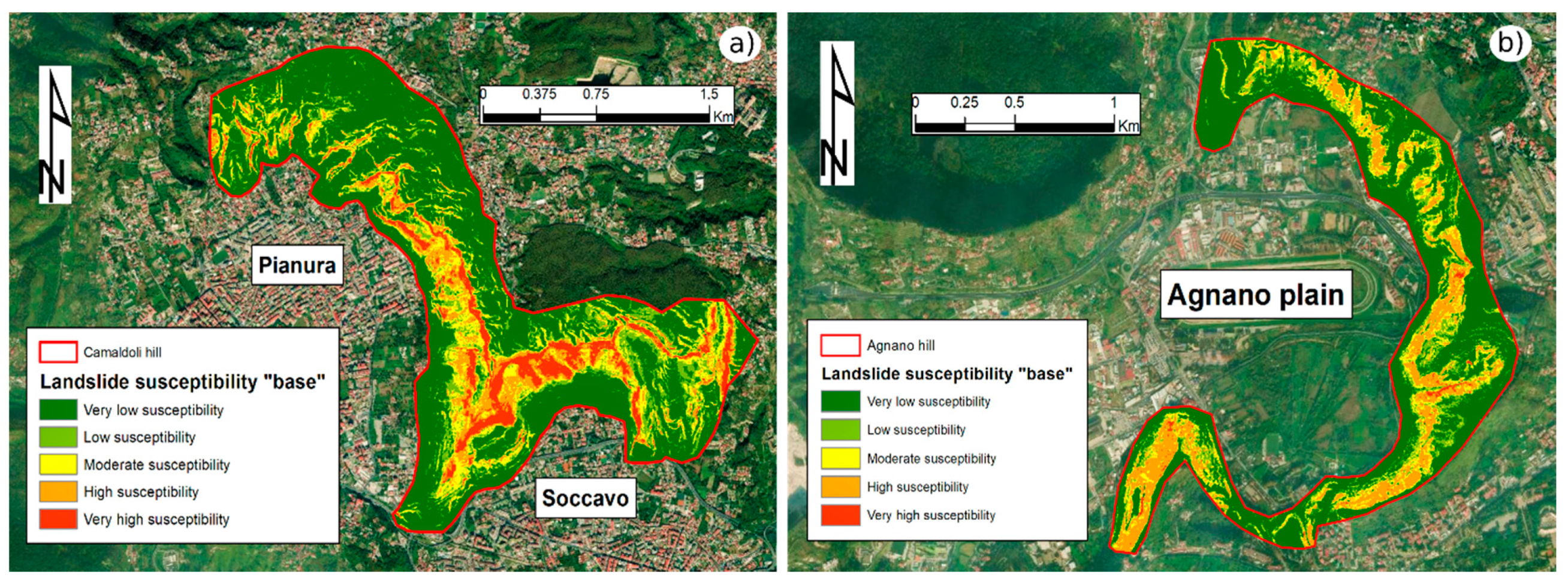
To quantify similarities and differences between the outcomes, such maps were divided into five susceptibility classes (I—very low susceptibility; II—low susceptibility; III—moderate susceptibility; IV—high susceptibility; V—very high susceptibility) using the Natural Breaks statistical classification (NBsc), which is based on the “optimization method” of [106]. NBsc aims to determine the best data distribution in significant classes, taking advantage of the intervals naturally present in the distributions of data and trying to minimize the variance within each class and maximizing that between the classes themselves. NBsc is undoubtedly an advantage because it allows the identification of groups of cells with homogeneous behaviour. Figure 5 shows the “base” susceptibility maps of the study area that represent the ensemble weighted average of the different models obtained individually.
The landslide susceptibility maps obtained from the ensemble method provide evidence that the largest part of the study area (70% Camaldoli—60% Agnano) has very low and low susceptibility to landslide occurrence, while 13% Camaldoli and 15% Agnano of the area has medium susceptibility to landslide occurrence. Lastly, the high and very high susceptibility classes cover 18% Camaldoli and 25% Agnano of the area (Figure 6b,d). The spatial aggregation of these susceptibility maps confirmed that the majority of the study region has a low susceptibility to the occurrence of landslide events. Therefore, the highest concentration of landslides can be found within the highest susceptibility class value (85% Camaldoli—90% Agnano) (Figure 6a,c). Moreover, the landslide distribution is characterized by an increasing trend when passing from the lowest to the highest classes of susceptibility. These considerations highlight that despite the limited area extension of the very high susceptibility class, most of the landslides surveyed fall within the latter. Such analyses confirmed the high performance of the models.
The accuracy of the different maps obtained was tested using receiver operating characteristic (ROC) curves, while true skill statistics (TSS) was used as an alternative measure of accuracy. The ROC curve is a frequently used method to present the results of binary classification between the outcomes of a predictive model (or classifier) and the actual occurrence of the forecasted event [107]. If a model predicts a positive value of a given variable (event forecast) and the value of the variable is positive (event), a true positive (TP) prediction is obtained. At the opposite, if the value of the variable is negative (no event), a false positive (FP) prediction is obtained. The ideal classifier should return a TP rate of 1 and an FP rate of 0, meaning it predicted all the events with no false alarm. The discriminant capacity of a model prediction can be assessed based on the area under the curve (AUC), included in the range 0 to 1 [108]. AUC values lower than 0.5 indicate insufficient performance, whereas models with AUC values of 0.7–0.8 indicate a very good performance [109,110]. The true skill statistic is the difference between the hit rate and the false alarm rate. It ranges between -1 and 1 and its best value is 1, not being affected by prevalence, differently from Kappa [111]. A TSS equal to −1 indicates that the model provides no better results than a random model.
A TSS equal to 0 indicates an indiscriminate model. Values ranging from 0.2 to 0.5 were considered poor, from 0.6 to 0.8 useful, and values larger than 0.8 were considered good to excellent [112]. Since TSS showed high-performance values, it was chosen to perform statistical analysis. Such percentages are summarized in Table 6.
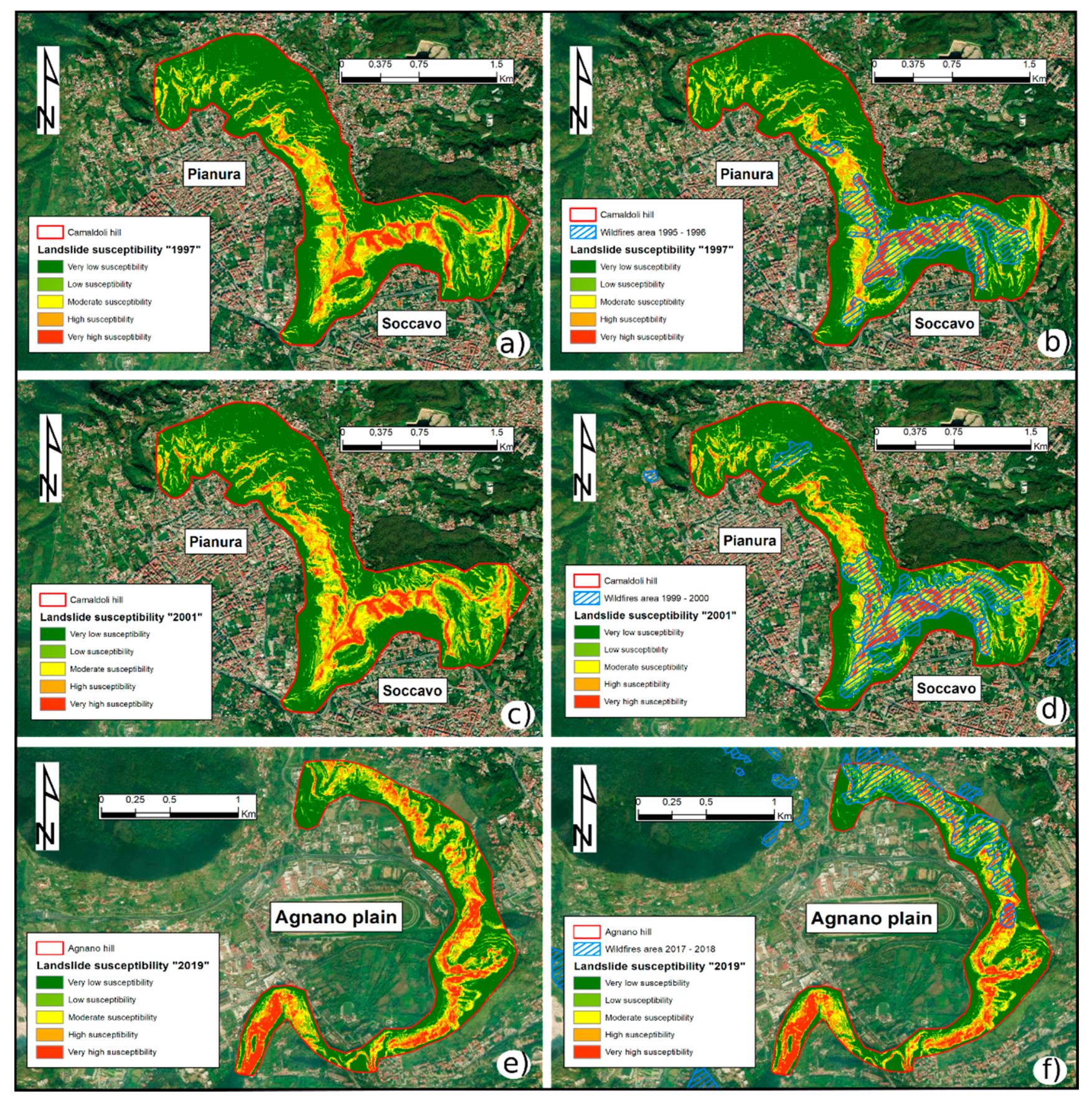
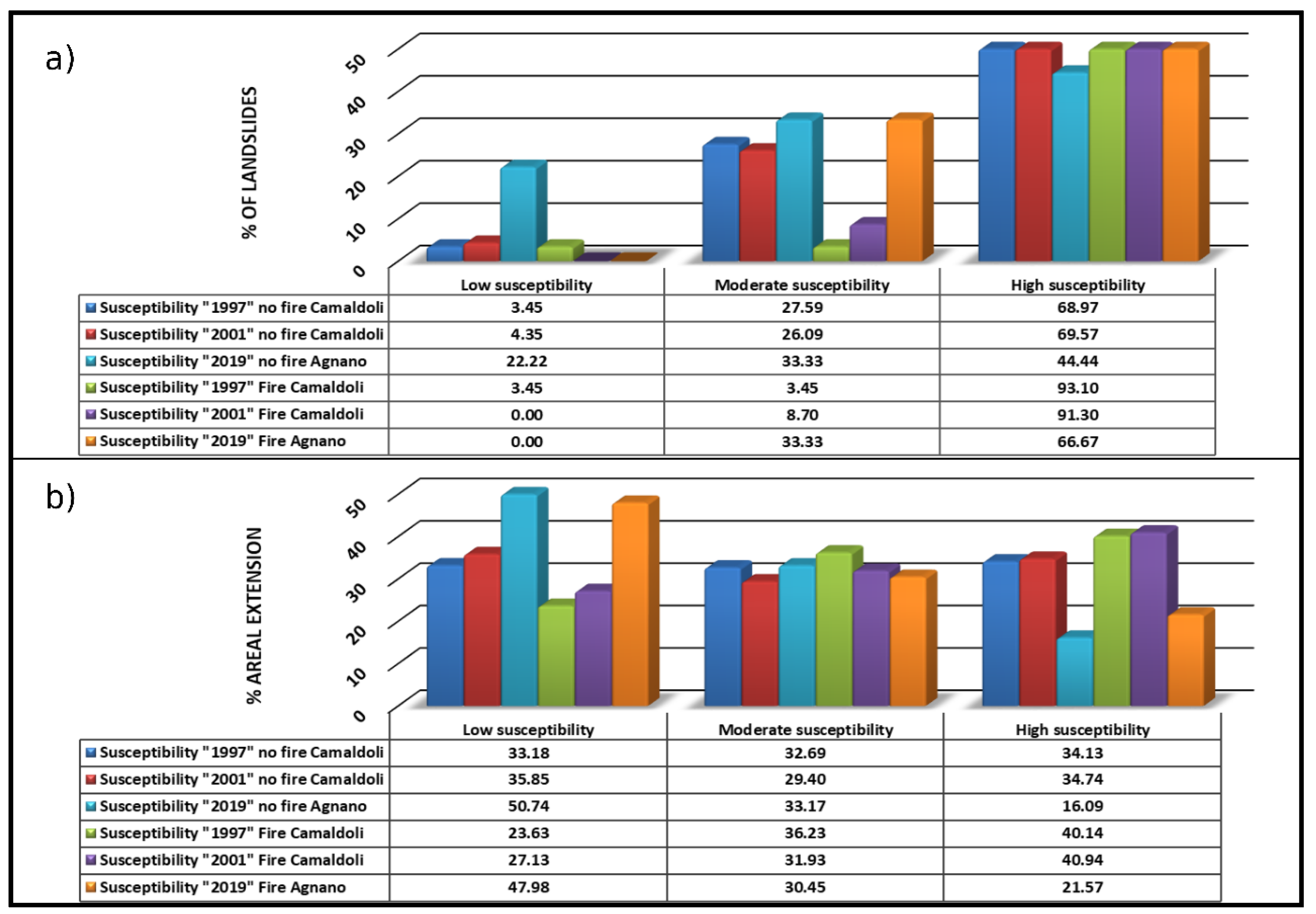
After obtaining the two “base” susceptibility maps for the study area, similar analyses were carried out, considering in this case all the predisposing factors analysed previously and adding the information on the portions affected by the wildfires. The results obtained are illustrated in Figure 7. Additionally, in this case, statistical analyses were carried out to make comparisons, since, visually, it is not possible to appreciate the differences with the maps previously obtained.
To compare the results, the maps obtained were first categorized in different susceptibility classes. Subsequently, an intersection operation between the output maps and the landslides surveyed was performed to acquire further information and to evaluate the distribution of landslides in the different susceptibility classes, and to define the areal distribution that they assume. Additionally, on this occasion, as previously underlined, it is possible to notice an increasing trend for landslides that fall in the most susceptible areas and a decreasing trend for the areal extension (Figure 8). The study of the aforementioned trends can represent a precise and rapid evaluation of the reliability of the models obtained. In fact, despite the areal extension of the higher susceptible class being extremely low, most landslides fall within it. Therefore, the implemented models were able to identify the areas most prone to future triggers of rainfall-induced landslides in a fairly coherent way. Furthermore, in the susceptibility maps in which the wildfire predisposing factor was considered, it has to be noted that the percentage of landslides with low susceptibility (classes I-II) shows values close to zero. This is most likely due to the worsening role that wildfires took on when the various modelling analyses were implemented. For this reason, many portions of the study area, which with the “base” maps had a lower susceptibility, assumed higher trigger probability values. Equally, this shifted some landslides into higher levels of susceptibility. This migration, in the classes with higher susceptibility, confirms the burden that wildfires confer on the slopes, making them more likely to trigger to areal erosion phenomena.
Furthermore, to validate all the hypotheses formulated, the pre- and post-fire susceptibility maps were compared with the landslides triggered in the burnt areas (Figure 9a) by estimating the area distribution of the different susceptibility classes (Figure 9b). The first operation was to select from the landslide database only those that triggered simultaneously and/or after the wildfires considered for the years in which the frequency of instability phenomena was high (1997, 2001, and 2019). To facilitate understanding, the susceptibility classes were combined into three classes: Low susceptibility (class I-II), moderate susceptibility (class III), and high susceptibility (class IV-V).
The selected landslides were intersected with the “base” susceptibility maps and with those developed for the years examined (1997, 2001, 2019). It is noted that in the class with low susceptibility, the presence of landslides is minimal if not absent. Considering, however, the class with high susceptibility, the presence of such phenomena tends to increase. Regarding the burnt areas as a predisposing factor, landslides tend to migrate in the moderate- and high-susceptibility classes. For example, considering the event in 2001, it is observed that in the least susceptible class the presence of landslides is equal to about 4%, in the middle class at 26%, and in the most susceptible class at 70%. Therefore, considering wildfires as a predisposing factor in the susceptibility analysis, the following percentage distribution of landslides is noted: In the least susceptible class, complete absence of landslides; in the intermediate class, 8%; and in the most susceptible class, 91% of the aforementioned phenomena (Figure 8a). This type of analysis allowed confirmation of the weight that this new variable has in the final model evaluation, and, as in all the study area, landslides tend to concentrate in the most susceptible areas. The same trend, even with different percentages, is observable when the areal extension was examined (Figure 8b). Additionally, in this case, the most susceptible classes have a higher percentage of propensity to trigger than the same class without considering the burnt areas.
It can, therefore, be said that this study allowed us to demonstrate quantitatively how the variable “wildfires” increase the propensity to trigger the phenomena considered. Lastly, another significant result is the importance of the variables function, which can assist in understanding the contribution of environmental predictors to the model outputs. This procedure uses a machine learning approach, where the principle is to shuffle a single variable of the given data. Model prediction with this ‘shuffled’ dataset was made. Then, a simple correlation was computed (Pearson’s by default) between the reference predictions and the ‘shuffled’ one. The returned score was 1-cor (predicted reference, predicted shuffled). A good correlation score between two predictors means that one of the two variables has a low influence and it is considered not important for the model. On the contrary, a low correlation means that both variables have a high influence on the model (Table 7). It has to be noted that this technique does not account for interactions between variables, but every variable must be considered individually and should be considered more as an information tool for each model independently [113].
In all models, the slope angle assumes a fundamental role in the final landslide susceptibility, confirming that such an environmental variable played a principal role in predicting landslide susceptibility within each model. Furthermore, it is noted that the wildfire areas also exhibited a significant score in the final evaluation, demonstrating that this predictor contributes to the final assessment. The rank order of variable importance was often irregular when comparing the different models. Yet, the highest-ranked factors were generally consistent. Other variables, such as TPI, land use, drainage density, and geo-lithology, show noteworthy values in almost all ensemble models. However, the different ranking of the variables’ importance between different machine learning techniques should be expected [82]. Additionally, one of the main shortcomings of the machine learning method is its simplistic approach to assess landslide susceptibility using a landslide inventory database (i.e., by simply including the point features) but discarding information on their shape and dimensions [114].

7. Discussion

Mapping the spatial prediction of wildfire susceptibility is an essential component of a variety of actions, such as emergency land management, wildfire prevention, and mitigation of fire impacts [29]. In this work, a study was conducted on landslides affecting the Camaldoli and Agnano hills, Naples, following two objectives in parallel: The processing of the thematic maps of the burnt areas through band compositions of satellite images, and landslide susceptibility assessment using machine learning techniques, improving the knowledge of the relationship between the triggering of landslides and burnt areas. The activity carried out for the database construction allowed the identification and digitalization of the entire study area, in the GIS environment, for the areas covered by fire referring to the dates of the fires that occurred from 1995 to 2019. The method used allowed very accurate digitization of all the events that occurred. The landslide susceptibility assessment is extremely influenced by the quality of the basic data available for the territory considered. In fact, to optimize the results, the analysis was implemented starting from a high-resolution DTM (5 m × 5 m), carrying out a fairly detailed analysis. Concerning the failure susceptibility, as predisposing factors, for which there are no universally recognized guidelines, the following parameters were chosen: Slope angle, slope aspect, profile curvature, planform curvature, distance to streams, streams density, geo-lithological map, topographic wetness index (TWI), topographic position index (TPI), land use, and wildfires, which are considered to correlate more with the type of susceptibility considered in the study area. In the first analysis, as regards the evaluation of the susceptibility to detachment, the “base” susceptibility map was drawn up (Figure 5) to understand the propensity shown without considering the role of wildfires. From the analyses carried out, it is clear that almost all the landslides fall into the most susceptible classes and their areal extension tends to assume a decreasing trend from the lower to the higher susceptibility classes. The results obtained indicate the good predictive ability of the methods used in identifying potentially unstable areas. In addition, the analyses carried out have a fairly high level of detail, managing to discretely disclose the different probabilities of occurrence. From the study of the scientific literature, developed in recent decades, a relationship between geomorphic processes and the occurrence of fires emerged, and on the contrary, the potential of the activity of areal, linear, and punctual erosion phenomena decreases with time and coincident revegetation. Precisely, most of the landslide processes occurred during the first rainy season after the fire or within one or two years after the fire [16,18,21,60]. For these reasons, susceptibility maps were implemented for the years 1997, 2001, and 2019 (Figure 7), knowing that the wildfires seem to have reacted as a predisposing factor to landslides that occurred in the same year, while the triggering factor is represented by rainfall [13]. To carry out this processing, the predisposing factors used for the susceptibility of the “base” were considered by adding the fires that occurred in the two years preceding the triggering instability phenomena. The data, the result of the statistical processing, were compared with those of the “base” susceptibility maps (Figure 8). The analysis of the data showed that considering the burnt areas (1995–1996; 1999–2000; 2017–2018) as an additional predisposing factor for the evaluation of the susceptibility analysis referring respectively to 1997, 2001, and 2019, there was an increase in susceptible areas compared to the “base” susceptibility and an increase in the percentage of landslides falling in the classes with higher susceptibility. This can be understood as fires represent an unfavourable role in the final susceptibility assessment, increasing the predisposition to the instability of the whole territory.

8. Conclusions

In conclusion, this work allowed landslide susceptibility assessment along the slopes of the Camaldoli and Agnano hills, considering also the burnt areas, the identification and digitization of which required a separate phase compared to that of the processing of the maps referring to other predisposing factors. The analysis of the data showed that considering the wildfire as a new conditioning factor, the predisposition to instability in the area has increased. The results obtained could be further improved by considering additional predisposing parameters but also triggering parameters, such as rainfalls. Besides, the study could be improved with an accurate scale analysis of the areas covered by fire, examining the variation of geotechnical characteristics of the material concerned before wildfire and subsequently involved in a landslide phenomenon. By setting up a classification scheme of the degree of decay of geotechnical characteristics of the geological material involved according to wildfire type (depending on the maximum temperature reached on the ground and the fire duration), it would be possible to obtain an even more realistic susceptibility forecast. Therefore, since the spatial prediction of wildfire susceptibility maps can illustrate the location of the element at risk, wildfire risk maps can be produced by considering the vulnerable areas in our case study.
Consequently, the maps drawn up in 1997, 2001, and 2019 could be considered in terms of hazard, being characterized by a time limit. These studies, of which this work represents an example, are not simply scientific speculation, being instead intended as a support for more effective territory management, more necessary than ever in a densely urbanized and morphologically articulated reality, such as that of the city of Naples.

Author Contributions

Conceptualization, D.D.M., M.R., S.L.U.; methodology, M.D.N., P.M.; software, M.D.N., P.M.; validation, M.D.N., P.M., D.D.M.; resources, data curation, M.D.N, P.M.; writing—original draft preparation, M.D.N., P.M., D.D.M.; writing—review and editing, M.R., S.L.U., D.C.; supervision, D.C. All authors have read and agreed to the published version of the manuscript.

Funding

This research received no external funding.

Acknowledgments

The authors would like to thank Serena Tessitore for her suggestions and comments, and Consorzio interUniversitario per la prevenzione dei Grandi Rischi (CUGRI) for providing hardware support. In addition, the authors would like to thank the anonymous reviewers for their valuable and insightful suggestions to improve the paper.

Conflicts of Interest

The authors declare no conflict of interest.

References

  1. Calcaterra, D.; de Riso, R.; Evangelista, A.; Nicotera, M.V.; Santo, A.; Scotto Di Santolo, A. Slope instabilities of the pyroclastic deposits in the Phlegraean district and in the carbonate Apennine (Campania, Italy). In Proceedings of the Workshop on Occurrence and Mechanisms of Flows in Natural Slopes and Earth-fills, Sorrento, Italy, 14–16 May 2003. [Google Scholar]
  2. Trigila, A.; Frattini, P.; Casagli, N.; Catani, F.; Crosta, G.; Esposito, C.; Iadanza, C.; Lagomarsino, D.; Mugnozza, G.S.; Segoni, S.; et al. Landslide Susceptibility Mapping at National Scale: The Italian Case Study. In Landslide Science and Practice: Volume 1: Landslide Inventory and Susceptibility and Hazard Zoning; Margottini, C., Canuti, P., Sassa, K., Eds.; Springer: Berlin/Heidelberg, Germany, 2013; pp. 287–295. ISBN 978-3-642-31325-7. [Google Scholar]
  3. Segoni, S.; Tofani, V.; Rosi, A.; Catani, F.; Casagli, N. Combination of Rainfall Thresholds and Susceptibility Maps for Dynamic Landslide Hazard Assessment at Regional Scale. Front. Earth Sci. 2018, 6, 85. [Google Scholar] [CrossRef] [Green Version]
  4. Lombardo, L.; Mai, P.M. Presenting logistic regression-based landslide susceptibility results. Eng. Geol. 2018, 244, 14–24. [Google Scholar] [CrossRef]
  5. Cannon, S.H.; DeGraff, J. The Increasing Wildfire and Post-Fire Debris-Flow Threat in Western USA, and Implications for Consequences of Climate Change. In Landslides—Disaster Risk Reduction; Sassa, K., Canuti, P., Eds.; Springer: Berlin/Heidelberg, Germany, 2009; pp. 177–190. ISBN 978-3-540-69970-5. [Google Scholar]
  6. Nyman, P.; Sheridan, G.J.; Smith, H.G.; Lane, P.N.J. Evidence of debris flow occurrence after wildfire in upland catchments of south-east Australia. Geomorphology 2011, 125, 383–401. [Google Scholar] [CrossRef]
  7. Tien Bui, D.; Pradhan, B.; Lofman, O.; Revhaug, I. Landslide Susceptibility Assessment in Vietnam Using Support Vector Machines, Decision Tree, and Naïve Bayes Models. Available online: https://www.hindawi.com/journals/mpe/2012/974638/ (accessed on 18 May 2020).
  8. Di Martire, D.; De Rosa, M.; Pesce, V.; Santangelo, M.A.; Calcaterra, D. Landslide hazard and land management in high-density urban areas of Campania region, Italy. Nat. Hazards Earth Syst. Sci. 2012, 12, 905–926. [Google Scholar] [CrossRef] [Green Version]
  9. Pham, B.T.; Tien Bui, D.; Prakash, I.; Dholakia, M.B. Hybrid integration of Multilayer Perceptron Neural Networks and machine learning ensembles for landslide susceptibility assessment at Himalayan area (India) using GIS. Catena 2017, 149, 52–63. [Google Scholar] [CrossRef]
  10. Lombardo, L.; Opitz, T.; Huser, R. Point process-based modeling of multiple debris flow landslides using INLA: An application to the 2009 Messina disaster. Stoch Environ. Res. Risk Assess. 2018, 32, 2179–2198. [Google Scholar] [CrossRef] [Green Version]
  11. Scaramella, M. The Case of Naples, Italy, in Understanding Slums: Case Studies for the Global Report 2003, United Nations Human Settlements Programme, 21. Available online: http://www.ucl.ac.uk/dpu-projects/GlobalReport/home.htm (accessed on 18 May 2020).
  12. Totaro, F.; Alberico, I.; Di Martire, D.; Nunziata, C.; Petrosino, P. The key role of hazard indices and hotspot in disaster risk management: The case study of Napoli and Pozzuoli municipalities (Southern Italy). J. Maps 2020, 16, 68–78. [Google Scholar] [CrossRef]
  13. Calcaterra, D.; Coppin, D.; de Vita, S.; Di Vito, M.A.; Orsi, G.; Palma, B.; Parise, M. Slope processes in weathered volcaniclastic deposits within the city of Naples: The Camaldoli Hill case. Geomorphology 2007, 87, 132–157. [Google Scholar] [CrossRef]
  14. Calcaterra, D.; Guarino, P.M. Dinamica morfologica e fenomeni franosi recenti nell’area collinare napoletana (settore occidentale). Geol. Tech. Ambient. 1999, 2, 11–17. [Google Scholar]
  15. Meyer, G.A.; Wells, S.G. Fire-related sedimentation events on alluvial fans, Yellowstone National Park, U.S.A. J. Sediment. Res. 1997, 67, 776–791. [Google Scholar] [CrossRef]
  16. Cannon, S.H. Debris-flow generation from recently burned watersheds. Environ. Eng. Geosci. 2001, 7, 321–341. [Google Scholar] [CrossRef]
  17. Conedera, M.; Peter, L.; Marxer, P.; Forster, F.; Rickenmann, D.; Re, L. Consequences of forest fires on the hydrogeological response of mountain catchments: A case study of the Riale Buffaga, Ticino, Switzerland. Earth Surf. Process. Landf. 2003, 28, 117–129. [Google Scholar] [CrossRef]
  18. Cannon, S.H.; Bigio, E.; Mine, E. A process for fire-related debris flow initiation, Cerro Grande fire, New Mexico. Hydrol. Process. 2001, 15, 3011–3023. [Google Scholar] [CrossRef]
  19. Swanson, F.J. Fire and geomorphic processes. Fire Regime and Ecosystem Properties. In General Technical Report WO; Mooney, H.A., Bonnicksen, T.M., Christiansen, N.L., Lotan, J.E., Reiners, W.A., Eds.; United States Departement of Agriculture, Forest Service: Washington, DC, USA, 1981; Volume 26, pp. 401–421. [Google Scholar]
  20. Moody, J.A.; Martin, D.A. Post-fire, rainfall intensity–peak discharge relations for three mountainous watersheds in the western USA. Hydrol. Process. 2001, 15, 2981–2993. [Google Scholar] [CrossRef]
  21. Cannon, S.H.; Gartner, J.E.; Parrett, C.; Parise, M. Wildfire-related debris flow generation through episodic progressive sediment bulking processes, western U.S.A. Debris-Flow Hazards Mitigation—Mechanics, Prediction, and Assessment. In Proceedings of the Third International Conference on Debris-Flow Hazards Mitigation, Davos, Switzerland, 10–12 September 2003; Rickenmann, D., Chen, C.L., Eds.; A.A. Balkema: Rotterdam, The Netherlands, 2003; pp. 71–82. [Google Scholar]
  22. DeBano, L.F. Fire’s effect on physical and chemical properties of chaparral soils. In Proceedings of the Symposium on the Environmental Consequences of Fire and Fuel Management in Mediterranean Ecosystems, Palo Alto, CA, USA, 1–5 August 1977; For. Serv. Gen. Tech. Report. pp. 65–74. [Google Scholar]
  23. Giovannini, G.; Lucchesi, S.; Giachetti, M. Effect of heating on some physical and chemical parameters related to soil aggregation and erodibility. Soil Sci. 1988, 146, 255–261. [Google Scholar] [CrossRef]
  24. Wells, W. Some Effects of Brushfires on Erosion Processes in Coastal Southern California. In Erosion and Sediment Transport in Pacific Rim Steeplands; Davies, T.R.H., Pearce, A.J., Eds.; January 1981, Chirst Church, New Zealand. Sponsored jointly by the Royal Society of New Zealand, New Zealand Hydrological Society, IAHS, and the National Water and Soil Conservation Authority of New Zealand; International Association of Hydrologic Sciences Publication: Wellington, New Zealand, 1981; Volume 132, pp. 305–342. [Google Scholar]
  25. Giovannini, G.; Lucchesi, S. Effect of fire on hydrophobic and cementing substances of soil aggregates. Soil Sci. 1983, 136, 231–236. [Google Scholar] [CrossRef]
  26. Cannon, S.H.; Reneau, S.L. Conditions for generation of fire-related debris flows, Capulin Canyon, New Mexico. Earth Surf. Process. Landf. 2000, 25, 1103–1121. [Google Scholar] [CrossRef]
  27. De Graff, J.V. A rationale for effective post-fire debris flow mitigation within forested terrain. Geoenviron Disasters 2018, 5, 7. [Google Scholar] [CrossRef]
  28. Tonini, M.; D’Andrea, M.; Biondi, G.; Degli Esposti, S.; Trucchia, A.; Fiorucci, P. A Machine Learning-Based Approach for Wildfire Susceptibility Mapping. The Case Study of the Liguria Region in Italy. Geosciences 2020, 10, 105. [Google Scholar] [CrossRef] [Green Version]
  29. Gholamnia, K.; Gudiyangada Nachappa, T.; Ghorbanzadeh, O.; Blaschke, T. Comparisons of Diverse Machine Learning Approaches for Wildfire Susceptibility Mapping. Symmetry 2020, 12, 604. [Google Scholar] [CrossRef] [Green Version]
  30. Esposito, G.; Esposito, E.; Matano, F.; Molisso, F.; Sacchi, M.; Porfido, S. Effects of a wildfireon rocks and soils in the Sarno Mountains, Campania, Southern Apennines. Rendiconti Online Soc. Geol. Ital. 2013, 24, 119–121. [Google Scholar]
  31. Calcaterra, D.; Parise, M.; Strumia, S.; Mazzella, E. Relations Between Fire, Vegetation and Landslides in the Heavily Populated Metropolitan Area of Naples, Italy. In Proceedings of the 1st North American Landslide Conference, Vail, CO, USA, 3–8 June 2007; Schaefer, V.R., Schuster, R.L., Turner, A.K., Eds.; Association of Environmental & Engineering Geologists: Denver, CO, USA, 2007; pp. 1448–1461. [Google Scholar]
  32. Addabbo, P.; Focareta, M.; Marcuccio, S.; Votto, C.; Ullo, S.L. Contribution of Sentinel-2 data for applications in vegetation monitoring. ACTA IMEKO 2016, 5, 44–54. [Google Scholar] [CrossRef]
  33. Addabbo, P.; Focareta, M.; Marcuccio, S.; Votto, C.; Ullo, S.L. Land cover classification and monitoring through multisensor image and data combination. In Proceedings of the 2016 IEEE International Geoscience and Remote Sensing Symposium (IGARSS), Beijing, China, 10–15 July 2016; pp. 902–905. [Google Scholar]
  34. Fiscante, N.; Focareta, M.; Galdi, C.; Ullo, S.L. Analysis and validation of high-resolution satellite DEMs generated from EROS-B data for montaguto landslide. In Proceedings of the 2012 IEEE International Geoscience and Remote Sensing Symposium, Munich, Germany, 22–27 July 2012; pp. 7549–7552. [Google Scholar]
  35. Cicala, L.; Angelino, C.V.; Fiscante, N.; Ullo, S.L. Landsat-8 and Sentinel-2 for fire monitoring at a local scale: A case study on Vesuvius. In Proceedings of the 2018 IEEE International Conference on Environmental Engineering (EE), Milan, Italy, 12–14 March 2018; pp. 1–6. [Google Scholar]
  36. Cicala, L.; Angelino, C.V.; Parrilli, S.; Fiscante, N.; Ullo, S.L.; Addabbo, P. Unsupervised Post-Fire Assessment of Burned Areas with Free and Open Multispectral Data Using OBIA. In Proceedings of the GEOBIA 2018–From Pixels to Ecosystems and Global Sustainability; Centre d’Etudes Spatiales de la BIOsphère (CESBIO) and Office National D’études et de Recherches Aérospatiales (ONERA) and Espace pour le Développement (ESPACE DEV) and Société T.E.T.I.S: Montpellier, France, 2018. [Google Scholar]
  37. Tien Bui, D. land cover change mapping using a combination of sentinel-1 data and multispectral satellite imagery: A case study of sanandaj county, kurdistan, Iran. Appl. Ecol. Environ. Res. 2019, 17, 5449–5463. [Google Scholar] [CrossRef]
  38. De Vivo, B.; Rolandi, G.; Gans, P.B.; Calvert, A.; Bohrson, W.A.; Spera, F.J.; Belkin, H.E. New constraints on the pyroclastic eruptive history of the Campanian volcanic Plain (Italy). Mineral. Petrol. 2001, 73, 47–65. [Google Scholar] [CrossRef]
  39. Deino, A.L.; Orsi, G.; de Vita, S.; Piochi, M. The age of the Neapolitan Yellow Tuff caldera-forming eruption (Campi Flegrei caldera–Italy) assessed by 40Ar/39Ar dating method. J. Volcanol. Geotherm. Res. 2004, 133, 157–170. [Google Scholar] [CrossRef]
  40. Orsi, G.; D’Antonio, M.; de Vita, S.; Gallo, G. The Neapolitan Yellow Tuff, a large-magnitude trachytic phreatoplinian eruption: Eruptive dynamics, magma withdrawal and caldera collapse. J. Volcanol. Geotherm. Res. 1992, 53, 275–287. [Google Scholar] [CrossRef]
  41. Orsi, G.; De Vita, S.; di Vito, M. The restless, resurgent Campi Flegrei nested caldera (Italy): Constraints on its evolution and configuration. J. Volcanol. Geotherm. Res. 1996, 74, 179–214. [Google Scholar] [CrossRef]
  42. Morra, V.; Calcaterra, D.; Cappelletti, P.; Colella, A.; Fedele, L.; De Gennaro, R.; Langella, A.; Mercurio, M.; De Gennaro, M. Urban geology: Relationships between geological setting and architectural heritage of the Neapolitan area. J. Virtual Explor. 2010, 36, 1–59. [Google Scholar] [CrossRef]
  43. Pappalardo, L.; Civetta, L.; D’Antonio, M.; Deino, A.; Di Vito, M.; Orsi, G.; Carandente, A.; de Vita, S.; Isaia, R.; Piochi, M. Chemical and Sr-isotopical evolution of the Phlegraean magmatic system before the Campanian Ignimbrite and the Neapolitan Yellow Tuff eruptions. J. Volcanol. Geotherm. Res. 1999, 91, 141–166. [Google Scholar] [CrossRef]
  44. Fedele, F.G.; Giaccio, B.; Isaia, R.; Orsi, G. The Campanian Ignimbrite Eruption, Heinrich Event 4, and Palaeolithic Change in Europe: A High-Resolution Investigation. In Volcanism and the Earth’s Atmosphere; American Geophysical Union (AGU): Naples, Italy, 2013; pp. 301–325. ISBN 978-1-118-66854-2. [Google Scholar]
  45. Scarpati, C.; Perrotta, A.; Sparice, D. Volcanism in the city of Naples. Rendicondi Online Soc. Geol. Ital. 2015, 33, 88–91. [Google Scholar] [CrossRef]
  46. Shakesby, R.A.; Doerr, S.H. Wildfire as a hydrological and geomorphological agent. Earth Sci. Rev. 2006, 74, 269–307. [Google Scholar] [CrossRef]
  47. Whelan, R.J. The Ecology of Fire; Cambridge University Press: Cambridge, UK, 1995. [Google Scholar]
  48. Neary, D.G.; Klopatek, C.C.; DeBano, L.F.; Ffolliott, P.F. Fire effects on belowground sustainability: A review and synthesis. For. Ecol. Manag. 1999, 122, 51–71. [Google Scholar] [CrossRef]
  49. Prosser, I. Fire, Humans and Denudation at Wangrah Creek, Southern Tablelands, N.S.W. Aust. Geograph. Stud. 1990, 28, 77–95. [Google Scholar] [CrossRef]
  50. Inbar, M.; Tamir, M.; Wittenberg, L. Runoff and erosion processes after a forest fire in Mount Carmel, a Mediterranean area. Geomorphology 1998, 24, 17–33. [Google Scholar] [CrossRef]
  51. Neary, D.G.; Ryan, K.C.; DeBano, L.F. (Eds.) Wildland Fire Inecosystems: Effects of Fire on Soils and Water; revised 2008. In General Technical Report RMRS-GTR-42; U.S. Department of Agriculture, Forest Service, Rocky Mountain Research Station: Ogden, UT, USA, 2005; Volume 4, 250p. [Google Scholar]
  52. Giovannini, G.; Lucchesi, S. Effects of Fire on Soil Physico-Chemical Characteristics and Erosion Dynamics. In Fire in Mediterranean Ecosystems; Trabaud, L., Prodon, R., Eds.; Commission of the European Communities: Brussels, Belgium, 1993; pp. 403–412. [Google Scholar]
  53. Giovannini, G.; Lucchesi, S. Modifications induced in soil physico-chemical parameters by experimental fires at different intensities. Soil Sci. 1997, 162, 479–486. [Google Scholar] [CrossRef]
  54. Wondzell, S.M.; King, J.G. Postfire erosional processes in the Pacific Northwest and Rocky Mountain regions. For. Ecol. Manag. 2003, 178, 75–87. [Google Scholar] [CrossRef]
  55. Savage, S.M. Mechanism of Fire-Induced Water Repellency in Soil. Soil Sci. Soc. Am. J. 1974, 38, 652–657. [Google Scholar] [CrossRef]
  56. Franco, C.M.M.; Clarke, P.J.; Tate, M.E.; Oades, J.M. Hydrophobic properties and chemical characterisation of natural water repellent materials in Australian sands. J. Hydrol. 2000, 231–232, 47–58. [Google Scholar] [CrossRef]
  57. Chandler, C.; Cheney, P.; Thomas, P.; Trabaud, L.; Williams, D. Fire in Forestry. Volume 1. Forest Fire Behavior and Effects. Volume 2. Forest Fire Management and Organization; John Wiley & Sons: New York, NY, USA, 1983. [Google Scholar]
  58. De Bano, L.F. The effects of fire on soil properties. For. Soils 1981, 151–155. [Google Scholar]
  59. Marxer, P.; Conedera, M. Experimental Fire in Switzerland. Final Report of the Prometheus System Validation Project; EU Project No. PL971037; Swiss Federal Research Institute, Sottostazione Sud delle Alpi: Bellinzona, Switzerland, 2000. [Google Scholar]
  60. Gartner, J.E.; Bigio, E.R.; Cannon, S.H. Compilation of Post Wildfire Runoff-Event Data from the Western United States; Open-File Report, 04-1085; United States Geological Survey: Reston, VA, USA, 2004. [CrossRef]
  61. Zavala, L.M.; Jordán, A.; Gil, J.; Bellinfante, N.; Pain, C. Intact ash and charred litter reduces susceptibility to rain splash erosion post-wildfire. Earth Surf. Process. Landf. 2009, 34, 1522–1532. [Google Scholar] [CrossRef]
  62. Zavala, L.M.M.; de Celis Silvia, R.; López, A.J. How wildfires affect soil properties. A brief review. Cuadernos de Investig. Geográfica/Geograph. Res. Lett. 2014, 40, 311–331. [Google Scholar] [CrossRef] [Green Version]
  63. Santi, P.M.; Morandi, L. Comparison of debris-flow volumes from burned and unburned areas. Landslides 2013, 10, 757–769. [Google Scholar] [CrossRef]
  64. DeGraff, J.V.; Cannon, S.H.; Gartner, J.E. The Timing of Susceptibility to Post-Fire Debris Flows in the Western United StatesPost-fire Debris Flow Timing. Environ. Eng. Geosci. 2015, 21, 277–292. [Google Scholar] [CrossRef]
  65. Staley, D.M.; Negri, J.A.; Kean, J.W.; Laber, J.L.; Tillery, A.C.; Youberg, A.M. Prediction of spatially explicit rainfall intensity–duration thresholds for post-fire debris-flow generation in the western United States. Geomorphology 2017, 278, 149–162. [Google Scholar] [CrossRef]
  66. van Westen, C.J.; Castellanos, E.; Kuriakose, S.L. Spatial data for landslide susceptibility, hazard, and vulnerability assessment: An overview. Eng. Geol. 2008, 102, 112–131. [Google Scholar] [CrossRef]
  67. Corominas, J.; van Westen, C.; Frattini, P.; Cascini, L.; Malet, J.-P.; Fotopoulou, S.; Catani, F.; Van Den Eeckhaut, M.; Mavrouli, O.; Agliardi, F.; et al. Recommendations for the quantitative analysis of landslide risk. Bull. Eng. Geol. Environ. 2014, 73, 209–263. [Google Scholar] [CrossRef]
  68. Finicelli, G.F.; Confuorto, P.; Carratù, M.T.; Di Martire, D. Multivariate Statistical approach vs. Deterministic physically based model for landslide susceptibility assessment. Rendicondi Online Soc. Geol. Ital. 2016, 41, 151–154. [Google Scholar] [CrossRef]
  69. Cruden, D.M.; Varnes, D.J. Landslides: Investigation and Mitigation; Chapter 3–Landslide Types and Processes. In Transport Research Board Special Report; Turner, K.A., Schuster, R.L., Eds.; The National Academies of Sciences, Engineering, and Medicine: Washington, DC, USA, 1996; Volume 247, pp. 36–75. [Google Scholar]
  70. Hungr, O. Review of the classification of landslides of the flow type. Environ. Eng. Geosci. 2001, 7, 221–238. [Google Scholar] [CrossRef]
  71. Kornejady, A.; Ownegh, M.; Bahremand, A. Landslide susceptibility assessment using maximum entropy model with two different data sampling methods. CATENA 2017, 152, 144–162. [Google Scholar] [CrossRef]
  72. Sadr, M.P.; Maghsoudi, A.; Saljoughi, B.S. Landslide susceptibility mapping of komroud sub-basin using Fuzzy logic approach. Proc. Geodynam. Res. Int. Bull. 2014, 2, XVI–XXVIII. [Google Scholar]
  73. Rahmati, O.; Pourghasemi, H.R.; Melesse, A.M. Application of GIS-based data driven random forest and maximum entropy models for groundwater potential mapping: A case study at Mehran Region, Iran. CATENA 2016, 137, 360–372. [Google Scholar] [CrossRef]
  74. Pourghasemi, H.R.; Pradhan, B.; Gokceoglu, C. Application of fuzzy logic and analytical hierarchy process (AHP) to landslide susceptibility mapping at Haraz watershed, Iran. Nat. Hazards 2012, 2, 965–996. [Google Scholar] [CrossRef]
  75. Beven, K.J.; Kirby, M.J. A physically based, variable contributing area model of basin hydrology. Hydrol. Sci. Bull. 1979, 24, 43–69. [Google Scholar] [CrossRef] [Green Version]
  76. Wilson, J.P.; Gallant, J.C. Digital terrain analysis. Terrain Anal. Princ. Appl. 2000, 6, 1–27. [Google Scholar]
  77. Shirzadi, A.; Bui, D.T.; Pham, B.T.; Solaimani, K.; Chapi, K.; Kavian, A.; Shahabi, H.; Revhaug, I. Shallow landslide susceptibility assessment using a novel hybrid intelligence approach. Environ. Earth Sci. 2017, 76, 60. [Google Scholar] [CrossRef]
  78. Barlow, J.; Martin, Y.; Franklin, S.E. Detecting translational landslide scars using segmentation of Landsat ETM+ and DEM data in the northern Cascade Mountains, British Columbia. Can. J. Remote Sens. 2003, 29, 510–517. [Google Scholar] [CrossRef]
  79. Chen, W.; Moriya, K.; Sakai, T.; Koyama, L.; Cao, C.X. Mapping a burned forest area from Landsat TM data by multiple methods. Geom. Nat. Hazards Risk 2016, 7, 384–402. [Google Scholar] [CrossRef] [Green Version]
  80. Congedo, L. Semi-Automatic Classification Plugin Documentation. Release 2016, 4, 29. [Google Scholar]
  81. Yalcin, A.; Reis, S.; Aydinoglu, A.C.; Yomralioglu, T. A GIS-based comparative study of frequency ratio, analytical hierarchy process, bivariate statistics and logistics regression methods for landslide susceptibility mapping in Trabzon, NE Turkey. CATENA 2011, 85, 274–287. [Google Scholar] [CrossRef]
  82. Goetz, J.N.; Brenning, A.; Petschko, H.; Leopold, P. Evaluating machine learning and statistical prediction techniques for landslide susceptibility modeling. Comput. Geosci. 2015, 81, 1–11. [Google Scholar] [CrossRef]
  83. Sepe, C.; Confuorto, P.; Angrisani, A.C.; Di Martire, D.; Di Napoli, M.; Calcaterra, D. Application of a Statistical Approach to Landslide Susceptibility Map Generation in Urban Settings. In IAEG/AEG Annual Meeting Proceedings, San Francisco, California, 2018–Volume 1; Shakoor, A., Cato, K., Eds.; Springer International Publishing: Cham, Switzerland, 2019; pp. 155–162. [Google Scholar]
  84. Xiao, T.; Yin, K.; Yao, T.; Liu, S. Spatial prediction of landslide susceptibility using GIS-based statistical and machine learning models in Wanzhou County, Three Gorges Reservoir, China. Acta Geochim. 2019, 38, 654–669. [Google Scholar] [CrossRef]
  85. Segoni, S.; Lagomarsino, D.; Fanti, R.; Moretti, S.; Casagli, N. Integration of rainfall thresholds and susceptibility maps in the Emilia Romagna (Italy) regional-scale landslide warning system. Landslides 2015, 12, 773–785. [Google Scholar] [CrossRef] [Green Version]
  86. Lombardo, L.; Bachofer, F.; Cama, M.; Märker, M.; Rotigliano, E. Exploiting Maximum Entropy method and ASTER data for assessing debris flow and debris slide susceptibility for the Giampilieri catchment (north-eastern Sicily, Italy). Earth Surf. Process. Landf. 2016, 41, 1776–1789. [Google Scholar] [CrossRef] [Green Version]
  87. Carotenuto, F.; Angrisani, A.C.; Bakthiari, A.; Carratù, M.T.; Di Martire, D.; Finicelli, G.F.; Raia, P.; Calcaterra, D. A New Statistical Approach for Landslide Susceptibility Assessment in the Urban Area of Napoli (Italy). In Workshop on World Landslide Forum; Mikos, M., Tiwari, B., Yin, Y., Sassa, K., Eds.; Springer International Publishing: Cham, Switzerland, 2017; pp. 881–889. [Google Scholar]
  88. Di Napoli, M.; Carotenuto, F.; Cevasco, A.; Confuorto, P.; Di Martire, D.; Firpo, M.; Pepe, G.; Raso, E.; Calcaterra, D. Machine learning ensemble modelling as a tool to improve landslide susceptibility mapping reliability. Landslides 2020, 17, 1897–1914. [Google Scholar] [CrossRef]
  89. The R Project for Statistical Computing R: A Language and Environment for Statistical Computing. Available online: https://www.r-project.org/ (accessed on 19 May 2020).
  90. Elith, J.; Graham, C.H.; Anderson, R.P.; Dudík, M.; Ferrier, S.; Guisan, A.; Hijmans, R.J.; Huettmann, F.; Leathwick, J.R.; Lehmann, A.; et al. Novel methods improve prediction of species’ distributions from occurrence data. Ecography 2006, 29, 129–151. [Google Scholar] [CrossRef] [Green Version]
  91. Araújo, M.B.; Pearson, R.G.; Thuiller, W.; Erhard, M. Validation of species–climate impact models under climate change. Glob. Chang. Biol. 2005, 11, 1504–1513. [Google Scholar] [CrossRef] [Green Version]
  92. Thuiller, W.; Lafourcade, B.; Engler, R.; Araújo, M.B. BIOMOD—A platform for ensemble forecasting of species distributions. Ecography 2009, 32, 369–373. [Google Scholar] [CrossRef]
  93. Stokes, A.; Atger, C.; Bengough, A.G.; Fourcaud, T.; Sidle, R.C. Desirable plant root traits for protecting natural and engineered slopes against landslides. Plant Soil 2009, 324, 1–30. [Google Scholar] [CrossRef]
  94. Preti, F. Forest protection and protection forest: Tree root degradation over hydrological shallow landslides triggering. Ecol. Eng. 2013, 61, 633–645. [Google Scholar] [CrossRef]
  95. Vergani, C.; Giadrossich, F.; Buckley, P.; Conedera, M.; Pividori, M.; Salbitano, F.; Rauch, H.; Lovreglio, R.; Schwarz, M. Root reinforcement dynamics of European coppice woodlands and their effect on shallow landslides: A review. Earth Sci. Rev. 2017, 167, 88–102. [Google Scholar] [CrossRef]
  96. Meisina, C.; Bordoni, M.; Vercesi, A.; Maerker, M.; Ganimede, C.; Reguzzi, M.C.; Capelli, E.; Mazzoni, E.; Simoni, S.; Gagnarli, E. Effects of Vineyard Inter-Row Management on Soils, Roots and Shallow Landslides Probability in the Apennines, Lombardy, Italy. Proceedings 2019, 30, 41. [Google Scholar] [CrossRef] [Green Version]
  97. Sidle, R.C.; Dhakal, A.S. Potential effects of environmental change on landslide hazards in forest environments. Environ. Chang. Geomorph. Hazards For. 2002, 123–165. [Google Scholar]
  98. Ma, K.-C.; Lin, Y.-J.; Maa, S.-Y.; Tan, Y.-C. Evaluation of the effect of hysteretic flow and root system on shallow landslide. Soil Res. 2012, 50, 616–624. [Google Scholar] [CrossRef]
  99. Dias, A.S.; Pirone, M.; Urciuoli, G. Review on Types of Root Failures in Shallow Landslides. In Workshop on World Landslide Forum; Mikos, M., Tiwari, B., Yin, Y., Sassa, K., Eds.; Springer International Publishing: Cham, Switzerland, 2017; pp. 633–640. [Google Scholar]
  100. Amato, M.; Di Martino, P.; Di Pasquale, G.; Mazzoleni, S.; Migliozzi, A.; Strumia, S. Il ruolo della vegetazione nelle frane di Quindici. Quad. Geol. Appl. 2000, 7, 97–108. [Google Scholar]
  101. Tien Bui, D.; Bui, Q.-T.; Nguyen, Q.-P.; Pradhan, B.; Nampak, H.; Trinh, P.T. A hybrid artificial intelligence approach using GIS-based neural-fuzzy inference system and particle swarm optimization for forest fire susceptibility modeling at a tropical area. Agric. For. Meteorol. 2017, 233, 32–44. [Google Scholar] [CrossRef]
  102. Arabameri, A.; Pourghasemi, H.R.; Yamani, M. Applying different scenarios for landslide spatial modeling using computational intelligence methods. Environ. Earth Sci. 2017, 76, 832. [Google Scholar] [CrossRef]
  103. Arabameri, A.; Pradhan, B.; Lombardo, L. Comparative assessment using boosted regression trees, binary logistic regression, frequency ratio and numerical risk factor for gully erosion susceptibility modelling. CATENA 2019, 183, 104223. [Google Scholar] [CrossRef]
  104. Guisan, A.; Thuiller, W.; Zimmermann, N.E. Habitat Suitability and Distribution Models: With Applications in R; Cambridge University Press: Cambridge, UK, 2017; ISBN 978-0-521-76513-8. [Google Scholar]
  105. Hair, J.F.; Black, W.C.; Babin, B.J.; Anderson, R.E. Multivariate Data Analysis: A Global Perspective, 7th ed.; Pearson Education Inc.: New Jersey, NJ, USA, 2010. [Google Scholar]
  106. Jenks, G.F. The Data Model Concept in Statistical Mapping. International Yearbook of Cartography; University of Ulm: Ulm, Germany, 1967; Volume 7, pp. 186–190. [Google Scholar]
  107. Donner, R.V.; Barbosa, S.M. Nonlinear Time Series Analysis in the Geosciences: Applications in Climatology, Geodynamics and Solar-Terrestrial Physics; Springer: Berlin/Heidelberg, Germany, 2008. [Google Scholar]
  108. Swets, J.A. Measuring the accuracy of diagnostic systems. Science 1988, 240, 1285–1293. [Google Scholar] [CrossRef] [Green Version]
  109. Peterson, A.T.; Papeş, M.; Soberón, J. Rethinking receiver operating characteristic analysis applications in ecological niche modeling. Ecol. Model. 2008, 213, 63–72. [Google Scholar] [CrossRef]
  110. Corsini, A.; Mulas, M. Use of ROC curves for early warning of landslide displacement rates in response to precipitation (Piagneto landslide, Northern Apennines, Italy). Landslides 2017, 14, 1241–1252. [Google Scholar] [CrossRef]
  111. Allouche, O.; Tsoar, A.; Kadmon, R. Assessing the accuracy of species distribution models: Prevalence, kappa and the true skill statistic (TSS). J. Appl. Ecol. 2006, 43, 1223–1232. [Google Scholar] [CrossRef]
  112. Coetzee, B.W.T.; Robertson, M.P.; Erasmus, B.F.N.; Rensburg, B.J.V.; Thuiller, W. Ensemble models predict Important Bird Areas in southern Africa will become less effective for conserving endemic birds under climate change. Glob. Ecol. Biogeogr. 2009, 18, 701–710. [Google Scholar] [CrossRef]
  113. Thuiller, W.; Georges, D.; Engler, R.; Breiner, F. Biomod2: Ensemble platform for species distribution modeling. R Package Version 2016, 2, r560. [Google Scholar]
  114. Pourghasemi, H.R.; Rahmati, O. Prediction of the landslide susceptibility: Which algorithm, which precision? CATENA 2018, 162, 177–192. [Google Scholar] [CrossRef]
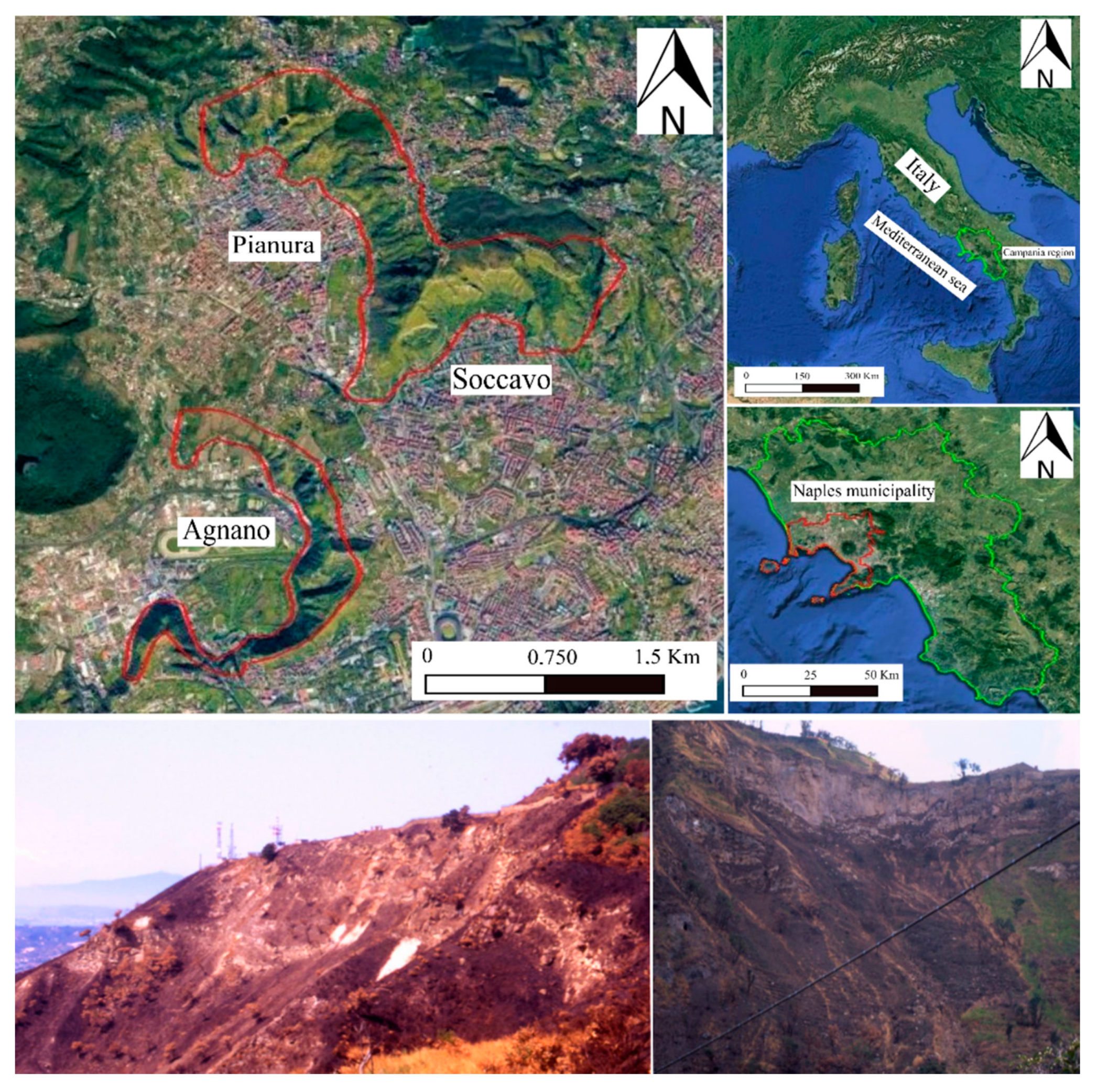
Figure 1. Location of the study area. In the top-left inset, the study area in detail; in red, the Camaldoli and Agnano hills. In the bottom-left inset, post-fire erosion phenomena (15 September 2001); in the bottom-right inset, the post-fire landslides triggered in the summer of 1996. Both images refer to the Soccavo slopes (photo: D. Calcaterra).
Remotesensing 12 02505 g001
Figure 2. Geological sketch map of the Naples municipality area. Caldera rims associated with two large Plinian and Phreatoplinian eruptions are also illustrated (CI and NYT) (modified after [45]).
Remotesensing 12 02505 g002
Figure 3. Flow chart of the implemented approach.
Remotesensing 12 02505 g003
Figure 4. (a,b) Pre- and post-fire conditions visible with a band composition 7-4-2; (c,d) pre- and post-fire conditions visible with a 7-5-3 band composition. In (b,d), red polygons are shown, which highlight where the wildfire occurred. Note that with the band composition 7-4-2, the identification of the burnt areas is more and evident than with the 7-5-3 band composition.
Remotesensing 12 02505 g004
Figure 5. “Base” ensemble susceptibility maps. (a) Weighted mean ensemble susceptibility map of the Camaldoli hill; (b) weighted mean ensemble susceptibility map of the Agnano hills.
Remotesensing 12 02505 g005
Figure 6. Landslide and areal extension distribution in susceptibility classes for the Agnano hills (a,b) and the Camaldoli hill (c,d).
Remotesensing 12 02505 g006
Figure 7. Landslide susceptibility maps considering also the burnt areas. (a,b) Susceptibility map considering fires that occurred in 1995–1996 and the rainfall-triggered landslides of 1997 (Camaldoli hill); (c,d) susceptibility maps considering the fires that occurred in 1999–2000 and the rainfall-triggered landslides of 2001 (Camaldoli hill); finally, (e,f) susceptibility map considering the fires that occurred in 2017–2018 and the rainfall-triggered landslides of 2019 (Agnano hills).
Remotesensing 12 02505 g007
Figure 8. (a) Landslide susceptibility distribution of wildfires area in the different classes; (b) areal extension distribution of susceptibility maps of the wildfire area for each susceptibility level.
Remotesensing 12 02505 g008
Figure 9. (a) Percentage of landslides falling in pre- and post-fire susceptibility maps; (b) percentage of pre- and post-fire areal extension.
Remotesensing 12 02505 g009
Table 1. Land-use types’ code description.
Land-Use Types CodeBrief Description
1Urbanized residential areas cover more than 80% of the total area.
2Urbanized residential areas made up of buildings and roads are between 80% and 30% of the total area.
3Areas occupied by buildings used for production activities, factory and commercial units.
4Areas covered by vegetation that reach the surface of 0.5 ha. This includes urban parks, municipal villas, public and private gardens.
5All sports areas are included in the class.
6Fruit trees and berry plantations.
7The class includes low productivity forage areas. They are often located in rough areas.
8Mosaic of land that cannot be individually mapped with various temporary crops, stable lawns and permanent crops, each occupying less than 50% of the total area.
9This class includes crops interrupted by natural forest areas of considerable size. Crops occupy more than 25 and less than 75% of the total area.
10Broad-leaved forest
11Sclerophyllous vegetation is a plant association of Mediterranean environments made up of trees with arboreal growth.
12This class is formed by shrub or herbaceous vegetation with scattered trees.
Table 2. Band composition chosen to combine the satellite images referring to the Landsat 4-5 constellation.
Landsat 4-5
Bands
Wavelength [micrometres]Resolution [meters]
Band 7—SWIR2.09–2.3530
Band 4—Near Infrared (NIR)0.77–0.9030
Band 2—Green0.52–0.6030
Table 3. Bands chosen for the composition of Sentinel-2 images.
Sentinel-2 BandsCentral Wavelength [μm]Resolution [m]
Band 3—Green0.56010
Band 4—Red0.66510
Band 6—Vegetation Red Edge0.74020
Band 7—Vegetation Red Edge0.78320
Band 11—SWIR1.61020
Band 12—SWIR2.19020
Table 4. Wildfires geodatabase from 1995 to 2019. Satellite imagery period = the data range within the satellite imagery was found for download; pre- and post-fire images = reference images (respectively pre- and post-fire) used for the digitization of burnt areas.
Camaldoli Hill
Search Period of Satellite ImagesFire DateYearPre- and Post-Fire ImagesSlope
01/06/1995_01/10199515/08/1995199528/07/1995_/29/08/1995Pianura
01/06/1995_01/10/199524/08/1995199528/07/1995_/29/08/1995Soccavo
01/08/1995_01/10/199512/09/1995199529/08/1995_30/09/1995Pianura
01/09/1995_01/12/199528/10/1995199523/10/1995_01/11/1995Soccavo
01/10/1995_01/07/199617/06/1996199601/11/1995_28/06/1996Pianura
01/06/1996_01/09/1996Summer199605/07/1996_14/07/1996Soccavo
01/06/1996_01/09/199626/07/1996199621/07/1996_06/08/1996Pianura
01/06/1996_01/09/199627/07/1996199621/07/1996_06/08/1996Soccavo
01/07/1997_01/09/199728/07/1997199708/07/1997_02/08/997Soccavo
01/07/1997_01/09/1997Summer199708/07/1997_02/08/997Pianura
01/08/1997_01/10/199715/08/1997199709/08/1997_26/091997Pianura
01/01/1998_01/03/1998Summer199825/01/1998_10/02/1998Pianura
01/07/199_01/08/199921/07/1999199905/06/1999_08/08/1999Soccavo
01/07/199_01/08/1999Summer199905/06/1999_08/08/1999Pianura
01/08/1999_01/10/1999Summer199924/08/1999_25/09/1999Soccavo
01/08/1999_01/10/199921/09/1999199924/08/1999_25/09/1999Pianura
01/06/2000_01/09/2000Summer200030/06/2000_01/08/2000Soccavo
01/06/2000_01/09/2000Summer200001/08/2000_11/09/2000Soccavo
01/06/2000_01/09/200003/08/2000200001/08/2000_11/09/2000Soccavo
01/06/2000_01/09/2000Summer200001/08/2000_11/09/2000Pianura
01/07/2001_01/09/200101/08/2001200128/07/2001_04/08/2001Soccavo
01/07/2003_01/10/200325/07/2003200318/07/203_03/08/2003Pianura
01/07/2003_01/10/200306/08/2003200303/08/2003_10/08/2003Pianura
01/07/2003_01/10/200311–13/08/2003200310/08/2003_19/08/2003Pianura
01/05/2007_01/11/200726/06/2007200718/06/2007_15/09/2007Soccavo
01/06/2007_01/11/200717/08/2007200718/06/2007_15/09/2007Pianura
01/05/2007_01/11/2007Summer200718/06/2007_15/06/2007Soccavo
01/05/2007_01/11/200706/09/2007200718/06/2007_15/09/2007Pianura
01/07/2009_01/10/200916/08/2009200910/08/2009_19/08/2009Soccavo
01/08/2011_01/11/201114/09/2011201110/09/2011_03/09/2001Soccavo
01/08/2011_01/11/201117/09/2011201110/09/2011_03/10/2011Soccavo
01/07/2013_01/10/201321/08/2013201305/08/2013_06/09/2013Soccavo
01/07/2013_01/10/2013Summer201305/08/2013_06/09/2013Soccavo
01/08/2015_01/04/201626/12/2015201517/12/2015_18/01/2016Pianura
01/04/2016_01/09/201623/07/2016201622/07/2016_04/08/2016Soccavo
01/04/2016_01/09/201617/08/2016201611/08/2016_03/09/2016Soccavo
01/05/2017_01/10/201718/06/2017201717/05/2017_20/06/2017Pianura
01/05/2017_01/10/201710/08/2017201706/08/2017_16/08/2017Pianura
01/05/2019_01/10/2019Summer201917/06/2019_23/10/2019Pianura
01/05/2019_01/10/2019Summer201917/06/2019_23/10/2019Soccavo
Agnano Plain
Search Period of Satellite ImagesFire DateYearPre- and Post-Fire ImagesSlope
01/05/2017_01/10/2017Summer201706/08/2017_16/08/2017Agnano
01/05/2018_01/10/2018Summer201802/06/2018_30/09/2018Agnano
01/05/2019_01/10/2019Summer201917/06/2019_23/10/2019Agnano
Table 5. Multicollinearity diagnosis indices for variables; such scores represent the mean of the different models implemented.
Multi-CollinearityVIFSTEPVIFCOR
Slope angle1.962.02
Slope aspect1.011.02
Profile curvature1.371.47
Planform curvature1.521.62
Stream density1.131.15
TWI2.342.26
TPI1.501.46
Distance to stream1.281.32
Geo-lithology1.361.41
Land Use1.141.15
Wildfire area1.391.48
Table 6. AUC/ROC and TSS scores for the ensemble models used.
AUC/ROCTSS
WMean Susceptibility “base”
Camaldoli
0.950.79
WMean Susceptibility “base”
Agnano
0.950.76
WMean Susceptibility “1997”
Camaldoli
0.960.79
WMean Susceptibility “2001”
Camaldoli
0.960.82
WMean Susceptibility “2019”
Agnano
0.950.84
Table 7. Variables’ importance for the ensemble models. Green columns refer to the ensemble methods applied without the wildfire variable, blue columns also include the wildfire variable.
Ensemble
Models
Wmean “Base” CamaldoliWmean “Base” AgnanoWmean “1997” CamaldoliWmean “2001” CamaldoliWmean “2019” Agnano
Slope angle0.760.740.650.770.76
Slope aspect0.020.0610.010.0290.048
Profile curvature0.0040.0070.0070.0060.005
Planform curvature0.0040.030.010.0110.036
Stream density0.110.0480.10.180.074
TWI0.020.0420.010.0190.025
TPI0.180.070.20.1430.094
Distance to river0.0010.0010.0010.0040.00002
Geo-lithology0.270.230.30.0320.176
Land Use0.0620.020.40.450.05
Wildfire area//0.210.30.192