Proof of Concept for Sea Ice Stage of Development Classification Using Deep Learning

Abstract

Accurate maps of ice concentration and ice type are needed to address increased interest in commercial marine transportation through the Arctic. RADARSAT-2 SAR imagery is the primary source of data used by expert ice analysts at the Canadian Ice Service (CIS) to produce sea ice maps over the Canadian territory. This study serves as a proof of concept that neural networks can be used to accurately predict ice type from SAR data. Datasets of SAR images served as inputs, and CIS ice charts served as labelled outputs to train a neural network to classify sea ice type. Our results show that DenseNet achieves the highest overall classification accuracy of 94.0% including water and the highest ice classification accuracy of 91.8% on a three class dataset using a fusion of HH and HV SAR polarizations for the input samples. The 91.8% ice classification accuracy validates the premise that a neural network can be used to effectively categorize different ice types based on SAR data.

1. Introduction

Sea ice is a central component of the Arctic cryosphere. It covers the Arctic Ocean on an annual basis and persists throughout the summer months as multiyear sea ice. In a time of a rapidly changing climate, there is a demand for local-scale high-resolution information on Arctic marine conditions (e.g., environmental conditions, sea ice state and dynamics) to support logistical operations, transportation, and sea ice use. From an industrial and transportation perspective, knowledge of the ever-changing state of sea ice conditions is critical for operations planning (e.g., Environment and Climate Change Canada Regional Ice-Ocean Prediction System [1]), shipping routes, and sustainable development of the North. During the summer season, changing sea ice conditions have led to changes in transportation and usage of Arctic waterways [2]. The reduction of sea ice has led to greater mobility and a higher level of unpredictability and risk [3]. Additionally, changing sea ice characteristics such as thickness, extent, type, and thermodynamic state collectively influence how energy transfers across the ocean/sea-ice/atmosphere (OSA) boundary. In the Arctic, sea ice influences radiative forcing and is a contributing factor to the heat budget of the planet. Therefore, knowledge of the physical and thermodynamic state of sea ice is critically important to understanding how climate change is affecting our world.

Satellite based synthetic aperture radar (SAR) systems are capable of measurements of the Earth’s surface in all weather conditions and in darkness. For these reasons, they are regularly used for monitoring the vast regions of the Arctic. There are many operational spaceborne SAR systems that regularly provide SAR imagery in the microwave C-band (5.5 GHz). Examples include the Canadian satellites RADARSAT-2 and RADARSAT Constellation Mission (RCM) and the European Space Agency’s Sentinel-1A and -1B. These systems have a high spatial resolution (e.g., below 100 m pixel spacing) and have regional coverage (e.g., up to 500 km by 500 km), making them ideal for monitoring large regions. Systems can operate in various acquisition modes (e.g., single polarization, HH; dual-polarization, HH and HV), with different polarization combinations yielding unique images of the region of interest. In simple terms, the processed output product of the imaging satellite SAR is a map of the normalized radar cross-section (NRCS, denoted as ${\sigma }^0$, with units of dB) that may contain regions of land, open water, and sea ice.

Within each satellite image, the microwave scattering response of sea ice, and therefore the NRCS, is highly dependent on the physical and thermodynamic state of the ice. The properties of sea ice as they pertain to remote sensing are well described in the literature (e.g., [4]). The physical and thermodynamic state of the sea ice can be expressed as a collection of its dielectric properties, which in turn govern the microwave interactions for a given incidence angle and frequency. Briefly, ${\sigma }_{HH}^0$(horizontal co-polarization) generally provides information about the state of the sea ice or open water surface, whereas ${\sigma }_{HV}^0$(cross-polarization) generally provides information about volume scattering within snow and the sea ice surface, allowing for delineation of sea ice types (stages of development) from open water [4]. Additionally, varying combinations of polarization of the transmitted and received microwaves provide further information about the composition of a surface cover, which in turn allows for better classification of sea ice by expert analysts. The ratio of HV to HH (the cross-polarized ratio) contributes further contrast between surface covers, with predominantly surface scattering or volume scattering caused by dielectric and structural properties, thereby providing additional information for ice classification by expert analysts.

Satellite SAR can be used to monitor the seasonal evolution of microwave scattering signatures [5]. Seasonal variations in ice conditions, type, and extent are all observable in time-series SAR imagery. A single SAR image could have many different ice types present, as well as regions of open water. The definitions of sea ice types are given by the World Meteorological Organization (WMO) [6]. In the spring melt season, imagery is highly influenced by the presence of liquid water content on sea ice surfaces [7,8]. Open water exhibits high variability as a function of wind speed and fetch. During the fall freeze-up, high variability can exist even within a single region, as ice forms under a variety of conditions [9]. Due to the complex nature of the SAR imagery, expert analysis is required for evaluating and creating usable descriptions of sea ice coverage throughout the Arctic.

Methods for creating descriptive maps of sea ice variables have been developed by national ice monitoring agencies (e.g., the Canadian Ice Service (CIS) and the United States National Ice Center (USNIC)). Typically, ice analysts use expert knowledge to interpret SAR images manually. Automated processes that apply machine learning techniques to these large datasets could increase the data throughput and expedite expert analysis. Accurately identifying sea ice concentration and type from SAR data during spring and summer seasonal melt remains challenging due to many-to-one scenarios where many different sea ice geophysical properties have the potential to appear with the same SAR backscatter.

Previous neural network classification strategies have focused on sea ice concentration; herein, we consider classification by sea ice stage of development (sea ice type). Although thin ice (<50 cm) is less important for shipping and oil exploration and extraction, thin ice is important for sea ice model forecasts because it is used as the initial conditions for numerical weather prediction and mapping of seasonal melt and freeze-up. More recently, state-of-the-art deep learning techniques have achieved successful results for challenging predictive tasks in other areas, and there is also growing interest in applying deep learning techniques to sea ice classification.

While deep learning techniques are relatively new with regard to sea ice classification, the application of machine learning algorithms to sea ice classification has been a focus for much longer. Automated sea ice segmentation (ASIS), developed in 1999 [10], combined image processing, data mining, and machine learning to automate segmentation of SAR images (single polarization) from RADARSAT and European Remote Sensing (ERS) satellites. The authors used multi-resolution peak detection and aggregated population equalization spatial clustering to segment SAR images for pre-classification of sea ice for subsequent expert classification and analysis. The results worked well at identifying ice classes in the image, but encountered issues with melting ice conditions in the summer season. Another sea ice classification algorithm was developed in 2005 [11] using Freeman–Durden decomposition as a seed for an unsupervised Wishart based segmentation algorithm on SAR images. The algorithm was applied to single and dual frequency polarimetric data (C- and L-band) with good results, but noted that the summer melt season sea ice presented the greatest challenge with regard to SAR based classification. In a more recent publication, land-fast sea ice in Antarctica was mapped using decision trees and random forest machine learning approaches [12]. These approaches were applied to a fusion of time-series AMSR-E radiometer sea ice brightness temperature data, MODIS spectroradiometer ice surface temperature data, and SSM/I ice velocity data. All three studies noted that summer melt season sea ice presented the greatest challenge with regard to SAR based classification because of the increased occurrence of many-to-one scenarios.

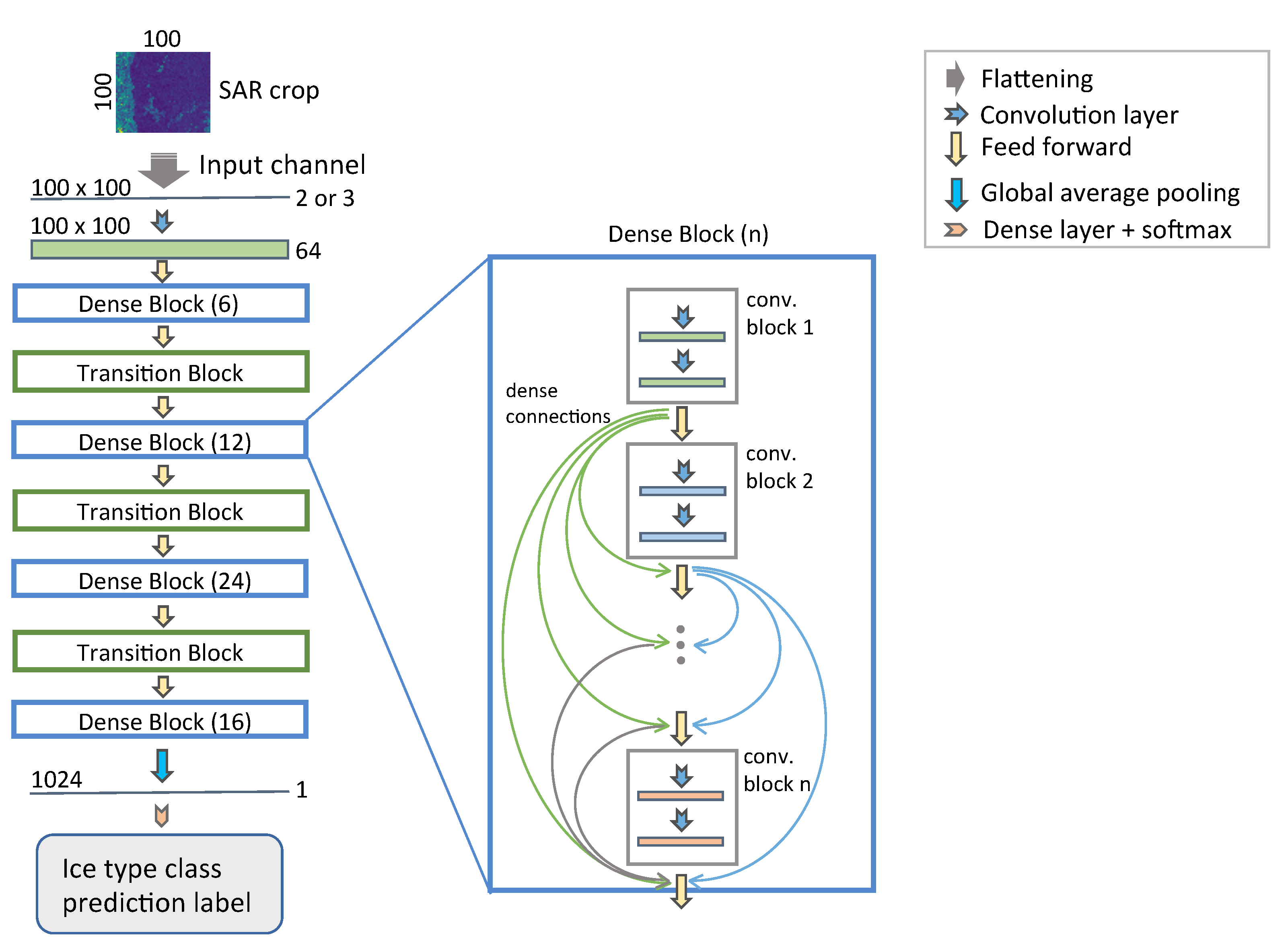
Although sea ice classification by type is the topic of this paper, it is important to review previous research that has been conducted on sea ice concentration estimation using deep learning to gain insights into other methodologies used to estimate ice characteristics. A recent study used a neural network called DenseNet [13] to estimate sea ice concentration from training on a dataset of 24 SAR images [14]. The authors of this paper used the ARTIST Sea Ice (ASI) algorithm [15] to label their dataset. This study experimented with a variety of factors and found that the accuracy of the model was dependent on the size of the patches used from the SAR images. The authors addressed over-fitting using data augmentation to increase the dataset size by adding varying degrees of Gaussian noise. The authors also developed a novel two-step training technique that consisted of first training a model with augmented data until convergence to a local minimum. Subsequently, a new model was initialized with the weights from the previous model and trained with a smaller learning rate on the dataset without augmentation. The authors hypothesized that noise injection into the SAR patches removed the relevance of texture information and led to degraded results. This training process was found to improve the results because the texture information relevance was recovered. However, there were difficulties predicting ice concentrations for thin new ice. Another study [16] used a five layer convolutional neural network to estimate sea ice concentration from SAR imagery. The dataset used in this study consisted of 11 HH and HV SAR images that were sub-sampled and labelled using CIS charts by extracting 41 × 41 sub-regions centred about the image analysis sample location denoted by latitude and longitude. The study found that the number of water samples contained in their dataset was about eight times greater than the next most common ice concentration class. Several approaches exist to work around such a disparity in the distribution of classes such as undersampling the majority, oversampling the minority, or using a Bayesian cross-entropy cost function, but the authors chose to train with the skewed dataset for a larger number of epochs (500) to get out of a local minimum found at early epochs due to the over representation of water.

The challenge in developing a deep learning classifier for sea ice type is the availability of a large number of accurately labelled data. Previous studies classifying ice types with neural networks labelled their datasets in a variety of ways. A pulse-coupled neural network (PCNN) was used with RADARSAT-1 ScanSAR Wide mode images over the Baltic Sea [17]. Therein, classes for supervised training were created by decomposing homogeneous regions in the SAR image into a mixture of Gaussian distributions using an expectation-maximization algorithm. These generated classes were then paired with the associated region in the SAR image and given to the PCNN for training. [18] generated classes for their dataset per the World Meteorological Organization (WMO) terminology [6]. Their dataset consisted of SAR patches along the path of an icebreaker, and the generated classes were based on in situ observations and other sensor information.

As an alternative to the labelling methods above, herein we assess the ability for a neural network to predict ice type from SAR data labelled using the stage of development feature from CIS ice charts. The labelling method is similar to the 2016 study done by Wang et al. [16], but is applied to the estimation of ice type, as opposed to ice concentration. While ice concentration is an important factor for naval navigation in the Arctic, our goal in this work is to predict ice stage of development. Knowledge of current ice type conditions can aid in the decision making process during naval routing because ships can break through regions where the ice concentration may be high, but the ice type is thin. Conversely, it is also important to know where the ice type is thick in order to avoid those regions.

In this paper, we present new algorithms for predicting sea ice stage of development based on a deep learning concept. We develop a methodology, in which we create labelled datasets using a combination of SAR images and CIS ice charts. A comparative analysis of the predictive performance of two different neural networks is completed. We conclude with an interpretation of our results and suggestions for the next stage of algorithm development.

2. Materials and Methods

2.1. Study Region

The Hudson Bay (the Bay) region seen in Figure 1a of the Canadian Arctic is important for shipping and other maritime activities [19]. Hudson Bay (coupled with James Bay) is the largest inland sea in North America at over 1,300,000 km² [20], with Arctic water entering through Roes Welcome Sound and Atlantic water entering through channels connecting Hudson Strait. Winters are characterized by seasonally varying ice cover between October and August, and the Bay generally exhibits colder temperatures than those at similar latitudes due to ice lasting into the late summer [20]. During summer, the Bay exhibits temperatures that are 5 to 10 °C cooler than the surrounding land, while during the winter, sea ice cover coupled with cooling Arctic Oscillation flow effects can result in temperatures reaching −45 to −50 °C Seasonal snowfall generally occurs in October and November, with totals reaching 120 to 150 cm in the northern part of the Bay. Due to the seasonal melt regime, the Bay contains first-year ice (FYI) [21] with a high concentration (10/10 coverage) and typical ice thickness reaching a maximum of ∼2 m (excluding rafting and ridging) with an average ice thickness of ∼1.6 m peaking in April and May [20].

Recent studies have shown that freeze-up is occurring later in the year and melt is occurring earlier in the year [21], and contemporary studies continue to investigate the linkage between field based observations and satellite measurements [22] during these critical times in the seasonal evolution. Although the inter-annual variability of sea ice extent is constrained by the surrounding land mass, ice extent in Hudson Bay decreased between 1978 and 1996 at a rate of 1400 km²/yr. [23]. Beginning in late May or early June, coastal leads (potentially navigable open water between shore and the remaining contiguous ice-pack) extend and broaden, encircling the Bay, with complete melt occurring during the following 4 to 5 weeks [20].

2.2. Description of Data Products

To create a dataset appropriate for deep learning classification of ice types, we consider 350 RADARSAT-2 (R2) ScanSAR Wide (SCW) images and 172 image analysis charts, herein referred to as Batch 4. The chosen dataset spans from June to December 2018 to obtain a distribution of labelled data representing the melt and freezing periods. The SCW images have a swath width of 500 km with a nominal pixel spacing of 50 m × 50 m and range between 20 degrees for the near incidence angle and 49 degrees for the far incidence angle [24]. The CIS sea ice charts serve as expert approximations to in situ conditions and are produced by ice analysts using R2 SAR imagery, as it is the main satellite data source for routine monitoring of the Canadian Arctic. The CIS ice analysts manually identify a set of spatial polygons for a given R2 SAR image, summarize the attributes of each polygon in the form of an egg code [25], and publish these results in image analysis charts. Examples of attributes in the egg are the total and partial ice concentrations, the stage of development (or ice type), and the predominant floe size range (or the form) of the ice. The CIS produces various types of satellite based ice charts, including image analysis charts and daily charts. We use image analysis charts as they correspond most closely to specific SAR images. An example SCW image is shown in Figure 1b.

2.3. Dataset Labelling

Image analysis ice charts are parsed to extract the stage of development feature (interchangeably referred to as ice type) from the egg codes in the CIS image analysis ice charts to provide labels for each SAR image in Batch 4. For the purposes of this study, egg codes having only a total sea ice concentration (Ct) ≥9+ are used. The egg codes are then simplified into a smaller set of ice type categories per

Table 1. Simplified labelling scheme reducing CIS egg codes to three classes.

Category	Label
Ice-free	0
New ice corresponds to the stage of development codes 1–5	1
First-year ice corresponds to the stage of development codes 6–4•	2

. The result of categorizing the eggs in this way is shown in Figure 1c.

Labels 1 and 2 for ice types encapsulate the stage of development codes consistent with Table 3.1 in the CIS manual, while label 0 for water is consistent with the ice-free diagram shown in Figure 2.2 in the CIS manual [25]. Old ice was not included in this study because it is not an ice type typically found in the Hudson Bay. This labelling scheme is referred to as Label Type 4 in the remainder of the paper to follow the historical development of the software framework used to conduct this study. This means three different labelling schemes were evaluated prior to Label Type 4 and were not suitable for the results presented in this paper. Furthermore, egg code samples are included in the dataset only if all sub-categories of the stage of development (Sa, Sb, Sc) map to the same label, which we refer to as pure samples, otherwise the sample is discarded. For example, suppose that Sa is given a code of 6 and Sb is given a code of 1 in the egg code produced by the CIS. Sa would map to a label of 2 and Sb would map to a label of 1 per Label Type 4 defined in Table 1. Since the sub-categories of the stage of development do not map to the same label in this example, the egg code is not included in the dataset.

2.4. SAR Sub-Region Extraction

The chosen labels are paired with sub-regions in the corresponding SAR image based on the latitude and longitude given in the image analysis ice chart. Each sub-region is chosen to be 100 × 100 pixels centred about the latitude and longitude coordinate of the egg code. A 100 × 100 pixel sub-region is chosen to be consistent with the ice charts that are rasterized by the CIS experts with a 5 km × 5 km pixel resolution, wherein the pixel size of a SAR image represents a 50 m × 50 m area. The R2 products use a rigorous projection model to describe the mapping between image coordinates $(x,y)$ and ground coordinates $(lat,lon,height)$ [26]. The approximation used for the rigorous projection model is given by a set of rational polynomials, and normalized polynomial coefficients are given in the Product Information File (PIF) of the R2 SAR product. The image coordinates of the centre of each sub-region in a SAR image for the given latitude and longitude associated with an egg code are calculated using the coefficients and the rational polynomials detailed in [27]. Example sub-regions for one of the SAR images used in the dataset are shown in Figure 2.

Note that the sub-regions shown in Figure 2 do not appear to be square because the WGS84 projection causes warping of the SAR image and the sub-regions. The correctness of the sub-regions can be verified by measuring the length of the edges of the sub-regions in a GIS application. The same sub-regions in both HH and HV polarizations of SCW images are used to form the first two channels of an input sample to be used in the machine learning classification. The cross-polarization (cross-pol) ratio of HV/HH is appended to the sample as a third channel to provide additional information as the ratio is sensitive to volume scattering within a medium. The input sample is therefore a 3D object with a shape of (3, 100, 100), and each is labelled per Table 1. Once labelled, the sub-region and the label are treated as an independent sample. We acknowledge that calibration and noise removal information is provided with the SAR products and can be used to pre-process the images, but for this proof of concept, we sought a streamlined framework that could be used in an operational capacity for sea ice service entities while still providing accurate results.

2.5. Model Setup

Two different convolutional neural networks (CNN) are used for training. The first neural network is modelled after the encoder section of U-Net [28] and is shown in Figure 3. Sea ice classification is naturally an image segmentation problem, and U-Net has been shown to be effective for this particular type of application, as in [29], which applied a U-Net based architecture on the Cityscapes dataset, and in [30], which applied U-Net to segment surface ice concentration on images of two Alberta rivers. Only the encoder section is used because the methodology chosen to create our dataset assigns class labels that are single-valued. The encoder section of U-Net consists of four convolution blocks, where each block is formed by two convolution layers followed by a max-pooling layer. The number of convolution filters after each convolution block doubles.

The second CNN used for training is DenseNet [13]. DenseNet was chosen as it has been shown to achieve state-of-the-art results on challenging datasets such as ImageNet [13]; it was also used in a previous study to estimate sea ice concentration with promising results [14]. A general block diagram of the DenseNet used in this work is shown in Figure 4. One of DenseNet’s properties is its capability to reuse features at different scales throughout the network, which applies nicely to SAR images where important features are recurrent at different scales. Feature reuse is achieved within the dense blocks shown in Figure 4. A dense block is composed of a series of convolution blocks whose output is concatenated with the input of every subsequent convolution block via skip connections. DenseNet’s authors showed that output concatenation (as opposed to output summation found in residual networks) enables the model to more efficiently reuse features [13]. The DenseNet model consists of a series of these dense blocks and transition blocks, the latter of which consist of a bottlenecking convolution layer and an average pooling layer.

The DenseNet configuration used in this study is DenseNet-121, indicating that there are 121 layers in the model. This is achieved by having four dense blocks, each having 6, 12, 24, and 16 convolution blocks, respectively, where each convolution block consists of 2 convolution layers, contributing 116 layers. One transition layer is used between each dense block, thereby adding another 3 layers to the total. The two remaining layers come from an initial convolution layer and the classification layer. Note that the initial convolution layer is typically used to down-sample larger inputs, but is not necessary for our 100 × 100 pixel input.

Both the U-Net based and DenseNet models use softmax as the classification layer to assign an ice type class probability to a given input. The softmax probabilities are given by Equation (1),

$$p(y^{(n)}=k|{\mathbf{x}}^{(n)};\mathbf{W})=\frac{e^{{\mathbf{w}}_k^T{\mathbf{x}}^{(n)}}}{{\sum }_{k^{\prime }=1}^K{e}^{{\mathbf{w}}_{k^{\prime }}^T{\mathbf{x}}^{(n)}}}$$

(1)

where $y^{(n)}$ is the output class label for the nth sample, ${\mathbf{x}}^{(n)}$ are the outputs of the last layer, and ${\mathbf{W}}^T=[{\mathbf{w}}_1{\mathbf{w}}_2\dots {\mathbf{w}}_K]$ are the weights of the last layer. These probabilities are optimized through a categorical cross-entropy loss function L given by Equation (2), where ${\delta }_{nk}$ is the Kronecker delta.

$$L=-\sum _{n=1}^N\sum _{k=1}^K{\delta }_{nk}log(p(y^{(n)}=k|{\mathbf{x}}^{(n)};\mathbf{W}))$$

(2)

2.6. Training Setup

The dataset created per the methodology in this section generated 186,673 water samples, 14,539 new ice samples, and 63,265 first-year ice samples. The dataset was balanced such that the loss is not over- or under-represented for any particular class during training [31], and this was accomplished by undersampling the majority and randomly keeping 14,539 samples in each class. These samples were randomly shuffled and split into an 80%-10%-10% training, validation, and testing set. These subsets were z-score normalized by first calculating the mean and standard deviation of each channel across all training samples. This set the mean and variance of the subsets to 0 and 1, respectively, to provide better gradient flow during training. The gradients were calculated with backpropagation, and the weights were updated with the Adam optimizer. Additionally, training was conducted in batch sizes of 1000 for the adapted model of U-Net and 32 for DenseNet; the DenseNet model had smaller batch sizes due to GPU memory constraints and the increasingly large array sizes arising from concatenation in the model. Methods for improving memory efficiencies in DenseNet models using a different deep learning framework can be found in the literature [32], but are not considered here.

3. Results

In order to prove the concept of using CIS labels and deep learning to predict ice type, several experiments were conducted by changing the dataset in a variety of ways. The performances of the U-Net based model and DenseNet model were simply quantified using the percentage of correctly classified samples. We refer to this metric as the accuracy. Additional insight was obtained by a second metric aligned with the goal of this proof of concept to predict ice types. We define the ice accuracy metric as the sum of the true positive samples for Ice Classes 1 and 2 based on Table 1 divided by the total number of samples in those ice classes. The ice accuracy was formulated to better compare experiments with unbalanced datasets since certain experiments had a large number of water samples compared to ice samples (greater than a 7:1 ratio before undersampling the majority). The best experiment achieved an overall accuracy of 94.02% and an ice accuracy of 91.75% on the test set.

3.1. Experimental Configurations

The software framework developed for this work was created to flexibly support the six configurable parameters that were used to uniquely identify different experimental datasets. These parameters are described and itemized below and their values are summarized in

Table 2. Dataset configuration naming map.

	1	2	3	4	5	6
	Data Batch	DEX Type	Label Type	Polarizations	Total Concentration	Pre-Processing
A	-	-	-	-	-	Raw
B	-	DEXI	-	-	-	-
C	-	-	-	-	Ct≥ 9+	-
D	Batch 4	-	Label Type 4	HH, HV	-	-
E	-	-	Label Type 5	-	-	-
F	-	-	-	-	-	-
G	-	-	-	HH, HV, HV/HH	-	-

.

• Data batch—indicates the SAR scenes and CIS data source files to use. In this work, only Batch 4 is considered, whereas previous iterations of data batches consisted of different subsets of source files leading up to Batch 4.
• DEX type—determines the type of CIS data to use, DEXA being a code for daily ice charts and DEXI being a code for image analysis charts. In this work, only DEXI is used.
• Label type—specifies the egg code labelling type used. Only Label Types 4 and 5 are used in this work. Label Type 4 refers to the set of labels defined in Table 1. Label Type 5 modifies the labels in Table 1 to group new ice (label 1) and first-year ice (label 2) into a single class, producing a two class experiment used to benchmark the Label Type 4 experiments.
• Polarization—specifies the SAR polarizations included as input channels in the dataset. Only two channel input samples with HH and HV polarizations and three channel input samples with HH, HV, and the HV/HH ratio are used in this study.
• Total concentration (Ct)—indicates the minimum Ct required from the egg code for a sample to be included in the dataset. Only samples with concentrations ≥ 9+ were considered in this study.
• Pre-processing—determines the pre-processing steps to use on the SAR samples. No pre-processing was considered in this study.

For example, the experimental configuration DBDDCA decodes to the configuration parameter values: Batch 4 (D), DEXI charts (B), Label Type 4 (D), HH and HV polarization channels (D), ice concentration ≥9+ (C), and no pre-processing (A). For the purposes of this study, the parameters for data batch, DEX type, total ice concentration, and pre-processing (i.e., the first two and last two letters in the dataset identification code) can be ignored by the reader. Only the label type, which denotes two and three class experiments, and the polarization parameters were varied (i.e., the middle two letters of the dataset identification code). Unpopulated entries in the table refer to parameter values not used in this study, but are maintained for historical and future continuity.

3.2. Experimental Results—Summary and Interpretation

The resulting accuracy metrics of the U-Net based model and the DenseNet model are summarized in

Table 3. U-Net based classifier results.

			Training			Testing
Config.	# Classes	# Channels	Loss	Acc. %	Ice Acc. %	Loss	Acc. %	Ice Acc. %
DBEDCA 1	2	2	0.0190	99.37	99.32	0.0337	99.05	98.99
DBEGCA 1	2	3	0.0128	99.59	99.45	0.0356	99.01	98.90
DBDDCA	3	2	0.1378	94.76	92.62	0.1742	92.99	90.51
DBDGCA	3	3	0.0741	97.49	96.51	0.2371	91.75	88.48

¹ Two class classifier benchmark experiments.

and

Table 4. DenseNet based classifier results.

			Training			Testing
Config.	# Classes	# Channels	Loss	Acc. %	Ice Acc. %	Loss	Acc. %	Ice Acc. %
DBEDCA 1	2	2	0.0244	99.37	99.13	0.0329	99.07	98.65
DBEGCA 1	2	3	0.0225	99.42	99.17	0.0309	99.10	98.65
DBDDCA	3	2	0.1414	95.95	94.23	0.1872	94.02	91.75
DBDGCA	3	3	0.1129	97.21	96.02	0.2008	93.12	90.34

¹ Two class classifier benchmark experiments.

, respectively. The experiments that were performed for the purposes of this proof of concept sought to compare the performance of training on datasets with two channel inputs (HH, HV) and three channel inputs (HH, HV, HV/HH). The experiments conducted for the three class dataset (Label Type 4 with water, new ice, and first-year ice classes) were also replicated with the corresponding two class dataset (Label Type 5 with water and ice classes) for benchmarking purposes.

There are a few patterns that emerged based on the experimental results shown in these tables. The first is that, as expected, none of the three class classifiers were able to achieve the same level of accuracy as the two class classifiers. The obvious explanation for this difference is that samples of two different ice types are more difficult to distinguish than water and ice. Another possibility for the discrepancy is the number of samples with which the models were trained. The two class experiments had 81,928 samples for each class, while the three class experiments had only 14,539 samples. The choice to balance the datasets by undersampling the majority contributed the most to this difference. The effects of undersampling the majority on the number of samples in each class are outlined in

Table 5. Effects of under-sampling the majority demonstrating the differences between the full dataset and balanced samples.

	Before			After
Label Type	Class 0	Class 1	Class 2	Class 0	Class 1	Class 2
2 Class	186,673	81,928	-	81,928	81,928	-
3 Class	186,673	14,539	58,726	14,539	14,539	14,539

. Undersampling the majority in the three class case can be seen to have eliminated 172,134 samples of water and 58,726 samples of first-year ice, compared to the two class case that only eliminated 104,745 water samples. The other factor that caused such a large difference in the number of samples available between the two and three class datasets was the choice to reject impure egg code samples whose sub-categories of the stage of development feature did not all map to the same ice type. Rejected impure samples in the three class case accounted for a relative increase of 4124 pure samples in the two class case, widening the gap even further. This occurred because the sub-categories for the stage of development feature (Sa, Sb, Sc) mapped to the same label in the two class case (resulting in pure samples), but mapped to different labels in the three class case (resulting in rejected impure samples).

The second pattern to notice from the accuracy results is that DenseNet consistently outperformed the U-Net based model. This was not a surprising result since the U-Net based model was adapted to fit the needs of the dataset formulation, while the DenseNet architecture is more naturally suited to the problem. The modified U-Net architecture only has 1.2 million trainable parameters compared to DenseNet’s seven million, which allows DenseNet to have more representational power over the modified U-Net, which could explain the differences in the results. The size of DenseNet came at the cost of a 6.58 h training time (for the DBDDCA experiment with two polarization channels and three classes), compared to the 19 min required to train the U-Net based model for the same experiment. DenseNet is also a memory-hungry model, and even with a modern GPU (16 GB Tesla V100 GPU), only batch sizes of 32 could be used to train this model compared to the batch size of 1000 used to train the U-Net based model. According to the creators of DenseNet, improvements can be made to improve memory efficiency, but their implementation was not immediately compatible with the deep learning framework used to conduct these experiments [32]. We will investigate memory improvements in future work. While the differences in batch size clearly impact the training time, it is unclear if they affect performance. A recent study showed that models trained with smaller batch sizes achieve better testing results than models trained with larger batch sizes [33]. Training the U-Net model with the same batch size of 32 would clarify whether or not this was the cause for the discrepancy in the results. Nonetheless, an approximate 1% difference in accuracy is not a bad trade-off to be made for a fraction of the training time required.

The third pattern is that experiments that used three polarizations channels (HH, HV, HV/HH) in the input sample performed markedly better than the two channel experiments (HH, HV) on the training set, but performed slightly worse on the test set. A possible explanation for this behaviour is that the HV/HH ratio channel is not independent of the HV and HH channels and that supplying this additional information alleviates the model from learning that the ratio between the two channels could provide beneficial features. As a consequence, the model could overfit the training set, degrading the model’s ability to generalize to the unseen test data. Further experimentation in the form of model regularization is needed to assess whether or not overfitting is occurring and will be the subject of a future study.

3.3. Experimental Conclusions

While the analysis of the differences between numerical results was necessary to gain insights into the possible variables that caused them, a visual representation of the predictions can serve as a reminder that the goal of this work is to provide a proof of concept that this methodology could be sufficient to automate classification of ice types prior to the analysis of a sea ice expert. Three SAR scenes were selected to showcase the predictive quality of the experiment that achieved the highest test set results, which was a DenseNet model trained on the DBDDCA (three classes, two channels) experiment dataset. Figure 5 shows samples extracted from the SAR images that were dedicated to the training set and the testing set, as well as the corresponding predictions made from each sample. The plots in Figure 5 show that some of the erroneous predictions may be identified by an ice analyst based on the proximity to other samples.

The capacity of a neural network to accurately predict ice types during the summer melt season was the other research question to be answered by this proof of concept. A monthly breakdown of the samples in the training and testing set and their class for the DBDDCA experiment is given in

Table 6. DenseNet DBDDCA (3 class, 2 channel) monthly count breakdown.

	Training				Testing
Month	Class 0	Class 1	Class 2	% of Total	Class 0	Class 1	Class 2	% of Total
Jun.	0	0	11,600	33.24	0	0	1435	32.89
Oct.	5017	489	0	15.78	644	64	0	16.23
Nov.	6606	3946	0	30.24	811	474	0	29.45
Dec.	0	7177	58	20.73	0	932	3	21.43
Total	11,623	11,612	11,658	100.00	1455	1470	1438	100.00

and

Table 7. DenseNet DBDDCA (3 class, 2 channel) monthly accuracy breakdown.

	Training				Testing
Month	Class 0	Class 1	Class 2	Acc. %	Class 0	Class 1	Class 2	Acc. %
Jun.	-	-	95.54	95.54	-	-	92.96	92.96
Oct.	98.70	87.12	-	97.68	97.20	79.69	-	95.62
Nov.	99.89	93.84	-	97.63	99.63	90.72	-	96.34
Dec.	-	93.44	17.24	92.83	-	91.52	0.00	91.23
Total	99.38	93.31	95.15	97.95	98.56	90.75	92.77	94.02

.

It can be seen from this analysis that classes 0 and 1 were not represented during the month of June, which was during the summer melt season. This was due to the sampling restrictions of using “ice-free” only image analysis labels to represent Class 0 and choosing to only use egg codes with ice concentrations ≥9+ to represent Classes 1 and 2. Rationally, the ice concentration should decrease during the summer melt season as ice breaks up and a given area is occupied by more water. While this limits the conclusions that can be made about summer melt accuracy, it can be seen that all three classes had a testing accuracy over 90%, where the new ice class was the lowest at 90.75%. This suggests that the neural network had more difficulty recognizing features that can distinguish between ice types than it did in distinguishing between water and ice, and this was consistent with the analysis in Section 3.2 that compared results between the two class and three class experiments. This conclusion is also supported by the confusion matrices for the training and test sets shown in

Table 8. DenseNet DBDDCA (3 class, 2 channel) confusion matrices.

		True Condition
		Training			Testing
		Class 0	Class 1	Class 2	Class 0	Class 1	Class 2
Prediction Condition	Class 0	11551	30	76	1434	5	17
	Class 1	8	10835	489	2	1334	87
	Class 2	64	747	11,093	19	131	1334

.

It is clear that the neural network misclassified ice samples as other ice classes more than it misclassified them as water. As for the outliers of 17.24% and 0% for the training and testing accuracies that can be seen for Class 2 in the month of December in Table 7, these cases consisted of 58 and three samples, respectively, which was too small of a sample size for any conclusion to be made. Generally speaking however, the 91.75% ice accuracy achieved by DenseNet showed that neural networks can be used to effectively classify between new and first-year ice.

4. Discussion

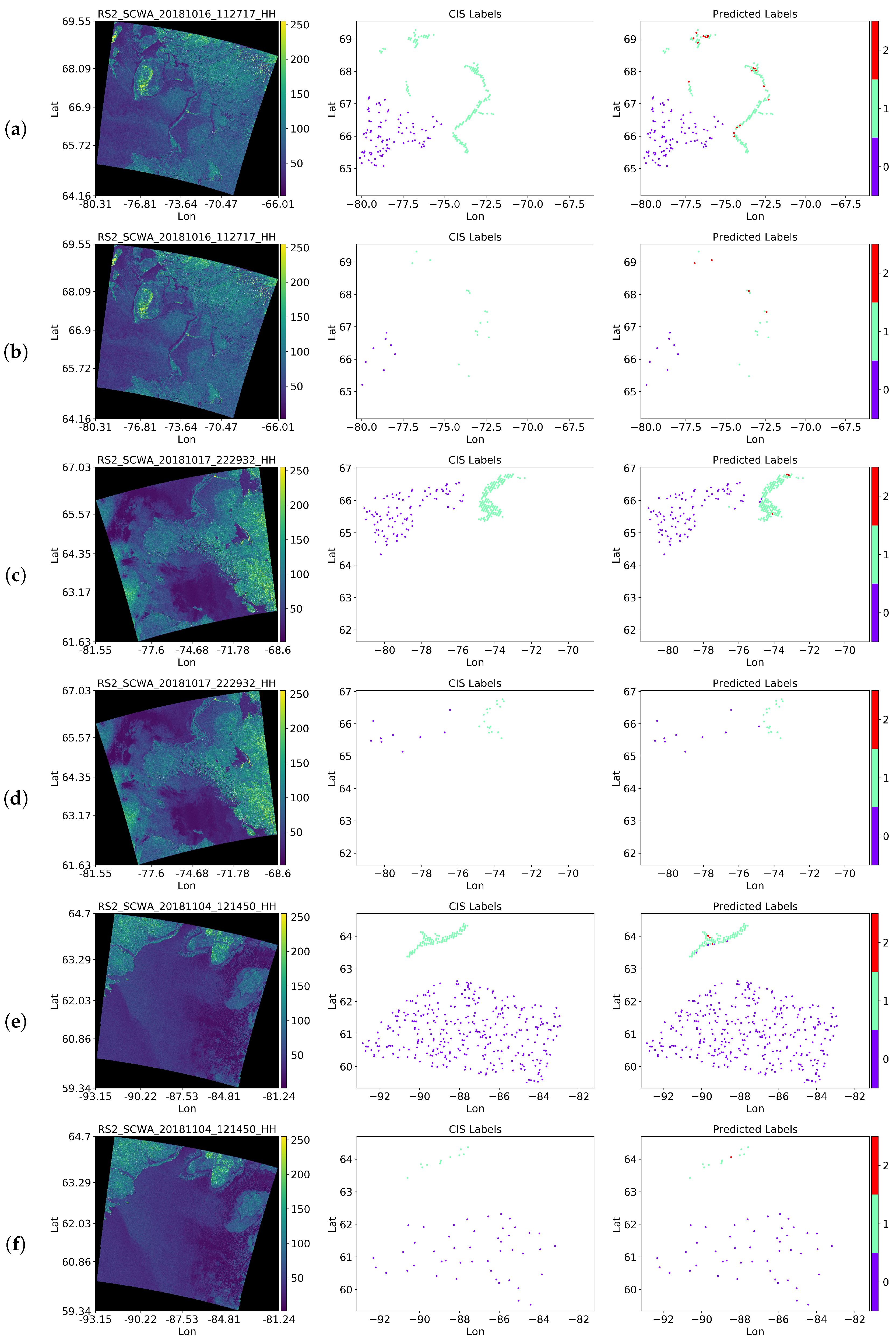
We showed that DenseNet accurately learns from expertly labelled data to classify between water and ice for the two class case, as well as water, new ice, and first-year ice for the three class case, using only uncalibrated HH and HV SAR images. The two class classifier provides a good baseline for the three class classifier as it sets upper-limit performance expectations. DenseNet consistently outperformed the U-Net based model, and it was observed that three channels in the input sample performed better than two channel experiments on the training set, but performed slightly worse on the test set. The visual representation of the predictions demonstrated that erroneous predictions could be rectified by sea ice experts based on the bulk of correctly classified samples that are in proximity to the erroneous predictions. An analysis of the class accuracy showed that the neural network would have a greater chance of producing erroneous predictions between ice types than it would between water and ice. No conclusions could be made concerning the accuracy of the model during the summer melt season due to the lack of representational data. Sea ice classification during the summer melt period has been attempted by others with little success. Our inability to assess the predictive quality of sea ice classification during the summer melt season using the tested neural networks herein was primarily due to the lack of representational data of all three classes during the month of June.

With the goal of producing accurate, high-resolution maps of Arctic marine conditions for industrial and marine transportation, it is also important to compare the results found in this study with existing systems and results from other published work, beyond the two class experiments that were conducted here to benchmark our own result. The study completed by [17] generated six distributions using the expectation-maximization algorithm, which were used to label their dataset for training. While [17] used a different labelling scheme than the one presented in this paper, a relatively similar behaviour was observed. The PCNN model used in their study to segment ice types also misclassified ice with other ice types, fast ice in particular. Unfortunately, no metrics were provided by the authors to assess the classification accuracy; therefore, no further comparison can be made with our results. The study completed by [18] used the WMO terminology to label their dataset into six classes based on in situ observation. The six classes were smooth, medium, deformed first-year ice, young ice, nilas, and open water. The total accuracy achieved among these six classes was 91.2% with a neural network using a fusion of three types of data (ERS, RADARSAT SAR, and Meteor Visible) and noted that the addition of images in the visible spectrum helped improve classification between nilas and open water. While our results cannot be compared directly, due to the differences in the labelling methods and number of classes, the results found in [18] showed similar levels of accuracy.

With limited available studies using deep learning and CIS labelled data for comparison of ice type classification, here we conduct comparisons with similar work for sea ice concentration. The study presented in [14] used a DenseNet model to predict sea ice concentration from SAR imagery. The training labels used in that study were obtained from passive microwave data and determined by the ASI algorithm; the results were also compared to CIS charts. While this does not directly compare to the results presented herein, the error metrics used to evaluate performance achieved a similar error rate. Specifically, the test set error in [14] was 7.87%, while the overall error found in our results was 5.98%. This shows that DenseNet can be used effectively to achieve good results in two different applications relating to the same input data with different outputs, a testament to the flexibility and generalizability of the deep learning model. Similarly, the study presented in [16] also used a convolutional neural network (though not the same as DenseNet or U-Net) to predict sea ice concentration from SAR imagery. Therein, the methodology used to generate and label the dataset was similar to the methodology presented here, the only difference being in the resulting output. Given that estimating sea ice concentration is a regression problem, the L1 mean error metric was used in [16] to report a 0.08 average $E_{L1}$ score. While this metric is not comparable to classification accuracy, the low error score achieved supports accurate prediction of ice characteristics with deep neural networks using SAR imagery, which is a similar experimental finding of the work herein.

4.1. The Utility of DenseNet for Sea Ice Mapping

The methodology presented in this paper can be applied towards the mapping of sea ice type in the Arctic by following a few steps. An incoming SAR image would be uniformly subdivided into 100 × 100 sub-regions without overlap as a first step. The collection of sub-regions would then be filtered such that sub-regions containing known land masses are removed from the collection. For accuracy purposes, it may also be desirable to exclude sub-regions having <80% of their pixels represent valid SAR data in order to imitate the samples used in the training set. The remaining sub-regions would then be processed and classified by the trained DenseNet model from this study into water, new ice, or first-year ice and assembled to form a segmented image. The time required for DenseNet to completely label a typical 10,000 × 10,000 pixel SAR image that has been pre-subdivided was approximately 40 s on a modern high-end GPU. This shows that DenseNet can automate the prediction of sea ice by type from SAR images to generate image analysis ice charts in a timely manner.

4.2. Future Work

The presented three class models for predicting CIS ice types from SAR imagery can be easily extended within the scope of the configurable parameters used to identify different datasets. As a first step to furthering the research to make it useful to operational sea ice services, the labelling type must be expanded to increase the number of ice classes. There are a total of 14 classes that CIS ice experts use to classify ice based on its stage of development [25]. Given the success that both neural networks used in this study achieved on the experiments conducted, in particular the three class experiments, a natural next step would be to assess the performance of these neural networks in a similar manner for incremental class definitions from three to 14 class setups. In doing so, we should also study the relaxation of the ice concentration criteria to include more egg codes in order to increase the chances of obtaining a sufficient number of samples for each of the 14 classes, even though such an action would come at the cost of having impure samples in the sense that they will be a mix of water and ice. In addition to reducing purity requirements, class samples for each of the 14 ice classes can also be increased by expanding the region of interest and time of year. By expanding space and time, we will also be able to better assess the ability for the proposed networks to accurately classify ice type during seasonal melt and fall freeze-up.

We expect that as supported ice type classes are expanded, improvements to the dataset and model can be made to improve classification performance. Staying within the scope of the configurable parameters used to identify datasets, further testing should be conducted to assess the effects of calibration and noise removal on the accuracy of ice classification. This can be accomplished by using additional information provided with the SAR products detailing corrective gain values and noise signals [26]. Furthermore, including a third channel for the HV/HH polarization ratio improved the three class classification accuracy between ice types, at least on the training set. Therefore, future work should also include the effects of regularization techniques on the models, in an attempt to translate the improved training set performance to unseen data.

To strengthen the case that this proof of concept is a viable method to classify ice by type, future studies with more ice types should include K-cross-validation for each experiment to verify the predictive quality and generalizability of the models. The difference in accuracy between each experiment in this proof of concept was within the range caused by random initialization of the models. K-cross-validation would also reduce the uncertainty that the differences in accuracies are caused by random initialization.

Another avenue for future research goes outside the confines of the current framework by constructing a dataset better suited for the complete encoder-decoder U-Net architecture. Although the results for the three class experiments conducted were good, the models treated each sample sub-region as an independent sample. However, sub-regions that are close in proximity to each other will be logically dependent on one another, with similarities in ice conditions. This is where the U-Net architecture would be able to extract the spatial context of nearby samples to hopefully provide better segmentation results. U-Net was designed with this aspect in mind and uses skip connections between the encoder and decoder in order to localize and contextualize features from the macro-resolution of the encoder with the generated micro-resolution features from the decoder side. U-Net also generates feature maps at various scales with different contexts, which is important for SAR imagery as features at large scales tend to appear at finer resolutions as well.

While this is a lengthy list of extensions that can be made to this work, they were not applied; however, the proof of concept was sufficiently validated to show that there is merit in pursuing these changes/improvements for broader ice type classification.

5. Conclusions

This study consisted of a proof of concept that neural networks could be used to classify ice types effectively using SAR imagery and CIS image analysis ice charts as labelled data. The SAR images were cropped into sub-regions per the latitude and longitude coordinates given for each ice sample egg code in the CIS image analysis ice chart, and each sub-region was treated as an independent sample. Experiments were conducted on datasets that had input samples consisting of a fusion of both HH and HV polarizations for each sub-region, and other experiments also added a third channel using the ratio of HV/HH. These datasets were labelled based on a simplification of the egg code samples from the CIS image analysis ice charts in two ways. The first labelling type was a simple water and ice categorization, which was used to benchmark experiments of the second labelling type, which consisted of three categories that described water, new ice, and first-year ice. Two neural networks were trained on these datasets, one of which was a modified U-Net architecture, and the other was a DenseNet. The DenseNet architecture achieved the highest overall accuracy of 94.02% and the highest ice accuracy of 91.75% on the three class dataset with the dual-pol HH and HV configuration. An analysis of the prediction results produced by DenseNet showed that the neural network experienced some more difficulty distinguishing between ice samples of different types than it did distinguishing between water and ice samples; however, the majority (>90%) of ice samples were still correctly classified. The lack of representative data for the three classes for the months of June, October, November, and December, important to seasonal classification of sea ice melt and formation, resulted in an inability to draw conclusions about the performance of the model with respect to seasonality. To resolve this issue, further experimentation is necessary to test if the classification of ice type in the summer and fall season can be established through a relaxation of the ice concentration criteria by including impure samples (in the sense that they will be a mix of water and ice). The results presented in this work validate the proof of concept that a neural network can be used to effectively automate the pre-categorization of different ice types based on SAR imagery and segment a typical 10,000 × 10,000 SAR image in a timely manner for further expert analysis.

References

1. Komarov, A.S.; Caya, A.; Buehner, M.; Pogson, L. Assimilation of SAR Ice and Open Water Retrievals in Environment and Climate Change Canada Regional Ice-Ocean Prediction System. IEEE Trans. Geosci. Remote Sens. 2020, 58, 4290–4303. [Google Scholar] [CrossRef]
2. Carter, N.A.; Dawson, J.; Joyce, J.; Ogilvie, A. Arctic Corridors and Northern Voices: Governing Marine Transportation in the Canadian Arctic (Arviat, Nunavut Community Report). Available online: https://ruor.uottawa.ca/handle/10393/36924 (accessed on 31 July 2020).
3. Barber, D.; Babb, D.; Ehn, J.; Chan, W.; Matthes, L.; Dalman, L.; Campbell, Y.; Harasyn, M.; Firoozy, N.; Theriault, N.; et al. Increasing mobility of high Arctic sea ice increases marine hazards off the east coast of Newfoundland. Geophys. Res. Lett. 2018, 45, 2370–2379. [Google Scholar] [CrossRef]
4. Ulaby, F.; Long, D. Microwave Radar and Radiometric Remote Sensing; Artech House: Norwood, MA, USA, 2015. [Google Scholar]
5. Barber, D.G. Microwave remote sensing, sea ice and Arctic climate. Phys. Can. 2005, 61, 105–111. [Google Scholar]
6. World Meteorological Organization. WMO Sea-Ice Nomenclature: Terminology, Codes, Illustrated Glossary and Symbols; Secretariat of the World Meteorological Organization: Geneva, Switzerland, 1970. [Google Scholar]
7. Howell, S.E.; Small, D.; Rohner, C.; Mahmud, M.S.; Yackel, J.J.; Brady, M. Estimating melt onset over Arctic sea ice from time series multi-sensor Sentinel-1 and RADARSAT-2 backscatter. Remote Sens. Environ. 2019, 229, 48–59. [Google Scholar] [CrossRef]
8. Yackel, J.J.; Gill, J.P.; Geldsetzer, T.; Fuller, M.C.; Nandan, V. Diurnal scale controls on C-band microwave backscatter from snow-covered first-year sea ice during the transition from late winter to early melt. IEEE Trans. Geosci. Remote Sens. 2017, 55, 3860–3874. [Google Scholar] [CrossRef]
9. Isleifson, D.; Hwang, B.; Barber, D.G.; Scharien, R.K.; Shafai, L. C-Band Polarimetric Backscattering Signatures of Newly Formed Sea Ice During Fall Freeze-Up. IEEE Trans. Geosci. Remote Sens. 2010, 48, 3256–3267. [Google Scholar] [CrossRef]
10. Soh, L.; Tsatsoulis, C. Unsupervised segmentation of ERS and radarsat sea ice images using multiresolution peak detection and aggregated population equalization. Int. J. Remote Sens. 1999, 20, 3087–3109. [Google Scholar] [CrossRef]
11. Scheuchl, B.; Cumming, I.; Hajnsek, I. Classification of fully polarimetric single- and dual-frequency SAR data of sea ice using the Wishart statistics. Can. J. Remote Sens. 2005, 31, 61–72. [Google Scholar] [CrossRef]
12. Kim, M.; Im, J.; Han, H.; Kim, J.; Lee, S.; Shin, M.; Kim, H.C. Landfast sea ice monitoring using multisensor fusion in the Antarctic. GISci. Remote Sens. 2015, 52, 239–256. [Google Scholar] [CrossRef]
13. Huang, G.; Liu, Z.; Maaten, L.V.D.; Weinberger, K.Q. Densely Connected Convolutional Networks. In Proceedings of the 2017 IEEE Conference on Computer Vision and Pattern Recognition (CVPR), Honolulu, HI, USA, 21–26 July 2017. [Google Scholar] [CrossRef] [Green Version]
14. Cooke, C.L.V.; Scott, K.A. Estimating Sea Ice Concentration From SAR: Training Convolutional Neural Networks With Passive Microwave Data. IEEE Trans. Geosci. Remote Sens. 2019, 57, 4735–4747. [Google Scholar] [CrossRef]
15. Spreen, G.; Kaleschke, L.; Heygster, G. Sea ice remote sensing using AMSR-E 89-GHz channels. J. Geophys. Res. Ocean. 2008, 113, C02S03. [Google Scholar] [CrossRef] [Green Version]
16. Wang, L.; Scott, K.A.; Xu, L.; Clausi, D.A. Sea Ice Concentration Estimation During Melt From Dual-Pol SAR Scenes Using Deep Convolutional Neural Networks: A Case Study. IEEE Trans. Geosci. Remote Sens. 2016, 54, 4524–4533. [Google Scholar] [CrossRef]
17. Karvonen, J.A. Baltic Sea ice SAR segmentation and classification using modified pulse-coupled neural networks. IEEE Trans. Geosci. Remote Sens. 2004, 42, 1566–1574. [Google Scholar] [CrossRef]
18. Bogdanov, A.V.; Sandven, S.; Johannessen, O.M.; Alexandrov, V.Y.; Bobylev, L.P. Multisensor approach to automated classification of sea ice image data. IEEE Trans. Geosci. Remote Sens. 2005, 43, 1648–1664. [Google Scholar] [CrossRef] [Green Version]
19. Andrews, J.; Babb, D.; Barber, D.G. Climate change and sea ice: Shipping accessibility on the marine transportation corridor through Hudson Bay and Hudson Strait (1980–2014). Elem. Sci. Anthr. 2017, 5, 15. [Google Scholar] [CrossRef] [Green Version]
20. Martini, I. Coastal features of Canadian inland seas. In Elsevier Oceanography Series; Elsevier: Amsterdam, The Netherlands, 1986; Volume 44, pp. 117–142. [Google Scholar]
21. Hochheim, K.P.; Barber, D.G. An update on the ice climatology of the Hudson Bay system. Arctic Antarct. Alp. Res. 2014, 46, 66–83. [Google Scholar] [CrossRef] [Green Version]
22. Harasyn, M.L.; Isleifson, D.; Chan, W.; Barber, D.G. Multi-scale observations of the co-evolution of sea ice thermophysical properties and microwave brightness temperatures during the summer melt period in Hudson Bay. Elem. Sci. Anthr. 2020, 8, 16. [Google Scholar] [CrossRef] [Green Version]
23. Parkinson, C.L.; Cavalieri, D.J.; Gloersen, P.; Zwally, H.J.; Comiso, J.C. Arctic sea ice extents, areas, and trends, 1978–1996. J. Geophys. Res. Ocean. 1999, 104, 20837–20856. [Google Scholar] [CrossRef]
24. Slade, B. RADARSAT-2 Product Description. RN-SP-52-1238 2018. Available online: https://mdacorporation.com/docs/default-source/technical-documents/geospatial-services/52-1238_rs2_product_description.pdf (accessed on 31 July 2020).
25. MANICE, CIS. Manual of Standard Procedures for Observing and Reporting Ice Conditions, 9th ed.; Canadian Ice Service (CIS), Meteorological Service of Canada: Ottawa, ON, Canada, 2005. [Google Scholar]
26. MacDonald, D. Ltd. Radarsat-2 Product Format Definition; RN-RP-51-2713; MDA Corporation: Richmond, BC, Canada, 2008; Available online: https://mdacorporation.com/docs/default-source/technical-documents/geospatial-services/radarsat-2-product-format-definition.pdf?sfvrsn=4 (accessed on 31 July 2020).
27. MacDonald, D. Ltd. Geolocation of RADARSAT-2 Georeferenced Products; Technical Report, Tech. Rep. RN-TN-53-0076; MDA Corporation: Richmond, BC, Canada, 2010; Available online: https://mdacorporation.com/geospatial/international/satellites/RADARSAT-2/docs/default-source/technical-documents/geospatial-services/rn-tn-53-0076-geolocation-tn-1-3.pdf?sfvrsn=4 (accessed on 31 July 2020).
28. Ronneberger, O.; Fischer, P.; Brox, T. U-Net: Convolutional Networks for Biomedical Image Segmentation. International Conference on Medical Image Computing and Computer-Assisted Intervention, Munich, Germany, 5–9 October 2015; Springer: Cham, Switzerland, 2015; pp. 234–241. [Google Scholar]
29. Siam, M.; Gamal, M.; Abdel-Razek, M.; Yogamani, S.; Jagersand, M. RTSeg: Real-time Semantic Segmentation Comparative Study. arXiv 2018, arXiv:cs.CV/1803.02758. [Google Scholar]
30. Singh, A.; Kalke, H.; Loewen, M.; Ray, N. River Ice Segmentation with Deep Learning. arXiv 2019, arXiv:cs.CV/1901.04412. [Google Scholar] [CrossRef] [Green Version]
31. Wang, S.; Liu, W.; Wu, J.; Cao, L.; Meng, Q.; Kennedy, P.J. Training deep neural networks on imbalanced datasets. In Proceedings of the 2016 International Joint Conference on Neural Networks (IJCNN), Vancouver, BC, Canada, 24–29 July 2016; pp. 4368–4374. [Google Scholar]
32. Pleiss, G.; Chen, D.; Huang, G.; Li, T.; van der Maaten, L.; Weinberger, K.Q. Memory-Efficient Implementation of DenseNets. arXiv 2017, arXiv:cs.CV/1707.06990. [Google Scholar]
33. Masters, D.; Luschi, C. Revisiting Small Batch Training for Deep Neural Networks. arXiv 2018, arXiv:cs.LG/1804.07612. [Google Scholar]
Figure 1. (a) Hudson Bay region. Input-output data sources: (b) Single raw SCW image. Input data consist of 350 RADARSAT-2 ScanSAR Wide images. (c) the scheme in Table 1. Output data consist of 172 image analysis charts.
Remotesensing 12 02486 g001
Figure 2. Candidate dataset samples consist of SAR image sub-regions, highlighted in the figure, centred about ice chart image analysis sample coordinates. Background SAR image showing the southwestern region of the Hudson Bay and Churchill, Manitoba, indicated by the blue dot. The red hatched area denotes land.
Remotesensing 12 02486 g002
Figure 3. U-Net based model: The model consists of the encoder (down-sampling) portion of a U-Net model that maps a SAR sub-image to a prediction label. A representative model used in this work consists of approximately 1.2 million parameters.
Remotesensing 12 02486 g003
Figure 4. DenseNet model: The model consists of a number of dense blocks connected by transition blocks that maps a SAR sub-image to a predication label. A representative model used in this work consists of approximately 7 million parameters.
Remotesensing 12 02486 g004
Figure 5. A visual representation of training and testing samples from three SAR scenes and the predictions from DenseNet. (a) Training samples from 2018/10/16 11:27:17. (b) Testing samples from 2018/10/16 11:27:17. (c) Training samples from 2018/10/17 22:29:32. (d) Testing samples from 2018/10/17 22:29:32. (e) Training samples from 2018/11/04 12:14:50. (f) Testing samples from 2018/11/04 12:14:50.
Remotesensing 12 02486 g005