Boundary-Included Enhanced Water Storage Changes Inferred by GPS in the Pacific Rim of the Western United States

Abstract

We developed a new boundary-included inversion model to improve the terrestrial water storage (TWS) inverted from regional GPS vertical deformation data. Through defining a new disc load empirical function (DLEF) and considering the mass change effect from the near but outside region, the result shows the TWS is more reasonable than the one inverted directly. Six simulation tests further confirmed the effectiveness of the boundary-included model. Finally, our new boundary-included model was used to derive the TWS in the Pacific Rim of the western United States based on the GPS-observed vertical deformation information. The inversion results show that our boundary-included inversion model can effectively improve the inversion results by 10–20% in terms of variance reduction in the boundary regions.

1. Introduction

Large-scale hydrological mass change can be measured by the Gravity Recovery and Climate Experiment (GRACE) satellites with from ten-day to monthly temporal sampling and at a spatial scale of approximately 300 km [1]. GRACE-derived water mass changes can be further downscaled with the help of hydrological models and data assimilation methods [2,3]. However, water mass change information with high spatial resolution from direct observations is still rather limited. To solve such a question, the inversion method from dense Earth surface deformation observations by Global Positioning System (GPS) techniques to estimate hydrological change is unquestionably a good choice. For example, a large number of GPS stations with high spatial and temporal resolutions have been deployed in the western United States, some of which have more than ten years of observations. These dense GPS stations, originally used to monitor tectonics, also provide valuable observations for the retrieval of regional water storage change signals [4,5,6,7]. In theory, solid Earth deforms in elastic response to the redistribution of the Earth’s surface and subsurface fluid qualities, e.g., atmosphere, ocean and land water, etc. [8]. Thus, such deformation includes the water mass change information, and the deformation can be recorded by GPS with high precision [9]. The dense GPS networks at the local and regional scales provide us the chance to invert the water mass change if any other mass distributions are successfully removed. For example, the GPS measurements of elastic deformation were inverted to quantify the different types of hydrological changes, such as the amount of seasonal water storage changes in California [5], total water loss during the recent drought in the western U.S. [4], total storage changes in northwestern states of the U.S. [6] and the sustained water loss in California’s mountain ranges from 2012 to 2015 [7].

These studies exploited the advantage of dense GPS networks which are useful to determine the terrestrial water storage (TWS) down to a spatial resolution of 50–100 km, which is significantly better than that GRACE can provide. However, loading deformation measured at a GPS site represents an integrated effect from mass changes globally on Earth’s surface. Thus, the mass change outside the local study region might still have a considerable effect on the deformation in the region. It will definitely affect the accuracy of the inversion results in the study region, when the GPS measurements of elastic deformation are used to quantify the amount of water storage changes regionally. For example, the mass change outside the California region, especially in the boundary regions of Klamath mountains where the seasonal water change is twice what it is in California, according to North-American Land Data Assimilation System (NLDAS) hydrological models [4], can result in significant surface deformation in the California region, and finally make the inversion water change larger than the truth.

This effect by the mass change of outside the study region is inevitable, when we use the GPS-observed surface deformations to infer water storage changes at the regional scale. Fortunately, Earth’s elastic response to small-scale (less than or equal to 10² km) mass change is dominated by mass loadings with a horizontal scale of ~10² km and decreased significantly following an exponent function in the distance direction [10]. This gives us the chance to reduce such an effect from the mass changes outside the study region. In this paper, we developed a new boundary-included inversion method through the empirical function determined by disc load experiments, which can be further used to remove the leakage effect near the boundary and outside the study region after generally removing large-scale mass change from GRACE or hydrological models. By using this method, we can invert the local water change with a higher precision and help to quantify the TWS at the regional scale accurately.

This paper is organized as follows: in Section 2, the data and the boundary-included inversion method are introduced. In Section 3, six different spatial resolution simulation experiments are used to validate the effectiveness of our boundary-included inversion method in the boundary region, and a TWS inverted from the real GPS vertical deformations is presented. In Section 4, the advantages and disadvantages of our method in the spatial region and the scheme of stricter criterions are discussed to select the boundary-included constraint parameters when the number of GPS sites is small. Finally, the conclusions are given in Section 5.

2. Data and Method

2.1. Continuous GPS Measurements and Loading Data

Daily time series of GPS stations over the western United States are obtained from the Jet Propulsion Laboratory (JPL) solution [11], which were processed with GIPSY software in Precise Point Positioning mode [12] and reprocessed with all satellite orbits, clocks, and site positions from 1991 to present [13]. Satellite phase center variations [14] and improved solar radiation models [15] were considered in the JPL solution. Solid Earth tides, pole tide, and elastic deformations produced by oceanic tides were corrected following the International Earth Rotation Service (IERS) standards [16]. The common mode errors were also removed by the principal component analysis (PCA) filter [17]. We selected 1230 sites from the JPL solution in the western United States, in which the date gap of the time series is no more than half a year, from January 2008 to December 2016. We used the criteria presented by Argus et al. (2017) to omit 177 GPS sites, which either subside faster than 2.5 mm/yr or are affected by volcanic activity. Considering that the elastic response by mass loadings is generally negligible with the horizontal distance far away from 300 km [5,6,7], the GPS sites outside 300 km of our study region (California, Washington, and Oregon region) were not considered. Finally, 798 GPS sites were used in this study. The spatial distribution of all the GPS sites and the corresponding gridded annual amplitude of the vertical deformation of these sites are shown in Figure 1. The spatial distribution of GPS sites in the California sub-region is denser than that in the Washington and Oregon sub-region. Thus, we used 0.5° spatial resolution in the California sub-region and 1° spatial resolution in the Washington and Oregon sub-region to derive the gridded monthly vertical deformation, and then invert the vertical deformation to time-variable water storage changes.

To provide better results, we further chose three physiographic provinces, i.e., Klamath Mountains, Cascade Range and the Sierra Nevada region (the red, black and blue dashed lines in Figure 1) in the above research region. These three physiographic provinces are special because there are more water storage changes in them than the other regions. These physiographic provinces can be boundary or inner regions based on the choosing of the whole research region. For example, if the whole research region is the California sub-region, then the Klamath Mountains locates at the north side of California and becomes the boundary region. If the whole research region is the west Pacific Rim of Figure 1, then the Klamath Mountains will be the inner region in the water storage inverse.

To study the loading deformation due to hydrological near-surface water changes, the atmospheric and non-tidal oceanic effects in the GPS monthly average heights had to be removed. We used the ERA-Interim reanalysis mean monthly surface pressure data (at 1/2° intervals of latitude and longitude) of the European Centre for Medium-Range Weather Forecasts (ECMWF) to obtain the atmosphere mass change [18]. The non-tidal ocean mass change was obtained from the ocean bottom pressure data of the Estimating the Circulation and Climate of the Ocean (ECCO). The spatial resolution of the ocean bottom pressure data is 1°× (0.3°–1°) of longitude and latitude, and the time resolution is 12 h [19]. The above ocean bottom pressure data were averaged to the mean monthly non-tidal ocean mass change. Then, the elastic vertical deformations induced by the atmospheric and oceanic mass change were calculated by Green’s convolution method (Equation (1)) and removed from the observed GPS time series.

The vertical deformation$u$ (in m) of the Earth’s surface at an angular distance $\alpha$ (in degrees) from the point load can be calculated as

$$u=\underset{s_0}{{\displaystyle \iint }}\left(G\left(\alpha \right)\right){\rho }_w{h}_{w}d\sigma$$

(1)

where $G\left(\alpha \right)$ is the Green’s function, which depends on the angular distance$\alpha$, the vertical load Love number [20], the Earth radius (in m) and the mass of the Earth (in kg). $S_0$is the spherical surface of the Earth $, {\rho }_{\mathrm{w}}$is the water density (in kg/m³), and $h_{\mathrm{w}}$ is the equivalent thickness of water (in meter) at the point load.

After removing the global atmospheric and non-tidal oceanic effects on the GPS vertical deformation time series, the residual vertical deformations (RVD) can be approximately taken as the elastic response of the crust to the global near-surface water changes. However, our main concern is the vertical deformation changes from the regional water quantity in the study region, but not the global water effect. Therefore, we need hydrological near-surface water changes data outside the study region to remove its vertical deformation effect from the GPS mean monthly time series in the study region. Here, we used the GRACE-GSM data (at 3° intervals of latitude and longitude) from the Center for Space Research (CSR) Mascon solution [21] outside the study region to remove the large-scale water storage changes effect on the vertical deformation in the study region. After this correction, the corrected residual vertical deformations (CRVD) can be seen as the effects for both water storage changes in the study region and the unknown small-scale (less than 300 km in spatial) mass change (UMC) outside the study region. Generally, these UMCs are taken as zero in the inversion model. However, we know it will have some effect influencing the quality of the inversion result. Thus, here we present a new inversion model to take this UMC into account, in order to acquire the more quality inverted water storage changes in the study region.

2.2. Inversion Model

To invert the hydrological mass change from CRVD in the study region, it is common to linearize the Green’s functions in Equation (1) and then minimize the weighted-residual (between the deformation of observation with the linear load deformation model) sum of squares. Considering the ill-conditioned problems in the inversion process and the smoothness and continuation of the water storage changes’ distribution on the Earths’ surface, a roughness parameter and the Laplacian operator [22] are introduced in Equation (2a), such as presented by Argus et al. (2014) and Fu et al. (2015), according to the maximum a posteriori probability estimation criterion. However, this widely used approach does not consider the effects from the UMC. To overcome such a shortcoming, we present a new vector$m_c$, which denotes the UMC outside the study region. Then, we combine it with the traditional mass change vector $m_i$ in the study region to inverse the hydrological change in a robust way. In this sense, the traditional inverse object function can be rewritten as Equation (2b). Certainly, if there are limited sites deployed outside the study region and close to the boundary of the study region, those CRVD outside the study region can also be introduced into Equation (2b) to reduce the effects from the UMC. In theory, Equation (2) can be written as

$${{\displaystyle \Vert \underset{n\times n}{{\displaystyle W}}\{\underset{n\times q}{{\displaystyle G({\alpha )}_i}} \underset{q\times 1}{{\displaystyle {{\displaystyle m}}_{{}_i}}}-\underset{n\times 1}{{\displaystyle U}}\}\Vert }}^2+\beta {{\displaystyle \Vert \underset{q\times q }{{\displaystyle {{\displaystyle L}}_{{}_i}}}\underset{q\times 1}{{\displaystyle {{\displaystyle m}}_{{}_i}}}\Vert }}^2\to \min$$

(2a)

$$\begin{gathered} {{\displaystyle \Vert \underset{n\times n}{{\displaystyle W}}\{\left(\begin{array}{cc}\underset{n\times q}{{\displaystyle G{{\displaystyle (\alpha )}}_i}}& \underset{n\times s}{{\displaystyle G{{\displaystyle (\alpha )}}_c}}\end{array}\right)\left(\begin{array}{c}\underset{q\times 1}{{\displaystyle {{\displaystyle m}}_{{}_i}}}\\ \underset{s\times 1}{{\displaystyle {{\displaystyle m}}_{{}_c}}}\end{array}\right)-\underset{n\times 1}{{\displaystyle U}}\}\Vert }}^2 \\ +\beta {{\displaystyle \Vert \underset{(q+s)\times (q+s)}{{\displaystyle {{\displaystyle L}}_{{}_o}}}\left(\begin{array}{c}\underset{q\times 1}{{\displaystyle {{\displaystyle m}}_{{}_i}}}\\ \underset{s\times 1}{{\displaystyle {{\displaystyle m}}_{{}_c}}}\end{array}\right)\Vert }}^2\to \min \end{gathered}$$

(2b)

where U is the vector of CRVD in the study region, $m_i$ and $m_c$ are the vector of the surface grid mass change in and outside the study region, respectively. $n$,$q$ and $s$ are the length of the vector U,$m_i$ and$m_c$, respectively. The $G{\left(\alpha \right)}_i$ and $G{\left(\alpha \right)}_c$ are the corresponding design matrices of the Green’s functions specifying the solid Earth’s vertical deformation in elastic response to a surface mass load in and outside the study region, respectively. Here, we introduce $m_c$ as the new unknown variable as $m_i$, and $G{\left(\alpha \right)}_c$ as the constraint matrix corresponding to $m_c$, which was used to invert more accurate $m_i$, especially in the boundary regions. $W$ is the weighted matrix of the CRVD calculated by their standard deviations, $L_i$ and $L_o$ are the Laplacian operator [22] that could be used to limit rapid and unrealistic water storage changes between neighboring patches.$\beta$is a roughness factor that could weigh and adjust the relative weight between the data fit and roughness, and we use the L-Curve method to select the optimal solution of $\beta$in each monthly data inversion [23].

For Equation (2), the numbers of the observations and constraints must be greater than or equal to that of the unknown variables (i.e., $n$ >$q$ in Equation (2a),$n$ >$q+s$ in Equation (2b)), thus an optimum solution could be solved. Actually, the numbers of the observed CRVD in the study region was generally greater than that of the unknown water storage changes variables in the inversion model of Equation (2a). However, for the inversion model of Equation (2b), the condition $n$ ≥$q+s$ cannot be guaranteed generally. Thus, to ensure the enhancement of the accuracy of the inversion results in the boundary region, the coarser spatial resolution of inversion results, i.e., smaller value and larger grid, will emerge. In this case, the balance between the accuracy of the inversion results in the boundary region and the inversion spatial scales should be considered. In fact, the numbers of GPS observations (CRVD) is relatively sufficient for both the study region and the outside boundary-included regions, thus the inversion model of Equation (2b) can be used in most cases.

The key point in Equation (2b) is the choice of the vector parameter $m_c$ (in practice, we here should choose the boundary-included constraint parameter based on $m_c$, i.e., the Green function $G{\left(\alpha \right)}_c$). This will be important if there are no or very few other GPS observations outside the study region, which is the opposite case with the Fu et al. (2015) result. In Fu et al. (2015), there are considerable numbers of GPS sites outside the study region, which can be used in the inversion method to help constrain the result in the study region of interest. However, if there is no outside observation, we should choose the inversion model of Equation (2b). In this case, the numbers of m_c (i.e., s) becomes an important parameter. It is not true that more constraints by $m_c$ and $G{\left(\alpha \right)}_c$ (larger s) will give better results. There are two reasons: First, the larger vector $m_c$ and $G{\left(\alpha \right)}_c$ will bring the underdetermined problems ($n$ <$q+\mathrm{s}$) in the inversion; second, the more constraints means the more outside points (faraway from the boundary) mass change residuals, which will only have a limited effect on the study region, but give a larger burden for the inversion and cause more prone to ill-condition. Thus, we must give a criterion for how to choose $m_c$ and $G{\left(\alpha \right)}_c$ suitably. In the next section, we develop a boundary-included model, a disc load empirical function model, to reasonably select the constraint parameters on $m_c$ and $G{\left(\alpha \right)}_c$.

2.3. Disc Load Empirical Function Model

Supposing that we place a uniform mass disc with an angular radius of ${\alpha }_0$, on the north pole of a spherical, self-gravitating, elastic Earth, with an equivalent thickness of water $h_w$ of 1 m (Figure S1). Thus, we could calculate the vertical deformation inside and outside the disc by Equation (1). Figure 2 shows the vertical deformation ratios (the vertical deformation at any point $\alpha$ divided by that of the disc boundary value) for different mass disc radius, i.e., ${\alpha }_0$ is 2, 1, 0.5, 0.25 and 10⁻⁵ degrees, respectively, with the relative distance of α/α₀. Here, we can regard the case for ${\alpha }_0={10}^{-5}$ degrees as a point mass effect on a half-space model. It clearly shows that all the vertical deformation outside the mass disc drops quickly from the boundary and can almost be regarded as small enough at 3 or 4 times the relative distance. Whatever the radius of the mass disc, similar models are shown in Figure 2. The similar model shown in Figure 2 indicates that we can use the relative disc distance as a uniform index to assess the effects of the mass load at a different distance and further to use it to help our choice of boundary-included constraint parameters on m_c and$G{\left(\alpha \right)}_c$. Thus, we present a new disc load empirical function (DLEF) $\mathsf{\phi }\left(k\right)$by fitting the data in the ratios curve in Figure 2 as follows:

$$\mathsf{\phi }\left(k\right)=\frac{C\left({\alpha }_0\right)}{k-1+C\left({\alpha }_0\right)}$$

(3a)

$$k=\frac{\alpha }{{\alpha }_0},\in \left(1,\infty \right)$$

(3b)

$$C\left({\alpha }_0\right)=1.167-0.834\times {\alpha }_0{}^{0.0544}$$

(3c)

where α is the angular distance from the center of the disc load or rectangle grid, ${\alpha }_0$ is the disc radius or half distance of a rectangle grid. If ${\alpha }_0$ is determined, then $\mathrm{C}\left({\alpha }_0\right)$ will be a constant parameter which can be calculated by Equation (3c). Using this DLEF, we recalculate the vertical deformation ratio curve (dashed line in Figure 2) for different${\alpha }_0$, which is almost the same with that calculated by Equation (1). This makes us be sure that our new DLEF is suitable to be used as an index in choice of$m_c$.

We know that the UMC outside the study region will affect the inversion results, especially in the boundary of the study region. Therefore, we used the inversion model from Section 2.2 to reduce such effects. Here, we set the UMC as the unknown parameter$m_c$ and the constraints design matrix $G{\left(\alpha \right)}_c$ are constructed at the same time in this inversion model. In fact, the number of parameters$m_c$ and matrix $G{\left(\alpha \right)}_c$ is limited because of the finite GPS sites. The DLEF gives an empirical function to calculate the reasonable regional scope to select parameter${ m}_c$ and matrix $G{\left(\alpha \right)}_c$ for a different inversion resolution. From DLEF, we did not need to build a disc load model separately to find the reasonable regional scope; we just needed the inversion resolution (size of net grid $2{\alpha }_0$) and $\mathsf{\phi }\left(k\right)$, then we could calculate the reasonable regional scope (the region within radiusαaway from the boundary) to select the parameter $m_c$and matrix$G{\left(\alpha \right)}_c$, where the usually set$\mathsf{\phi }\left(k\right)=0.2$ then the effects of UMC not considered are very small, only about 10%.

The DLEF has described the deformation at the location away from the center of the disc load. It means that the contribution of the disc load can be neglected at the location where the DLEF tends to zero. If we set the DLEF equal to 0.05 as the “zero” value, we find that the search radius${\alpha }_r$ determined from Equation (3), is 7${\alpha }_0$. Therefore, at each boundary grid center, the contribution by all the UMC is approximate to the contribution by the UMC within the search radius ${\alpha }_r$ (Figure S2). And the parameter$m_c$ in Equation (2) can be defined from the same search radius ${\alpha }_r$ too.

However, the numbers of the parameter$m_c$ in this 7${\alpha }_0$ search radius case are generally still too large for inversion. Thus, a reasonable search radius should be determined through selecting a more reasonable$m_c$. Suppose we select a study region and set the net grid as 1°, 0.5°and 0.25° in the study region, respectively. At the same time, the UMC and the inner region mass (IRM) are both set to be 1 m equivalent thickness of water at each grid. We then take the UMC within 7${\alpha }_0$ and the IRM as the total mass and calculate the mass effect on the vertical deformation in this study region. Moreover, we take these vertical deformation results as the “real” field. Then, we calculate the vertical deformation at the boundary grid center by the sum of the UMC effect within the different search radii, respectively, (one, three, five and seven times the radius of the net grid) and the IRM effect, and compare it with the “real” results at the boundary grid (

Table 1. The percentage of vertical deformation responded by the mass loads within the different search radius ${\alpha }_r$ to that by the total mass loads.

$\mathbf{Search} \mathbf{Radius} {\mathit{\alpha }}_{\mathit{r}}$	Explained Vertical Deformation Percentage
	Net Grid 1° $({\mathit{\alpha }}_0=0.5°)$	Net Grid 0.5° $({\mathit{\alpha }}_0=0.25°)$	Net Grid 0.25° $({\mathit{\alpha }}_{0 }=0.125°)$
${\mathit{\alpha }}_{\mathit{r}}={\mathit{\alpha }}_{\mathbf{0}}$	32.5%	33.4%	35.6%
${\mathit{\alpha }}_{\mathit{r}}=\mathbf{3}{\mathit{\alpha }}_{\mathbf{0}}$	75.4%	75.0%	74.7%
${\mathit{\alpha }}_{\mathit{r}}=\mathbf{5}{\mathit{\alpha }}_{\mathbf{0}}$	90.6%	89.7%	89.7%

). As far as the millimeter or more accuracy is concerned, we set the DLEF as 0.2 or 0.1; the search radius is three or five times the radius of the net grid. The results show that if we set${\alpha }_r=3{\alpha }_0$, i.e., the DLEF is 0.2, the vertical deformation can explain 70–80% of the “real” result; and if we set${\alpha }_r=5{\alpha }_0$, i.e., the DLEF is 0.1, the explaining percentage will reach 90%, and have almost no relation to the scale of the grid. Considering the fact that the UMC is generally much smaller than the IRM, and the GPS vertical amplitude is generally less than 10 mm (such as in Figure 1) and its precision is almost at the mm level, choosing ${\alpha }_r=3{\alpha }_0$, is sufficient enough for the inversion of the mass change from vertical deformation. Hereafter, we use this ${\alpha }_r=3{\alpha }_0$ as our outside search radius and construct constraint matrix$G{\left(\alpha \right)}_c$.

3. Result

3.1. Validation of Inversion Model under DLEF by Simulation Data

To validate the inversion model constrained by our DLEF model, we first used the NLDAS-Noah water storage changes data (1/8° intervals of latitude and longitude) to calculate the global vertical deformations, at 0.25° × 0.25° uniform distribution grids/sites, to ensure that the simulation observation numbers were sufficient. Then, we inverted the California, Washington and Oregon region water change by our inversion model from these calculated vertical deformations. To quantify the successfulness of the inverted water storage, we calculated the percentage of the variance reduction (VR) [6,24,25], i.e., the comparison variance explained the percentage between the inverted and original NLDAS water storage by:

$$\mathrm{VR}=\left[1-\frac{\mathrm{V}ar\left(a-b\right)}{\mathrm{V}ar\left(a\right)}\right]\times 100\%$$

(4)

where $a$ and $b$ are the NLDAS–Noah and inverted water storage changes, respectively.

We designed six inversion simulation tests (

Table 2. Inversion simulation tests schedule, here VR is the variance reduction in Equation (4) and VD is vertical deformations.

Test Case	In Study Region	Out Study Region	Inversion Model	$\frac{\mathrm{S}\mathrm{i}\mathrm{t}\mathrm{e}\mathrm{s} (\mathrm{V}\mathrm{R} > 95\%)}{\mathrm{T}\mathrm{o}\mathrm{t}\mathrm{a}\mathrm{l} \mathrm{S}\mathrm{i}\mathrm{t}\mathrm{e}\mathrm{s}}\times 100\%$ (In Boundary Region)
T1	VD0	—	Equation (2a)	1.5%
T2	VD1 a	—	Equation (2a)	47.0%
T3	VD1	${\alpha }_r=3{\alpha }_0,5{\alpha }_0,7{\alpha }_0$ For constraint on $m_c$	Equation (2b)	68.3%
T4	VD1	VDout1 b adopted in inversion model	Equation (2a)	81.6%
T5	VD1	VDout1 + noise adopted in inversion model	Equation (2a)	41.9%
T6	Repeat T1 to T5 But VD0 and VD out0 at real GPS site location (ununiformed sites distribution)

^a VD₁= VD₀-VD_CSR, ^b VD_out1 = VD _out0-VD^out _CSR.

). For the test 1 (T1): we only used the vertical deformations (VD₀) of 0.25 × 0.25 deg uniform distribution sites (calculated by the NLDAS–Noah data) in the study region to directly inverse the water storage changes; T2: we first remove the effect (in the study region) of the mass change outside the study region (VD_CSR ) using CSR Mascon mass change data from the VD₀ and then repeat T1; T3: after removing the outside mass change effect like in T2, we add the boundary included and use our new inversion model Equation (2b) to invert the water storage. 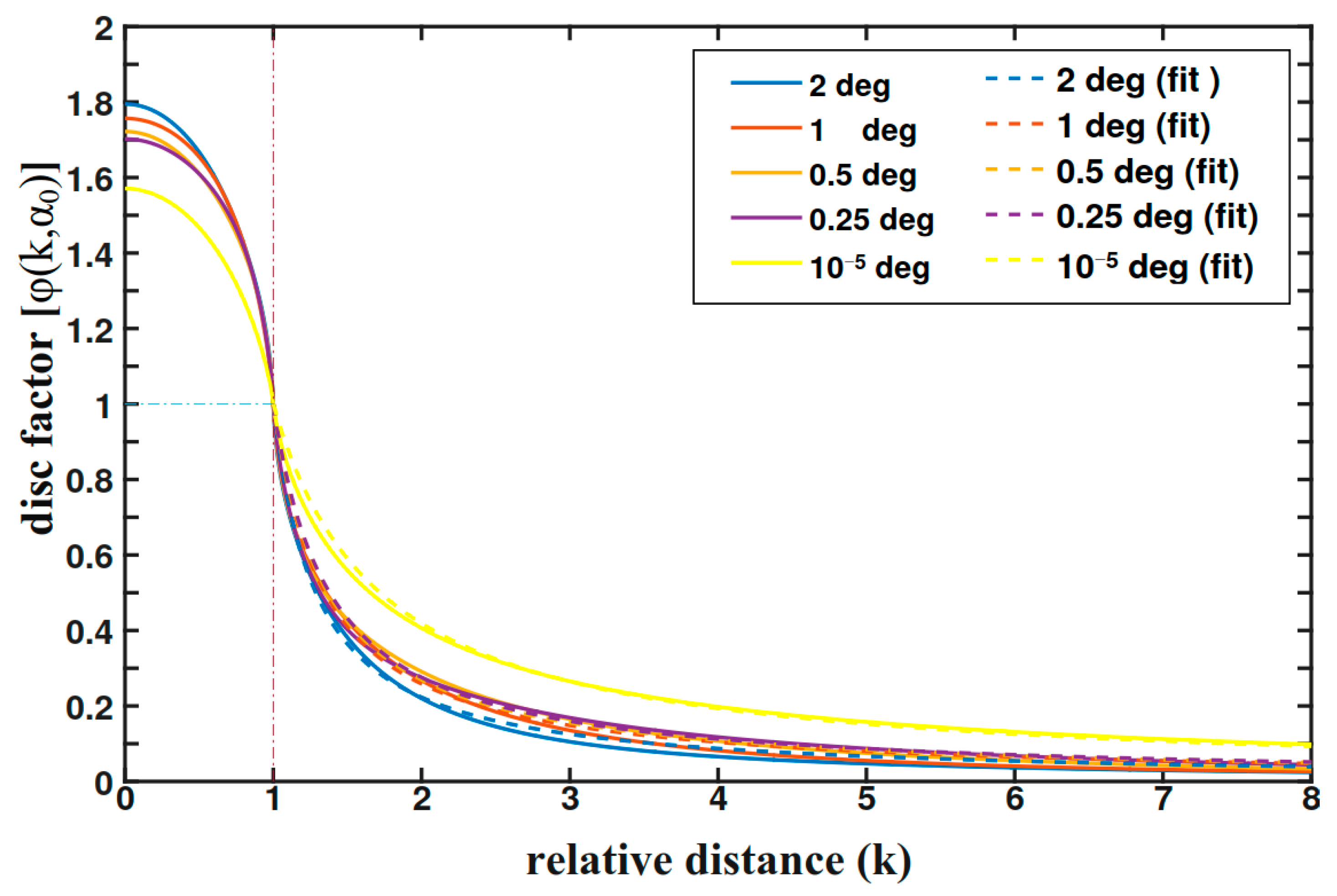The constraint parameters on$m_c$ and$G{\left(\alpha \right)}_c$are selected by the search radius${\alpha }_r$ which is determined by the DLEF model. Then, we inverse the water storage changes with the different search radius, i.e., three, five and seven times the radius of the net grid (3${\alpha }_0$, 5${\alpha }_0$and 7${\alpha }_0$), respectively; T4: similar to T2, but we add the grids’ vertical deformations of the outside study region (VD_out0) within 3${\alpha }_0$, 5${\alpha }_0$and 7${\alpha }_0$ from the study region boundary, and then repeat T1; T5: we repeat T4, the difference is that we add the Gauss white noise with 20% amplitude ratio (the noise can reach 20–30% of amplitude [26]) to each grid in or outside study region; T6: we use the part of the vertical deformations (VD₀ and VD_out0) which are at the real GPS sites distribution (un-uniform sites like in Figure 1) to invert the water storage changes, and then repeat T2 to T5. In T6, the vertical deformations in the outside region were also based on real GPS sites’ distribution as well.

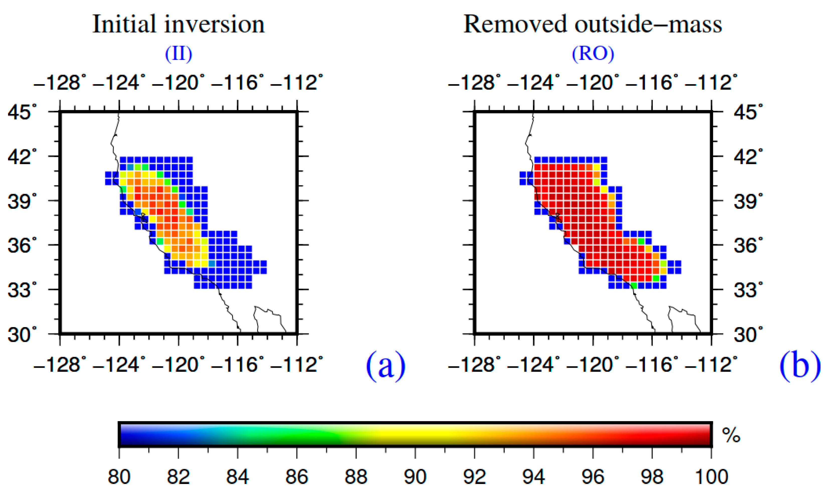
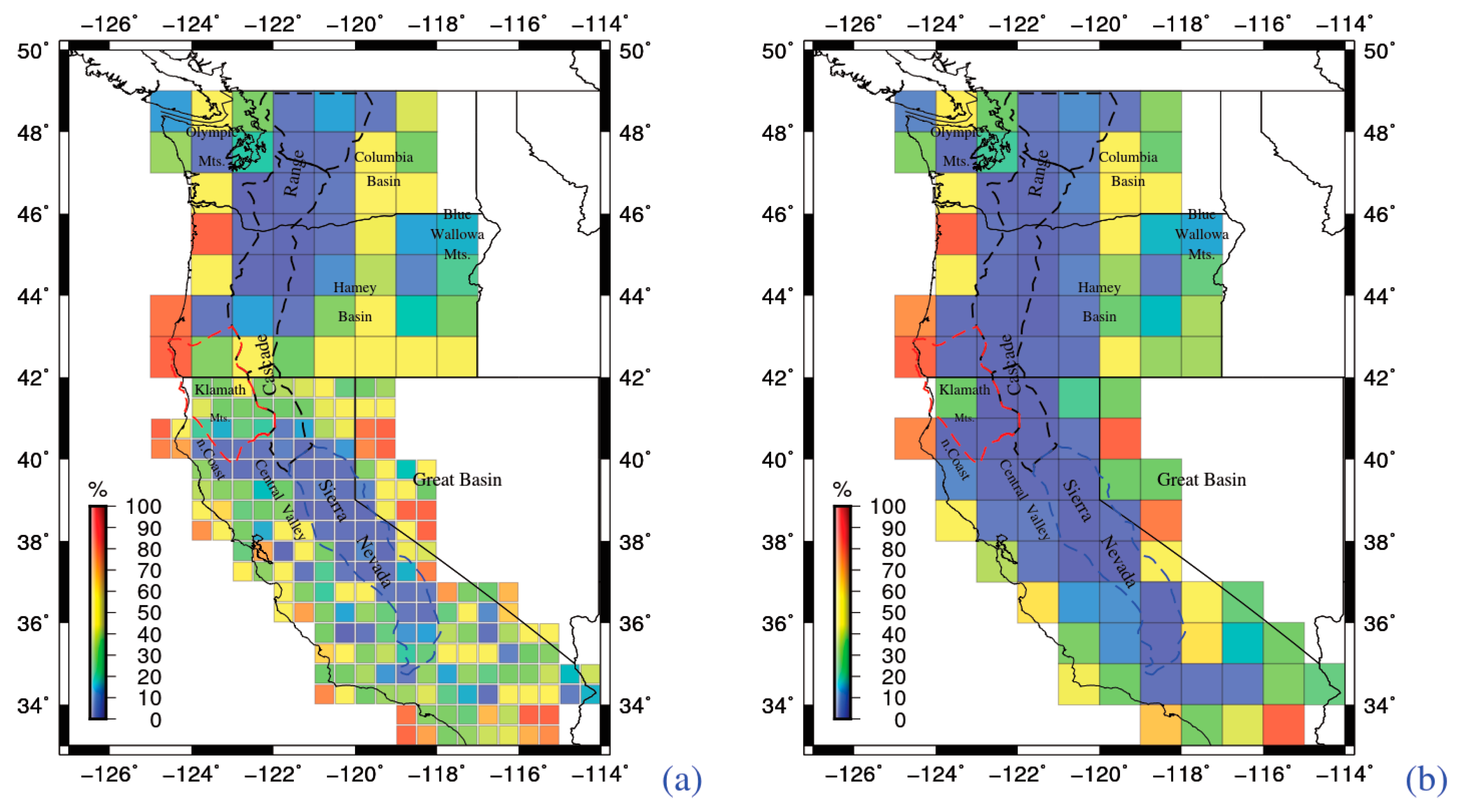
For case T1, only less than 30% of the inversion results (Figure 3a) have good agreements, i.e., VR greater than 90%, with the simulation water storage changes in California (the inversion spatial resolution is 0.5°), because the effect of the outside mass surrounding the study region have a large effect on the study region. Thus, the vertical deformations in the study region not only contain the water storage in the study region but are also influenced by outside mass variations. Furthermore, the agreement shows distinct spatial characteristics, and high VR (≥90%) in the center while low VR (≤90%, some even lower than ≤50%) in most boundary regions (Figure 3a). These T1 simulation results validate that the effect of mass outside of the study region must be considered.

We thus used the GRACE CSR Mascon product to remove the effect of large-scale mass outside the study region by Equation (1) in the case of T2 and then repeated T1. In this case, about 80% of the grids results have better agreement, i.e., VR is about 99%, with the simulation water storage changes. Unfortunately, other 20% grids’ results around the boundary regions still have worse VR (<80%) to compare with the central grids’ results (Figure 3b).

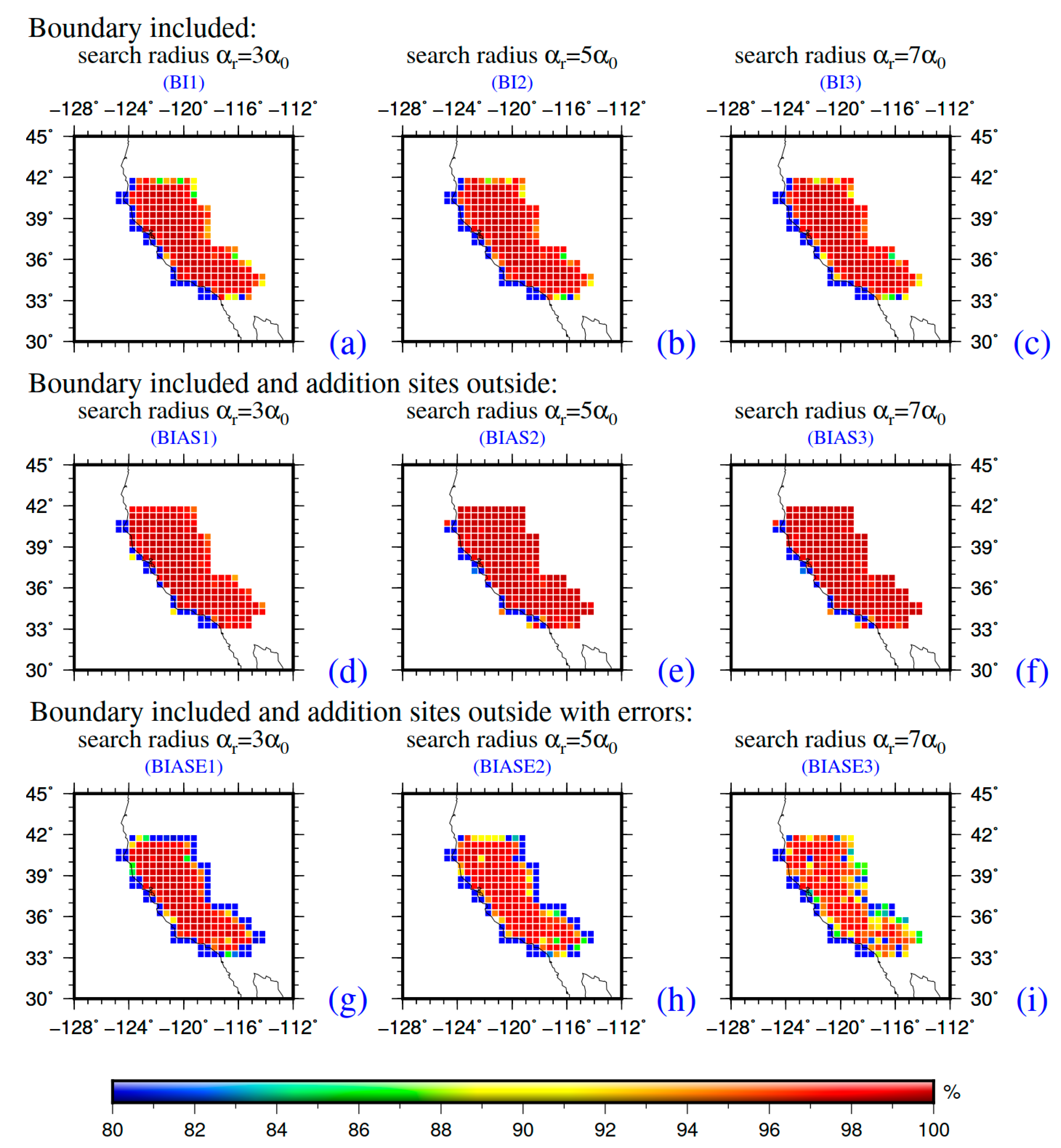
To overcome the aforementioned worse results in the boundary region, in case T3, we add the boundary included in the traditional inversion model, i.e., our new Equation (2b) model, with the Green function parameters$G{\left(\alpha \right)}_c$ to constrain on output parameter$m_c$. The new constraint results (Figure 4a) have obvious enhancement (VR > 90%) in the boundary regions, and in the center region, the new constrained results (Figure 4a) also have a small enhancement of about 1% in VR. Then, we try to change the boundary-included region, i.e., to set the search radius to be 5${\alpha }_0$ and 7${\alpha }_0$, respectively, and repeat the T3: the results show that more constraints have no obvious effect on the results’ enhancement, which is further evidence that choosing $3{\alpha }_0$ as the search radius is suitable enough in most cases ( Figure 4b,c).

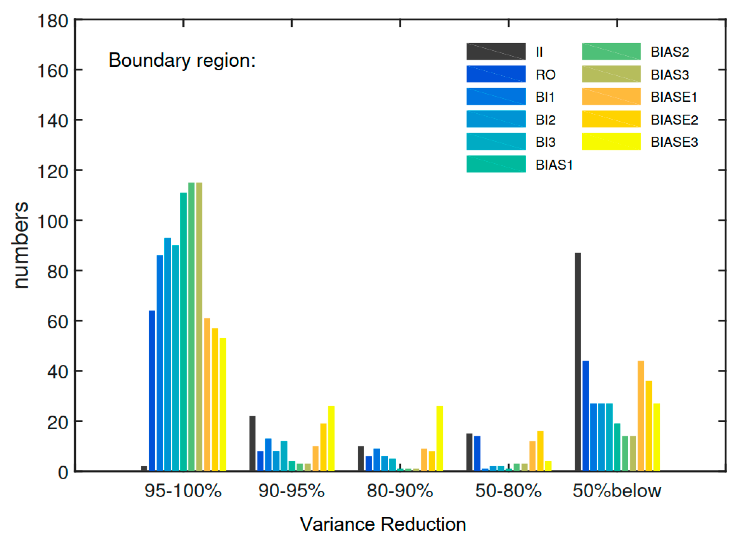
In case T4, we extended our study region with the additional outside vertical deformations; here, the inversion region is larger than the original study region, and its effect on the original boundary grids can be observed. The new study region is extended with 3${\alpha }_0$, 5${\alpha }_0$and 7${\alpha }_0$ from the original study region boundary, respectively. Subsequently, we used the T1 inversion method to invert the water storage in the original and outside study region. The inversion results indicate that in this case, we can get more accuracy results (VR > 95%, Figure 4d–f and Figure 5) at the original boundary grid and the extend area with a 3${\alpha }_0$ search radius which is good enough. Here, we notice that the inversion results are still bad (VR < 80%) in the coastal area, due to the fact that there is no extended value in the ocean and that the true value in these coastal areas tends to zero.

Generally, the errors of the GPS vertical deformations can reach the level of about 2–3 mm [26,27,28,29]. To mimic the case that the GPS deformations outside the study region have “errors”, we added the vertical deformations outside the study region with Gauss white noises of 20% amplitude ratio of that of the corresponding vertical deformations, and repeated T4. We called it the T5 case. The T5 results indicate that the Gauss white noises were brought into the inversion results, especially in the boundary regions (VR < 80% while in T4 VR > 95%), when the extended study region radius is the same as 3${\alpha }_0$. However, if the extended study region radius is extended to 5${\alpha }_0$or 7${\alpha }_0$, the VR at boundary grid have some increase from 80% to 90% but in the center grid decreased by about 5–10% (Figure 4g–i and Figure 5). Therefore, if the vertical deformations with errors in the outside study regions (this is almost the case in the real GPS data), our presented T3 results will have some obvious advantage to compare with that of T5. The similar conclusion can be seen in the Washington and Oregon sub-region (Figures S3–S5) too. Thus, our new boundary-included model of Equation (2b) will get better inversion results than the traditional method of Equation (2a) in this case.

Through the simulation tests T1–T5, we find that our boundary-included inversion model (Equation (2b)) can effectively improve the results by about 20% in the boundary regions. Actually, it was expected that there is another advantage for our new method in some special regions where there are no GPS observations outside but large effects from the UMC. Of course, the above T1–T5 simulations are all inverted from the uniform distributed vertical deformation, but in fact the real vertical deformations are usually observed by GPS sites with non-uniform spatial distribution. Therefore, we further design the simulation test T6, in which case the vertical deformations at the real GPS sites’ location but calculated from the NLDAS-Noah data are used to invert the regional water storage changes. 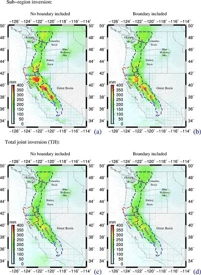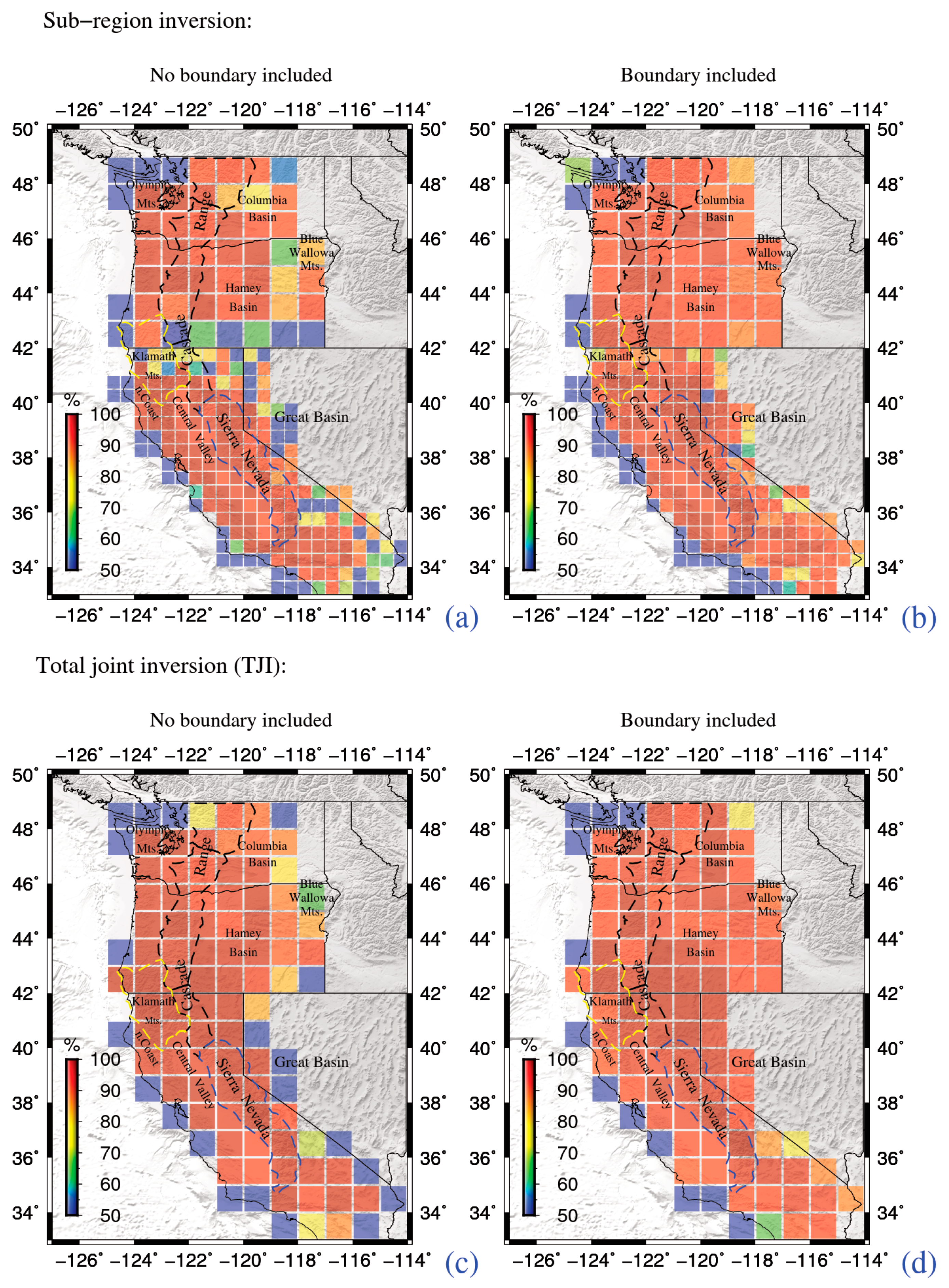Here, we only use 3 ${\alpha }_0$as the search radius to select the boundary-included constraint parameters. Because of the different spatial distribution of the GPS sites in the California sub-region and the Washington–Oregon sub-region, we inverted the water storage grid as 0.5° and 1° spatial resolutions in California and in Washington–Oregon, respectively, and independently. At the same time, we combined the above two study sub-regions as one (total joint inversion), i.e., the Pacific Rim of the western United States region, and inverted the water storage in the spatial resolution of 1°. All the inversion results indicate that the water storage VR in the boundary regions is enhanced with 10–20% (Figure 6). Even if we add outside vertical deformations without noises or with Gauss white noises as T4 or T5 as in the above inversion, the conclusions are still similar.

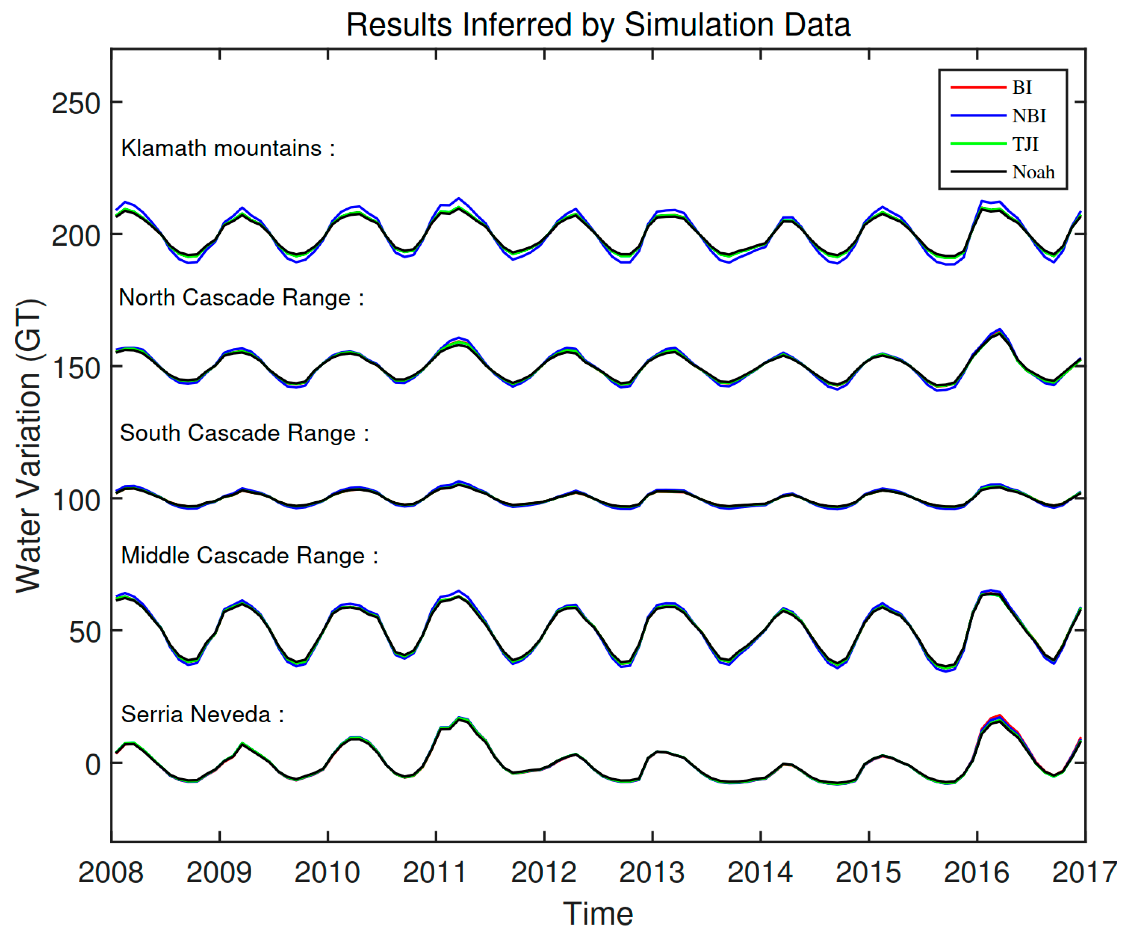
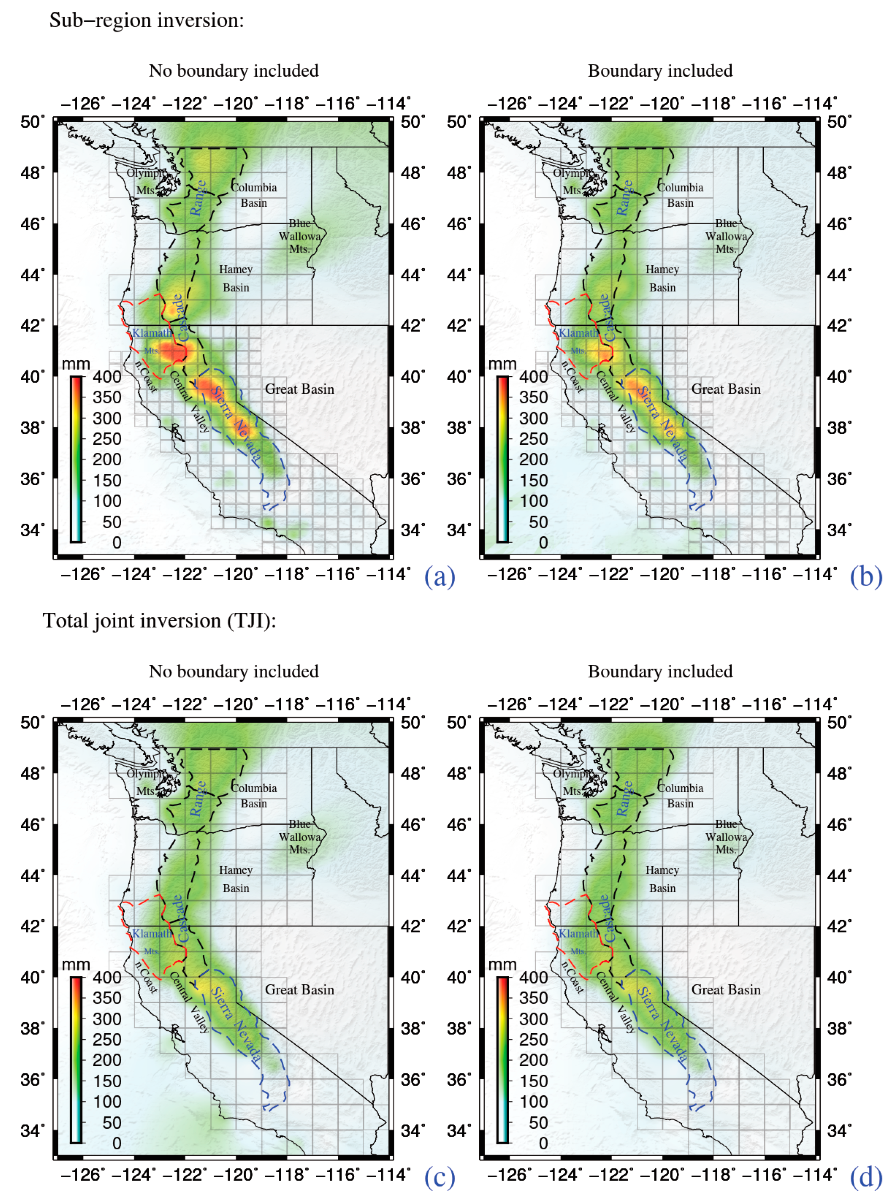
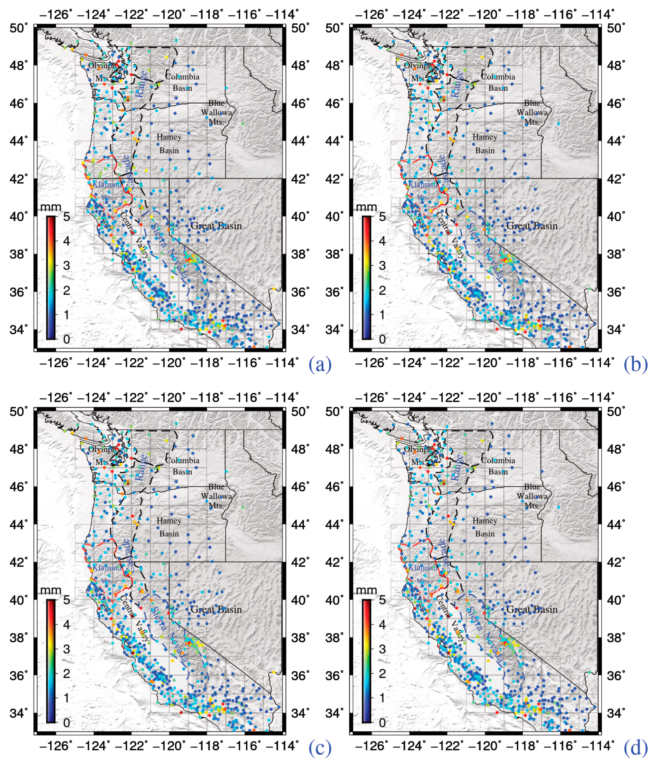
To further show our inversion results of T6 in more detail, we selected three physiographic provinces, i.e., Klamath mountains, Cascade Range, and Sierra Nevada, to compare the water storage time series between the inversion results and the original input of NLDAS-Noah, because in these regions, there are major water storage changes with clear seasonal signals of about 30–40 gt. The interesting thing is that these three regions denote different spatial characteristics. For example, when we use the California sub-region and Washington–Oregon sub-region for inversion, respectively, the physiographic province Klamath Mountains is in the boundary, Cascade Range has a small part in the boundary (e.g., north and south Cascade Range), and Sierra Nevada is in the center of the inversion region. Unquestionably, the results show that if the objective grids are in the center of the study region or only have limited boundary grids, our new model Equation (2b) will give little VR enhancement (0.2% in physiographic province Sierra Nevada and 1.9% in the physiographic province middle Cascade Range, Figure 7). However, if the inversion results are in the boundary regions, such as Klamath Mountains, north and south Cascade Range, these VR enhancements will be 14.3%, 9.7% and 7.6% (Figure 7), respectively, which indeed is a large improvement by our new model. If these physiographic provinces (Klamath Mountains, north and south Cascade Range) are all in the center of the study region (combine into only one big study region and invert it), all the inversion results in these three regions will fairly agree with the true value (NLDAS-Noah) (Figure 7).

Therefore, through these simulations (T1–T6), we validated that using the boundary-included inversion model Equation (2b) can improve the inversion result effectively in the boundary region. Then, we will show the water storage changes inverted from real GPS vertical deformation data by our presented model Equation (2b) in the Pacific Rim of the western United States.

3.2. Water Storage Changes Inverted from GPS Data

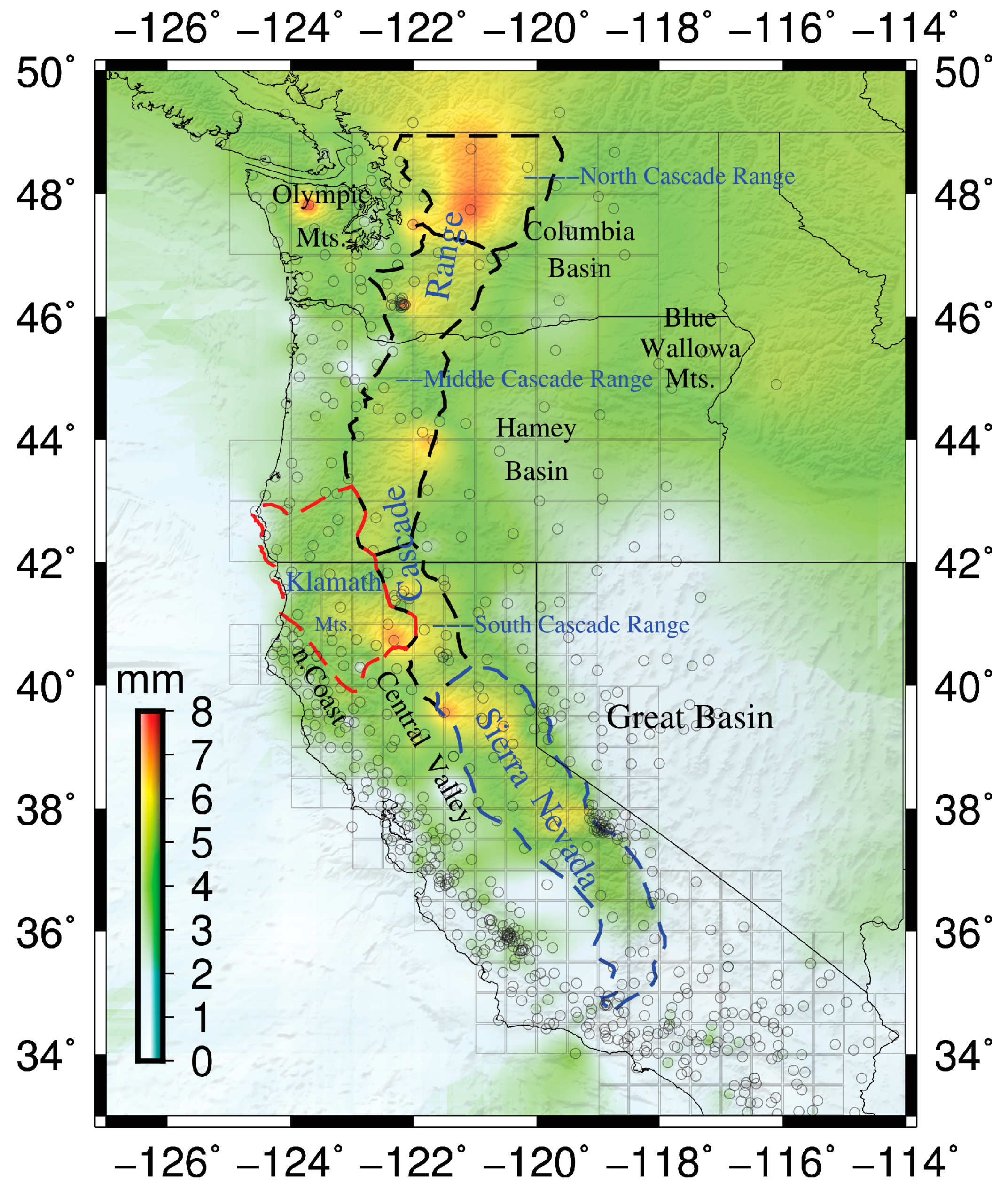
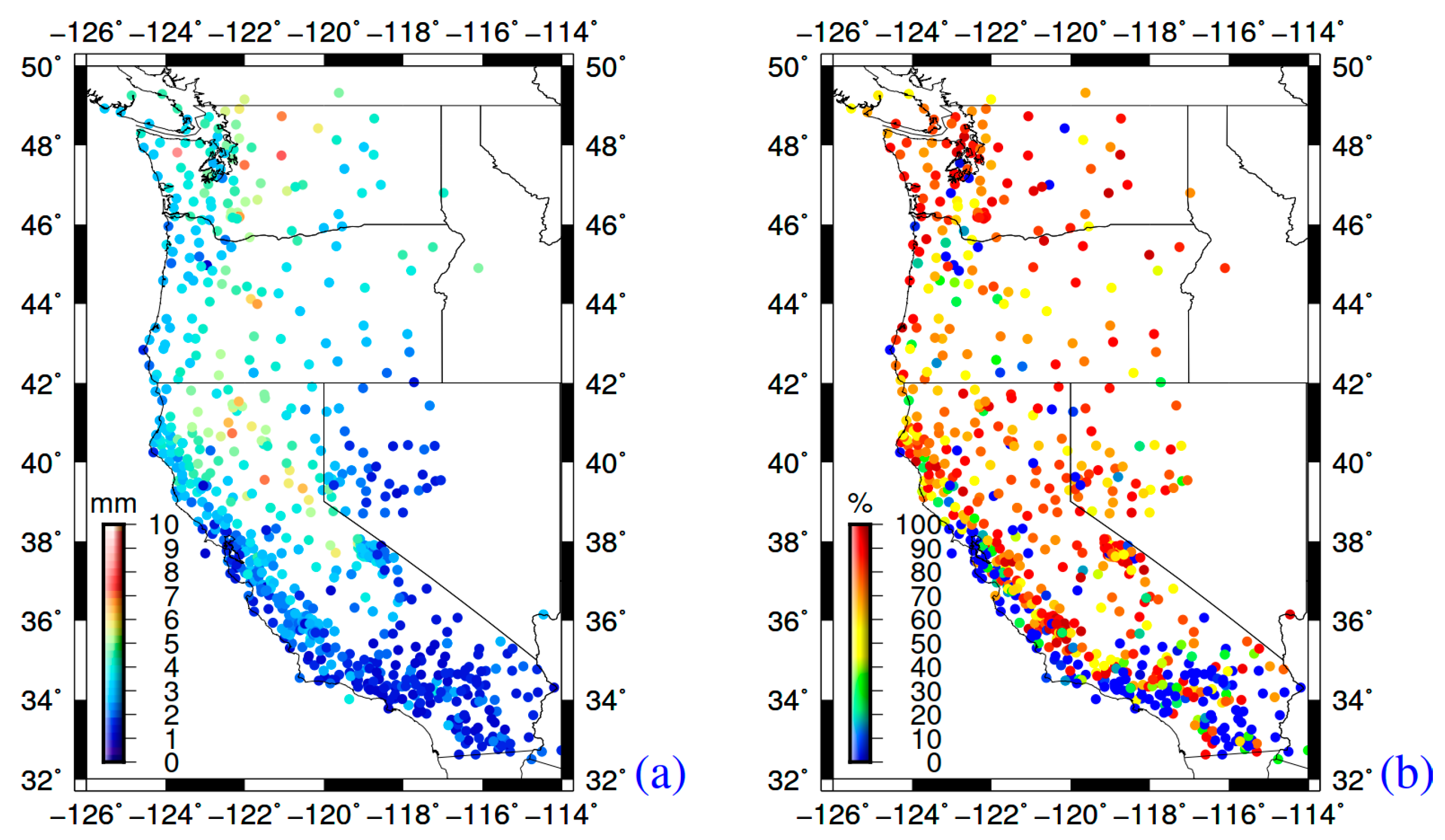
In the Pacific Rim of the western United States, there are a few GPS stations out of our study region and the annual vertical deformation amplitude of these GPS stations is generally smaller than 3 mm (Figure 1). Considering that the error level of the GPS vertical deformations is at the same level of 2–3 mm [26,27,28,29], we discard these outside region GPS observations due to the fact it could bring larger errors into inverted results, which was shown in T5 and T6. Meanwhile, we set the inversion spatial resolution of water storage changes as 0.5° × 0.5° in the California sub-region, 1° × 1° in the Washington–Oregon sub-region, and 1° × 1° for the whole study region, based on the numbers of the observed GPS stations in the different study regions (Figure 1 and Figure 8). At last, we set the search radius as 3${\alpha }_0$ (DLEF = 0.2), and inverted the water storage changes from such GPS vertical deformations.

The seasonal water storage changes in the western Unite States inverted from the GPS vertical deformation data show the obvious annual amplitudes generally larger than 300 mm in the Cascade Range, Klamath mountains, and Sierra Nevada (Figure 9). While in the valley and basin regions, such as Columbia and Harney Basin, the annual water storage amplitude is generally smaller than 100 mm. Our result is generally consistent with those from Argus et al. (2014) and Fu et al. (2015) in the spatial distribution characteristics.

Comparing the direct inversion results with that of the boundary-included inversion results (Figure 9a,b and Figure S6) separately, the direct inversion results are obviously larger than (about 50–80 mm in annual amplitudes) the boundary-included results in the boundary regions (e.g., Klamath Mountains, south Cascade Range and north Cascade Range ). However, in the center regions (e.g., Sierra Nevada and middle Cascade Range), the direct inversion results are similar with (about 10–30 mm larger in annual amplitudes) the boundary-included results. This is consistent with our simulation test results which show that the boundary included can only enhance about 1% of the VR in the center region. Meanwhile, the boundary-included water storage changes results, of 1° × 1° spatial resolution in the case of the Washington–Oregon sub-region, and 0.5° × 0.5° spatial resolution in the case of the California sub-region in the physiographic province Klamath Mountains (Figure 9b), are approximate to the direct inversion results in the same region (Figure 9c), where now as the center region of 1° × 1° spatial resolution in the case of the whole study region. This is consistent with our finding that the boundary-included results are more suitable than the direct inversion results, due to the latter critically overestimating the water storage changes in the boundary regions. Here, we also notice that in the boundary region, most of the direct inversion results are larger than those from boundary-included inversion. However, we still find that a few net grids’ water storages from direct inversion are smaller than that of the boundary-included inversion at the boundary of 0.5° × 0.5° spatial resolution in the case of the California sub-region, which may be sourced from the combined effect by GPS vertical deformations errors and the irregular space distribution of the GPS sites (some net grid of 0.5 × 0.5° spatial resolution has no GPS sites). For a better comparison between direct and boundary-included inversion results, we present the percentage of the residuals (between the two results) standard deviation to the boundary-included results standard deviation (more approximate to the true value than direct results) in Figure 8. Furthermore, we counted the number of the grids of which the percentage is greater than 20%. Here, we see the grids of which the percentage is greater than 20% as the significant difference grids which are clearly above the GPS vertical deformation errors level. For the 0.5° × 0.5° spatial resolution case study in the California sub-region and the 1° × 1° spatial resolution case study in the Washington–Oregon sub-region, there are 65% grids which are of significant difference (the percentage is greater than 20% in Figure 8). Moreover, for 1° × 1° in the whole study region, there are 47% grids which are of significant difference. It is obvious that these significant difference points are mainly located in the boundary region. Therefore, the boundary-included inversion can effectively improve the results when we use the GPS deformation to infer water storage changes. One may notice the difference between 65% and 47%. This is due to the grid number used in the different region especially in the boundary regions (e.g., Figure 8a,b).

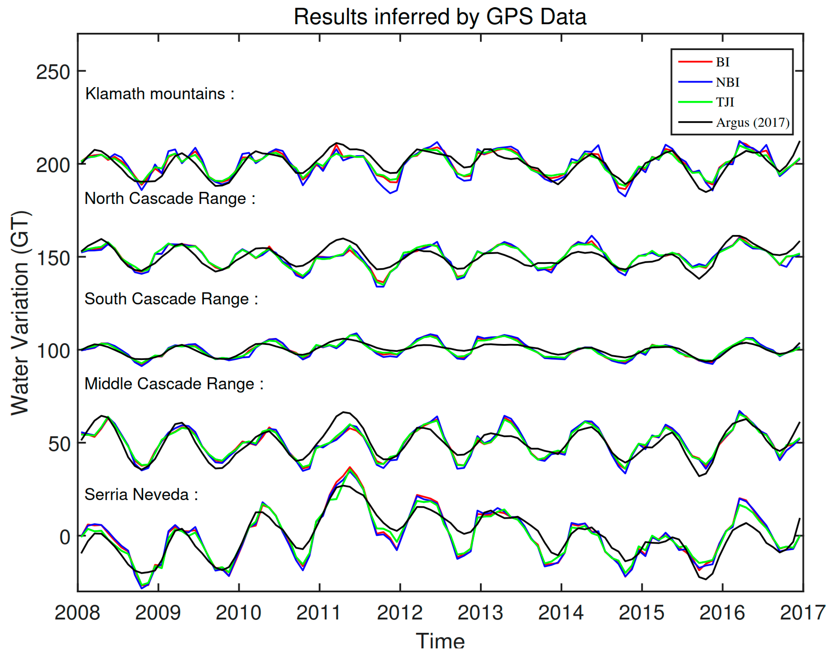
Furthermore, we compare the inverted total water storage changes by different inversion methods in three physiographic provinces, i.e., Klamath Mountains, Cascade Range and Sierra Nevada. Here, we take the total joint inversion results with the boundary included as the “true” value based on Section 3.1, which the spatial resolution of the water storage changes is 1° × 1° for the whole study region. Then, we use this “true” value as the standard to evaluate if the sub-region inversion results have significant enhancements with our boundary-included inversion method. In Figure 10, our boundary-included inversion results of the variance enhancement are about 16.0%, 11.4%, 9.5%, 2.1% and 0.5% in the Klamath Mountains (boundary region), north, south, and middle Cascade Range (north and south Cascade Range is the boundary region, most of middle Cascade Range is the inner region) and Sierra Nevada (inner region), respectively. The above results show that our boundary-included inversion method is powerful in the boundary regions, but similar to direct inversion results in the center region. This result is similar as our simulation test T6, which enhances the variance for about 14.3%, 9.7%, 7.6%, 1.9% and 0.2% in the similar case. We also notice that the enhancement (16.0%, 11.4% and 9.5%) of the inversion results with the boundary included by real GPS vertical deformation is slightly larger than that of the simulation results (14.3%, 9.7% and 7.6%), which further prove that the boundary-included inversion method has more advantages in the data with the true error environment.

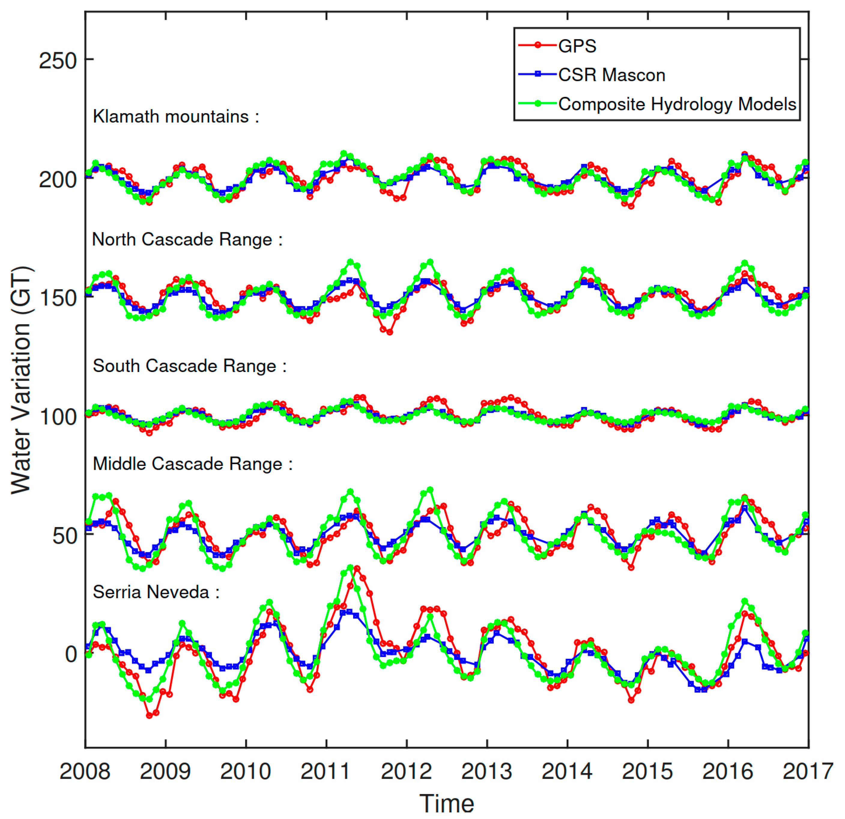
Finally, we compare our boundary-included inversion model results with the water storage changes derived from composite hydrology models [30] and the GRACE CSR Mascon product (Figure 11). The annual amplitude of the water storage changes by the different products (GRACE CSR Mascon, composite hydrology models, Argus et al. (2017) and our boundary-included model) in the physiographic provinces (Klamath Mountains, Cascade Range and Sierra Nevada) is shown in

Table 3. Annual amplitude of the water storage changes comparison of the different products.

Products	Annual Amplitude of the Water Storage Changes in Physiographic Provinces (Gt)
	Klamath Mountains	North Cascade Range	Middle Cascade Range	South Cascade Range	Sierra Nevada
GRACE CSR Mascon	5.4	5.1	6.3	2.8	7.1
Composite hydrology models	5.8	8.6	10.8	3.0	12.5
Argus et al. (2017)	6.7	5.7	9.3	2.7	9.1
Boundary-Included Model	6.6	7.2	9.5	3.1	12.3

. We that see our boundary-included model results are consistent with that of the composite hydrology models and Argus et al. (2017) on the whole. However, in the north Cascade Range (boundary region), the annual amplitude 7.2 Gt of our inversion results is slightly less than that of the composite hydrology model result of 8.6 Gt and larger than that of Argus et al. (2017)’s result of 5.7 Gt. Considering that most of the variance reduction between the vertical deformation calculated from composite hydrology models data and GPS vertical deformation can reach about 90% (Figure 12b), their inversion result in this boundary region may be slightly underestimated. Moreover, in Sierra Nevada (the center of the California sub-region where the GPS sites are denser), the annual amplitude 12.3 Gt of our inversion results is similar to that of the composite hydrology model result of 12.5 Gt and slightly larger than that of Argus et al. (2017)’s result of 9.1 Gt. Here, most of the variance reduction between the vertical deformation calculated from the composite hydrology models data and the GPS vertical deformation can reach above 90% (Figure 12b). Therefore, the smooth factor in the inversion model of Argus et al. (2017) may smooth the “local” water storage changes of the results, which may cause the slightly underestimated results for Sierra Nevada.

Furthermore, we noticed that the water storage changes inferred by the GPS vertical deformation are generally larger than that of the GRACE-CSR products (Figure 11 and Table 3). In addition, there is a slightly obvious difference between the water storage changes of the GPS vertical deformation inferred and the composite hydrological model. The reason is that the spatial resolution of the GRACE-CSR products is about 300 km, which is larger than that of the GPS vertical deformation and the composite hydrological models. Thus, the GRACE products can only show the “average” results in the 300 × 300 km spatial region, while the GPS and hydrological models can show more “local” results. Otherwise, the GPS vertical deformation signal has a lot of non-hydrological “errors”, such as orbit errors, thermal errors, monument errors, un-modeled troposphere and ionosphere errors, etc., which is not the true hydrology signal but taken as the hydrological signal. These “errors” will show as false local hydrological signals too. Composite hydrology models may have similar problems. These different “errors” in GRACE, GPS and hydrology models will cause the difference results between the directed or inverted water storage changes. Furthermore, we also notice that the phase of the water storage changes time series inferred by the GPS vertical deformations lags that of the hydrology models and GRACE-CSR products, obviously. This phase lag phenomenon is quite complex and important, and should be examined in the future.

4. Discussion

Our boundary-included inversion model can invert better water storage changes than the direct inversion model, especially in the boundary region, and in a robust way. It is very useful for water inversion in the mountain-plain joint area (e.g., North China region), coast region (e.g., western American), or big islands (e.g., Greenland and Japan), because there are substantial mass changes but we have few or even no GPS observations for these study regions.

However, our inversion model and the results presented here are based on the hypothesis that the water storage changes are roughly continue with a smooth spatial distribution in the study region. That is almost true for the above US study region, with about 50–100 km spatial resolution. If the water storage changes are discrete or the spatial resolution of the GPS station reaches the 1–10 km level, the GPS observations may be largely polluted by the local water changes. In this case, our Laplacian operator regularization method in Equation (2) should probably not be suitable. Thus, we should consider some other suitable regularization operator, such as normal 1 or normal ∝, to substitute our Laplacian operator in Equation (2).

Furthermore, to solve Equation (2), the balance between the numbers of GPS observations and constraint Green function parameters based on $m_c$ must be considered too. If the number of GPS observations in the study region is very scarce and we still want to have a better water storage inversion with better spatial resolution, we should decrease the constraint parameter numbers with stricter criterions than that of our model. For example, based on the other related observations, such as meteorological, well-based, geological, and geophysical observations, we can set the mass change as zero in the constraint grid. This can be done either by analyzing the above direct observations or by using some spatial statistical methods, such as Getis-ord Local G method [31,32], to judge the spatial correlation value and draw non-mass change grid maps, and thus decrease the constraint parameters‘ number.

Apart from the inversion methods chosen and the GPS spatial resolution problems, which can affect the final inversion accuracy of water storage changes, the source of most uncertainties during the water storage inversion from the observed GPS vertical deformations are the “errors” in the GPS vertical deformation itself. For example, Dong et al. (2002) showed that the GPS height changes include global and regional correlated errors, such as a priori modeling errors (e.g., tides, non-annual loadings, or loading model errors), other large-scale analysis errors (e.g., orbits) and local site-specific errors, such as multipath and monument noise, antenna miscalibration, troposphere and ionosphere mismodeling. The expansion and contraction of GPS stations monuments and nearby bedrock by thermal change can also be recorded in GPS vertical height. Yan et al. (2009) showed that the thermal contribution to GPS vertical height is up to a few mm level and can explain about 10% of the observed GPS variations. Furthermore, Yan et al. (2018) showed that the geophysical fluids can generally explain 70% of the observed GPS variance, which indicates that at least 30% of “errors” in the GPS observation cannot be removed correctly. We also use our inversion results to recalculate the load vertical deformations by Equation (1), and compare the deformations with the original GPS vertical deformations at each site. The standard deviations of the residuals between the recalculated vertical deformation and that of the observed one is shown in Figure 13. In the center region, the residuals’ standard deviations of most sites are about 1 mm and a few sites near the subsidence region (e.g., Central Valley) and volcanic region (e.g., Olympic mountains) can reach up to 3–5 mm in standard deviations. In the boundary region, the residuals’ standard deviations for the boundary-included inversion method are generally smaller than that of the direct inversion method, but usually at the 1–2 mm level which is less than the GPS error level. Thus, all the unremoved errors in the GPS vertical deformation data will be taken as the hydrological signal in the inversion process, which unquestionably brings the overestimate/underestimate of the final results of inverted water storage changes (e.g., Figure 10). In this sense, beyond the method, the most important thing in the accurate water storage changes’ inversion from the GPS vertical deformation is to remove all the possible non-water “errors” in the GPS observation clearly and previously. This must be based on our deep understanding of what signals are in the observed GPS vertical deformation time series.

5. Conclusions

In this paper, we presented a new boundary-included model to invert the water storage changes from the observed GPS vertical deformation in a robust way in the Pacific Rim of the western United States. The key point of our boundary-included inversion model is to determine the boundary-included constraint parameters by our developed DLEF model, which uses the theoretic disc load to obtain an appropriate search radius to determine the boundary-included constraint parameters. We then validated our method in a series of simulations. The results of the simulation tests indicate that our boundary-included inversion model can effectively improve 10–20% of the variance of the inversion results in the boundary regions. For the inversion results from the real GPS vertical deformation, we show that our inverted water storage changes in the boundary regions are approximate to the hydrological model and GRACE products, and are about 10–20% in variance better than that of the traditional direct inversion method. However, we also notice that the deformation from the observed GPS vertical deformation is prone to be contaminated by a lot of error sources. Therefore, to infer more accurate water storage changes by GPS vertical deformation data, we should improve not only the inversion model, but also more accurately separate the hydrological load signal from the GPS observations.

References

1. Tapley, B.D.; Bettadpur, S.; Watkins, M.; Reigber, C. The gravity recovery and climate experiment: Mission overview and early results. Geophys. Res. Lett. 2004, 31. [Google Scholar] [CrossRef] [Green Version]
2. Eicker, A.; Schumacher, M.; Kusche, J.; Döll, P.; Schmied, H.M. Calibration/Data Assimilation Approach for Integrating GRACE Data into the WaterGAP Global Hydrology Model (WGHM) Using an Ensemble Kalman Filter: First Results. Surv. Geophys. 2014, 35, 1285–1309. [Google Scholar] [CrossRef]
3. Zaitchik, B.F.; Rodell, M.; Reichle, R.H. Assimilation of GRACE Terrestrial Water Storage Data into a Land Surface Model: Results for the Mississippi River Basin. J. Hydrometeorol. 2008, 9, 535–548. [Google Scholar] [CrossRef]
4. Borsa, A.A.; Agnewand, D.C.; Cayan, D.R. Ongoing drought-induced uplift in the western United States. Science 2014, 345, 1587–1590. [Google Scholar] [CrossRef]
5. Argus, D.F.; Yuning, F.; Landerer, F.W. Seasonal variation in total water storage in California inferred from GPS observations of vertical land motion. Geophys. Res. Lett. 2014, 41, 1971–1980. [Google Scholar] [CrossRef]
6. Fu, Y.; Argus, D.F.; Landerer, F.W. GPS as an independent measurement to estimate terrestrial water storage variations in Washington and Oregon. J. Geophys. Res. Solid Earth 2015, 120, 552–566. [Google Scholar] [CrossRef]
7. Argus, D.F.; Landerer, F.W.; Wiese, D.N.; Martens, H.R.; Fu, Y.; Famiglietti, J.S.; Thomas, B.F.; Farr, T.G.; Moore, A.W.; Watkins, M.M. Sustained Water Loss in California’s Mountain Ranges During Severe Drought from 2012 to 2015 Inferred from GPS. J. Geophys. Res. Solid Earth 2017, 122. [Google Scholar] [CrossRef] [Green Version]
8. Farrell, W.E. Deformation of the Earth by surface loads. Rev. Geophys. 1972, 10, 761–797. [Google Scholar] [CrossRef]
9. Blewitt, G.; Lavallée, D.; Clarke, P.; Nurutdinov, K. A New Global Mode of Earth Deformation: Seasonal Cycle Detected. Science 2001, 294, 2342–2345. [Google Scholar] [CrossRef] [Green Version]
10. Bevis, M.; Alsdorf, D.; Kendrick, E.; Fortes, L.P.; Forsberg, B.; Smalley, R., Jr.; Becker, J. Seasonal fluctuations in the mass of the Amazon River system and Earth’s elastic response. Geophys. Res. Lett. 2005, 32, L16308. [Google Scholar] [CrossRef] [Green Version]
11. Scripps Orbit and Permanent Array Center (SOPAC). Available online: http://sopac-ftp.ucsd.edu/pub/timeseries/measures/ats/WesternNorthAmerica/ (accessed on 5 May 2018).
12. Zumberge, J.F.; Heflin, M.B.; Jefferson, D.C.; Watkins, M.M.; Webb, J.F.H. Precise point positioning for the efficient and robust analysis of GPS data from large networks. J. Geophys. Res. 1997, 102, 5005–5017. [Google Scholar] [CrossRef] [Green Version]
13. Desai, S.D.; Bertiger, W.; Haines, B.; Harvey, N.; Selle, C.; Sibthorpe, A.; Weiss, J.P. Results from the reanalysis of global GPS data in the IGS08 reference frame. In Proceedings of the American Geophysical Union Fall Meeting 2011, San Francisco, CA, USA, 5–9 December 2011. [Google Scholar]
14. Schmid, R.; Steigenberger, P.; Gendt, G.; Ge, M.; Rothacher, M. Generation of a consistent absolute phase-center correction model for GPS receiver and satellite antennas. J. Geod. 2007, 81, 781–798. [Google Scholar] [CrossRef] [Green Version]
15. Sibthorpe, A.; Weiss, J.P.; Harvey, N.; Kuang, D.; Bar-Sever, Y. Empirical modeling of solar radiation pressure forces affecting GPS satellites. In Proceedings of the American Geophysical Union Fall Meeting 2011, San Francisco, CA, USA, 5–9 December 2011. [Google Scholar]
16. Petit, G.; Luzum, B.E. IERS technical note 36. In IERS Conventions (2010); Verlag des Bundesamts für Kartographie und Geodäsie: Frankfurt, Germany, 2010; Volume 111, p. 179. [Google Scholar]
17. Dong, D.; Fang, P.; Bock, Y.; Webb, F.; Prawirodirdjo, L.; Kedar, S.; Jamason, P. Spatiotemporal filtering using principal component analysis and Karhunen-Loeve expansion approaches for regional GPS network analysis. J. Geophys. Res. Solid Earth 2006, 111. [Google Scholar] [CrossRef] [Green Version]
18. Dee, D.P.; Uppala, S.M.; Simmons, A.J.; Berrisford, P.; Poli, P.; Kobayashi, S.; Andrae, U.; Balmaseda, M.A.; Balsamo, G.; Bauer, D.P.; et al. The ERA-Interim reanalysis: Configuration and performance of the data assimilation system. Q. J. R. Meteorol. Soc. 2011, 137, 553–597. [Google Scholar] [CrossRef]
19. Estimating the Circulation and Climate of the Ocean (ECCO). Available online: https://http//ecco.jpl.nasa.gov/thredds/las/kf080/catalog.html/ (accessed on 5 May 2018).
20. Wang, H.; Xiang, L.; Jia, L.; Jiang, L.; Wang, Z.; Hu, B.; Gao, P. Love numbers and Green’s functions for elastic Earth models PREM. iasp91 2012, ak135, and modified models with refined crustal structure from Crust 2.0. Comput. Geosci. 2012, 49, 190–199. [Google Scholar] [CrossRef]
21. Save, H.; Bettadpur, S.; Tapley, B.D. High resolution CSR GRACE RL05 mascons. J. Geophys. Res. Solid Earth 2016, 121, 7547–7569. [Google Scholar] [CrossRef]
22. Harris, R.A.; Segall, P. Detection of a locked zone at depth on the Parkfield. California, segment of the San Andreas Fault. J. Geophys. Res. Solid Earth 1987, 92, 7945–7962. [Google Scholar] [CrossRef]
23. O’Leary, D.P.; Hansen, P.C. The Use of the L-Curve in the Regularization of Discrete Ill-Posed Problems. SIAM J. Sci. Comput. 1993, 14, 1487–1503. [Google Scholar]
24. Tregoning, P.; Watson, C.; Ramillien, G.; McQueen, H.; Zhang, J. Detecting hydrologic deformation using GRACE and GPS. Geophys. Res. Lett. 2009, 36, L15401. [Google Scholar] [CrossRef] [Green Version]
25. Van Dam, T.; Wahr, J.; Lavallée, D. A comparison of annual vertical crustal displacements from GPS and Gravity Recovery and Climate Experiment (GRACE) over Europe. J. Geophys. Res. Solid Earth 2007, 112, B03404. [Google Scholar] [CrossRef] [Green Version]
26. Yan, H.; Chen, W.; Yuan, L. Crustal vertical deformation response to different spatial scales of grace and gcms surface loading. Geophys. J. Int. 2018, 204, 505–516. [Google Scholar] [CrossRef] [Green Version]
27. Yan, H.; Chen, W.; Zhu, Y.; Zhang, W.; Zhong, M. Contributions of thermal expansion of monuments and nearby bedrock to observed GPS height changes. Geophys. Res. Lett. 2009, 36, 88–97. [Google Scholar] [CrossRef] [Green Version]
28. Ray, J.; Collilieux, X.; Rebischung, P.; van Dam, T.M.; Altamimi, Z. Consistency of crustal loading signals derived from models and GPS: Inferences for GPS positioning errors. In Proceedings of the American Geophysical Union Fall Meeting 2011, San Francisco, CA, USA, 5–9 December 2011; Available online: acc.igs.org/trf/pos-errs_agu-f11.ppt (accessed on 7 December 2018).
29. Valty, P.; de Viron, O.; Panet, I.; Van Camp, M.; Legrand, J. Assessing the precision in loading estimates by geodetic techniques in Southern Europe. Geophys. J. Int. 2013, 194, 1441–1454. [Google Scholar] [CrossRef]
30. Argus, D.F.; Landerer, F.W.; Wiese, D.N.; Martens, H.R.; Fu, Y.; Famiglietti, J.S.; Thomas, B.F.; Farr, T.G.; Moore, A.W. Soil Moisture Data in the NLDAS-Noah Model, the Snow Water Equivalent in the Snow Data Assimilation System and the Reservoirs Data. 13 June 2019. Available online: ftp://garner.ucsd.edu/pub/projects/eseses.2019/ (accessed on 1 May 2020).
31. Anselin, L. Local indicators of spatial association—LISA. Geogr. Anal. 1995, 27, 93–115. [Google Scholar] [CrossRef]
32. Ord, J.K.; Getis, A. Local spatial autocorrelation statistics: Distributional issues and an application. Geogr. Anal. 1995, 27, 286–306. [Google Scholar] [CrossRef]
Figure 1. The stations’ distribution and their annual amplitude of vertical deformation (the values of the base map are interpolated by the Generic Mapping Tools (GMT) tool using the annual amplitude). Here, the California sub-region is south latitude 42° of the west Pacific Rim region, and the Washington and Oregon sub-region is north latitude 42° of the west Pacific Rim region. Physiographic provinces Klamath Mountains, Cascade Range and Sierra Nevada are from Argus et al. (2017).
Remotesensing 12 02429 g001
Figure 2. The line data obtained by integrating the vertical deformation Green function across the discs of several radii α 0 (degrees) centered at various distances α . The relative distance ( k ) is α / α 0 , and the disc factor is the integral u ( α ) divide by u ( α 0 ) . The dotted line is the disc load empirical function φ ( k , α 0 ) .
Remotesensing 12 02429 g002
Figure 3. The inversion result of the simulation vertical deformations (with uniform 0.25° × 0.25° distribution) in California (0.5° inversion spatial resolution). The outside mass effect is not removed in (a), while the outside mass is removed by Gravity Recovery and Climate Experiment (GRACE) Center for Space Research (CSR) Mascon data in (b).
Remotesensing 12 02429 g003
Figure 4. The inversion spatial resolution is 0.5 in California. (ac) are the inversion results of the simulation test T3 (the search radius is 0.75°, 1.25 °and 1.75°); (df) are the inversion results of the simulation test T4 (the extended area is 0.75°, 1.25 °and 1.75° and the additional vertical deformations with no errors); (gi) are the inversion results of the simulation test T5n (the extended area is 0.75°, 1.25°and 1.75°and the additional vertical deformations with 20% amplitude ratio Gauss white noise).
Remotesensing 12 02429 g004
Figure 5. Histogram by the variance reduction of the simulation inversion results (Figure 3 and Figure 4) with true value in the boundary region.
Remotesensing 12 02429 g005
Figure 6. The result of the simulation test T6. The spatial resolution is 1° north of the latitude 42° N line, and the spatial resolution is 0.5° south of the latitude 42° N line in (a,b); (c,d) use the total joint inversion and the spatial resolution is 1°; (a,c) are with no boundary included; (b,d) are with boundary included.
Remotesensing 12 02429 g006
Figure 7. The time series of the simulation inversion results within Klamath Mountains, Cascade Range and Sierra Nevada. The red line is the results with the boundary included of sub-region inversion (BI); the blue line is the results with no boundary included of sub-region inversion (NBI); the green line is the results that use the total joint inversion with boundary included (TJI); the black line is the data from NLDAS-Noah (Noah).
Remotesensing 12 02429 g007
Figure 8. The percentage of the standard deviation of the residuals (between the boundary-included results and the no boundary-included results) to the boundary-included results’ standard deviation. The spatial resolution is 1° north of the latitude 42° N line, and the spatial resolution is 0.5° south of the latitude 42° N line in (a); the inversion spatial resolution of the whole region is 1° in (b).
Remotesensing 12 02429 g008
Figure 9. The result inferred by the real GPS vertical deformation. All the experiments have removed the outside mass by GRACE CSR Mascon data. The spatial resolution is 1° north of the latitude 42° N line, and the spatial resolution is 0.5° south of the latitude 42° N line in (a,b); (c,d) use the total joint inversion and the inversion spatial resolution is 1°; (a,c) are with no boundary included; (b,d) are with boundary included; the Kriging interpolation was used in this spatial distribution figure.
Remotesensing 12 02429 g009
Figure 10. The time series of the real GPS vertical deformation inversion results within the Klamath Mountains, Cascade Range and the Sierra Nevada regions. The red line is the results with the boundary included; the blue line is the results with no boundary included; the green line is the results that use the total joint inversion with the boundary included; the black line is the results from Argus et al. (2017). All of the results used the detrend function from Matlab tools to study the seasonal changes.
Remotesensing 12 02429 g010
Figure 11. The storage variations within the Klamath Mountains, Cascade Range and Sierra Nevada inferred from the GPS monthly time series; and the comparisons with the GRACE CSR Mascon, composite hydrology models.
Remotesensing 12 02429 g011
Figure 12. The figure (a) shows the annual amplitude of the GPS vertical deformation; the right figure (b) shows the variance reduction of the vertical deformation by the composite hydrology model to the GPS vertical deformation (removed the atmosphere and OBP).
Remotesensing 12 02429 g012
Figure 13. Figure (a,c) show the standard deviation of the residuals between the vertical deformation (calculated by direct inversion results) with GPS vertical deformation; Right figure (b,d) show the standard deviation of the residuals between the vertical deformation (calculated by boundary-included inversion results) with GPS vertical deformation. Here, in (a,b), the inversion spatial resolution as 0.5° × 0.5° in the California sub-region and 1° × 1° in the Washington–Oregon sub-region; in (c,d), the inversion spatial resolution as 1° × 1° for the whole study region.
Remotesensing 12 02429 g013