Article

Monitoring Forest Infestation and Fire Disturbance in the Southern Appalachian Using a Time Series Analysis of Landsat Imagery

1
Department of Geography, Indiana University Bloomington, Bloomington, IN 47405, USA
2
Department of Civil and Environmental Engineering, Yonsei University, Seoul 03722, Korea
3
US Department of Agriculture Forest Service, Southern Research Station, Asheville, NC 28804, USA
4
Department of Geography, University of North Carolina at Chapel Hill, Chapel Hill, NC 27514, USA
*
Author to whom correspondence should be addressed.
Remote Sens. 2020, 12(15), 2412; https://doi.org/10.3390/rs12152412
Submission received: 17 June 2020 / Revised: 20 July 2020 / Accepted: 24 July 2020 / Published: 28 July 2020

Abstract

:
The southern Appalachian forests have been threatened by several large-scale disturbances, such as wildfire and infestation, which alter the forest ecosystem structures and functions. Hemlock Woolly Adelgid (Adelges tsugae Annand, HWA) is a non-native pest that causes widespread foliar damage and eventual mortality, resulting in irreversible tree decline in eastern (Tsuga canadensis) and Carolina (T. caroliniana) hemlocks throughout the eastern United States. It is important to monitor the extent and severity of these disturbances over space and time to better understand their implications in the biogeochemical cycles of forest landscapes. Using all available Landsat images, we investigate and compare the performance of Tasseled Cap Transformation (TCT)-based indices, Normalized Difference Vegetation Index (NDVI), Enhanced Vegetation Index (EVI), and Disturbance Index (DI) in capturing the spectral-temporal trajectory of both abrupt and gradual forest disturbances (e.g., fire and hemlock decline). For each Landsat pixel, the temporal trajectories of these indices were fitted into a time series model, separating the inter-annual disturbance patterns (low frequency) and seasonal phenology (high frequency) signals. We estimated the temporal dynamics of disturbances based on the residuals between the observed and predicted values of the model, investigated the performance of all the indices in capturing the hemlock decline intensity, and further validated the results with the number of individual dead hemlocks identified from high-resolution aerial images. Our results suggested that the overall performance of NDVI, followed by TCT wetness, was most accurate in detecting both the disturbance timing and hemlock decline intensity, explaining over 90% of the variability in the number of dead hemlocks. Despite the overall good performance of TCT wetness in characterizing the disturbance regime, our analysis showed that this index has some limitations in characterizing disturbances due to its recovery patterns following infestation.

Graphical Abstract

1. Introduction

Over the last century, due to climate change and human activities the eastern North American forests have been affected by a number of large-scale disturbances, including wildfires, insect infestation, frequent droughts, and human-induced deforestation [1,2,3]. Among these, non-native pests and wildfires have been reported as two major forest disturbance agents in the southern Appalachian Mountains [4,5]. Hemlock Woolly Adelgid (Adelges tsugae Annand, HWA) is a non-native insect that causes widespread foliar damage and potentially complete mortality [6,7] in eastern (Tsuga canadensis) hemlock and Carolina hemlock (Tsuga caroliniana) (hereafter, “hemlocks” refers to both species). Hemlocks are one of the key late successional species in this forest ecosystem which suppresses hardwood regeneration due to the cool shaded environments under the canopy [8]. Hemlocks usually occur in riparian areas and the moist coves of mixed forests in complex terrains [9], often co-occurring with Rhododendron understories [6,10,11]. Since the initial outbreak of HWA in Virginia in the early 1950s [12,13,14], HWA expanded and recently it has caused widespread hemlock decline in the southern Appalachians [7,9,15,16]. Due to the lack of natural controls such as predator insects and lethal cold temperature [10,17], complete hemlock mortality usually occurs over 4 to 6 years after the initial infestation in this region [12,18,19].
Fire regimes in the eastern US are characterized by frequent, low-intensity fires caused by both humans and natural causes [20,21]. Historically, the fire regime has contributed to the dominance of the fire-tolerant oak (Quercus) species in deciduous forests [22,23]. However, fire suppression since the “Smokey Bear” era has promoted a gradual decline in fire-tolerant oaks and increase in fire-sensitive mesophytic species (e.g., red maple and tulip poplar), often referred to as forest “mesophication” [20].
Altered by disturbances, the subsequent forest declines caused by fire, infestation, and recovery have both long- and short-term impacts on the forest composition and associated ecohydrological processes [7,24,25,26]. To better understand the implications of HWA infestation and fires in forest landscapes, the spatial pattern and severity of these disturbances needed to be accurately monitored over time [27]. Improvement in the monitoring of HWA defoliation and its progress in space and time can provide forest managers with a better understanding of the decline patterns, as well as post-defoliation restoration strategies [7,10]. However, the extensive scales of hemlock infestation have limited ground-based assessment and necessitate the use of multi-temporal aerial and satellite imagery for monitoring [19,28]. Remote sensing has been widely used to develop cost-effective and accurate approaches to monitor the forest defoliation across the eastern United States at different spatial scales [19,29,30,31]. Landsat imagery, in particular, provides the temporal and spatial information needed for monitoring and characterizing forest disturbances at the regional to continental scales [32,33,34,35,36,37,38,39].
Traditionally, the spatial distribution of disturbances was estimated by comparing a limited number of images before and after disturbances [15,27,40,41,42]. Forest disturbance outbreaks often lead to a major reduction in foliar biomass and greenness. Therefore, spectral vegetation indices (VIs) such as the Normalized Difference Vegetation Index (NDVI) [43,44] have been widely used in forest disturbance studies [27,41,45,46,47]. However, some studies suggested that the performance of some VIs could be limited by the rapid growth of co-occurring understory species and the regeneration of new seedlings [15,27]. Net canopy loss often accompanies changes in the light and soil moisture available for the recovery of new seedlings and faster growth of co-occurring species [3,10,48]. Therefore, Tasseled Cap transformation (TCT) indices [49] were also used in vegetation monitoring, such as fire, mortality, forest succession, and regeneration process, to detect the accompanying changes in forest conditions [15,38,42,50,51,52,53]. TCT usually incorporates three orthogonal principal components of brightness (TCB), greenness (TCG), and wetness (TCW) in a linear combination of multi-spectral bands [49]. Studies suggested that TCW, a shortwave infrared-dominated index, could be a reliable indicator of species health and structural complexity, highly correlated with the water content variation in vegetation and soil [15,38,52,54,55]. For example, Jones et al. [15] used two Landsat TM images to compare the NDVI and TCT indices’ performances, suggesting that the TCW differential index was strongly correlated with hemlock decline. Using Landsat images, Healey et al. [42] developed the Disturbance Index (DI), a linear combination of normalized TCT indices, to investigate stand-replacing forest changes.
There are still some limitations in using a small number of before- and after-disturbance images: First, this method can limit the understanding of the disturbance progress and subsequent recovery patterns over time [56]. Second, although this approach can be a good indicator of abrupt changes such as wildfire, it may have limited capability in detecting gradual disturbances, such as gradual defoliation or tree mortality [36]. Third, finding a pair of cloud-free near anniversary images to minimize the incidental changes is often challenging [39]. With the availability of all Landsat archived images [57], many studies used multi-temporal Landsat data to detect long-term changes in the land cover and forest structures [36,58,59,60]. These studies showed that using dense time series Landsat images is a powerful approach to characterize both abrupt and subtle disturbances [36,37,38,56,61,62,63,64].
However, it is not clear how well the dense time series of different spectral measurements work for monitoring abrupt and gradual damage in forest ecosystems. In this study, we aim to quantify the performance of different spectral indices derived from Landsat imagery in capturing the spectral-temporal characteristics of both gradual and abrupt forest disturbances by HWA infestation and fire. Our findings provide valuable guidance for future efforts monitoring forest ecosystem disturbance using remote sensing, and the algorithm we developed here can be used as an efficient tool for forest management, planning, and restoration.

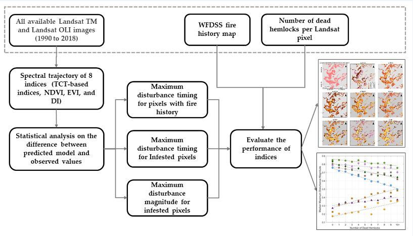
2. Materials and Methods
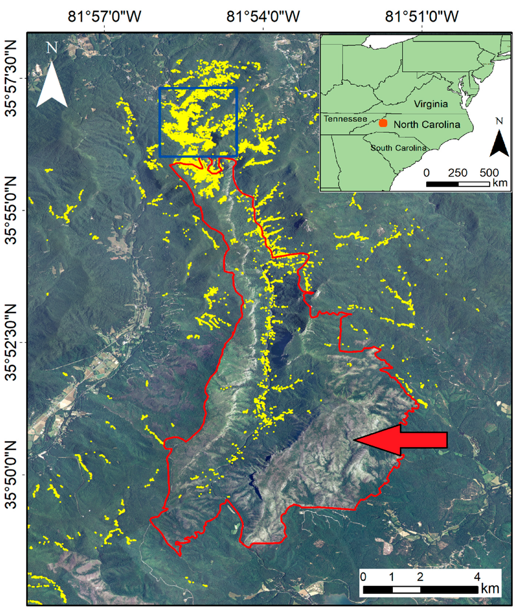
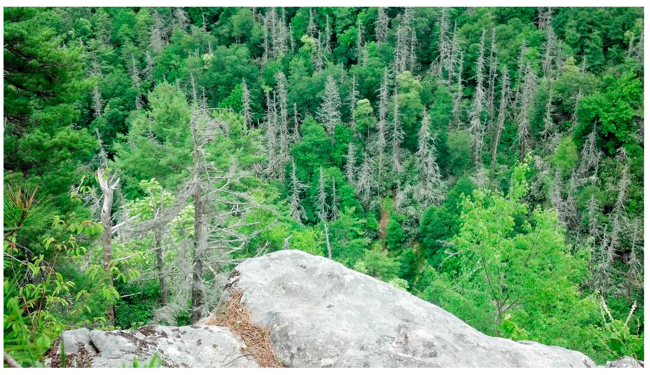
2.1. Study Site

Linville Gorge Wilderness area is located on the eastern edge of the southern Appalachian Mountains in North Carolina, USA (Figure 1). The study area has a rugged terrain with an elevation ranging from 280 to 1300 m. This study focuses on the southern part of this wilderness area of approximately 135 km2. Although the majority of wilderness area remains unlogged [65], two major forest disturbances have occurred since the early 1990s. The first one is HWA infestation in the lower Linville Gorge watershed ([66]; Figure 1), and the second is recurrent wildfires in the southern part of the lower watershed [5,65,66]. Hemlock defoliation in this study site was first reported in the early 2000s [67], and prior to this the defoliation riparian area was dominated by hemlocks in the presence of dense Rhododendron maximum shrubs in the understory [5]. Since the 1950s, this region had not been subjected to large-scale fires until November 2000 [68], when about 4000 ha of the wilderness area was burned by the Brushy Ridge human-initiated fire [5]. Two recent human-initiated fires, “Shortoff and Linville Complex” and “Pinnacle”, were ignited in May 2007 and through June burned about 970 ha and 2000 ha within the gorge area, respectively [5,66]. A large portion of the Pinnacle fire overlapped with the 2000 Brushy Ridge fire [5,66]. Most recently, the White Creek fire burned the same area in March 2017. However, visual interpretation of 10 June 2016, and 3 July 2018, National Agriculture Imagery Program (NAIP) images (with a 1m resolution) showed that this fire was not as extensive as the 2000 and 2007 wildfires.

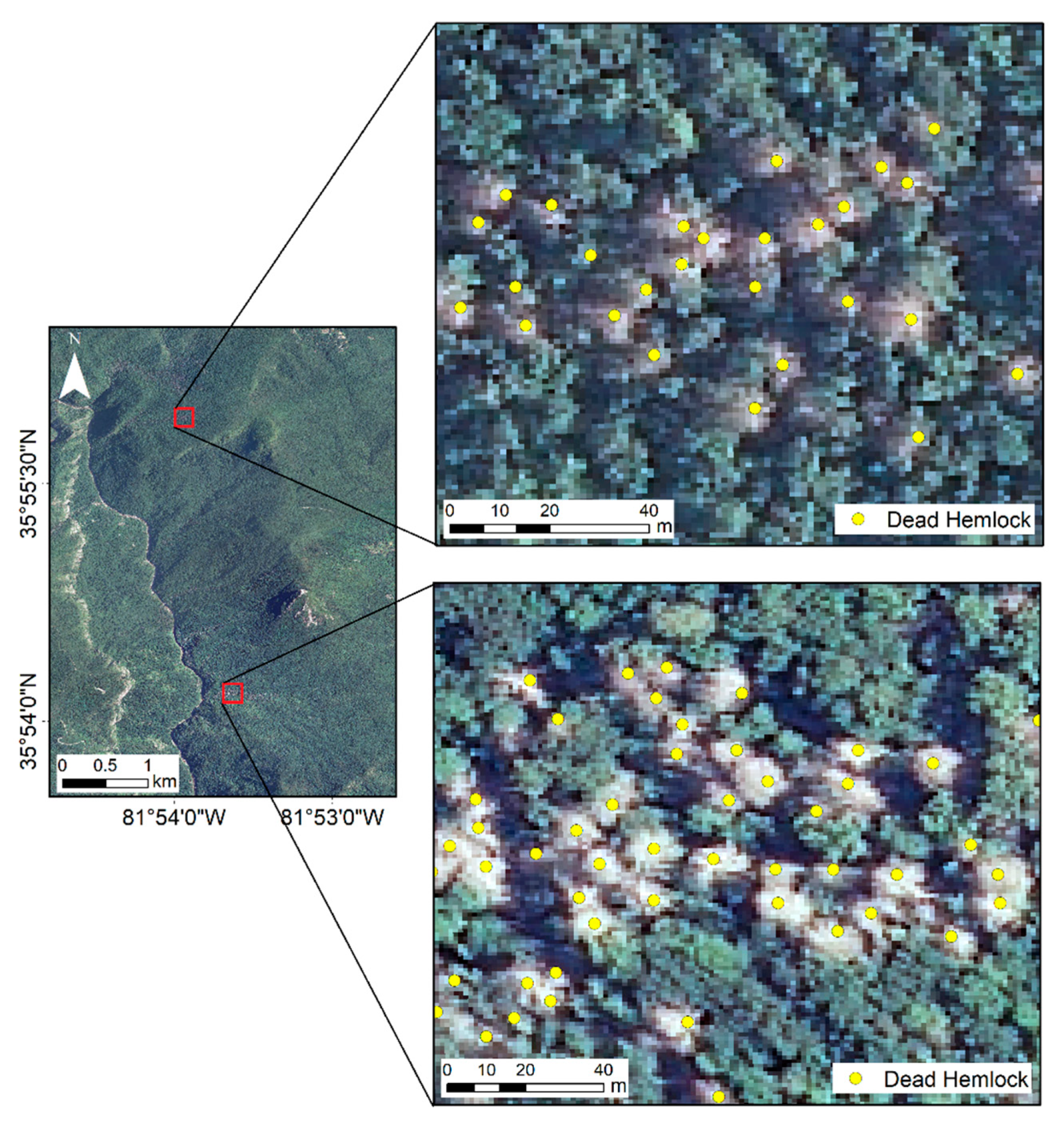
2.2. Digitizing Dead Hemlock Trees

To evaluate and compare the performance of spectral indices in capturing the disturbance intensity, the spatial distribution of the dead hemlocks was used. To delineate the dead hemlock trees, classification methods such as Maximum Likelihood were tested; however, the accuracy of these methods were not as high as expected. Therefore, to build a more accurate map for the validation process of this study, all the dead hemlock trees were visually identified from aerial images. We digitized all the dead or dying conifers exhibiting the white crown and branching structure of hemlocks (Figure 2 and Figure 3) using a high-resolution NAIP image taken on 5 July 2010 (Figure 1). Where there was ambiguity, we also relied on a leaf-off Color-Infrared Digital Orthophoto Quarter Quads (DOQQ) aerial image from 1998 to distinguish the evergreen hemlocks from deciduous trees in these mixed forests. A total of 16,425 dead or dying trees were manually identified and digitized in our study area (Figure 1). Note that this only captured dead overstory trees, and not those in the subcanopy or understory. While all the digitized trees are not likely to be hemlocks, the dead trees conform to known hemlocks’ habitats and observed declines during this period. Ground-based observations give us confidence that the vast majority of the dead trees mapped in this area are hemlocks. We then aggregated these digitized points to the Landsat resolution (30 m) by counting all the digitized dead trees within a single pixel. In this study, the number of dead trees was used as a proxy of hemlock decline intensity at each pixel.

2.3. Landsat Imagery

We downloaded all the available collection-1 level-2 pre-processed Landsat Thematic Mapper (TM) (n = 822) and Operational Land Imager (OLI) (n = 210) scenes from 1990 to 2018 from the USGS Earth Explorer website (https://earthexplorer.usgs.gov/). The surface reflectance products provided by level-2 Landsat TM and Landsat OLI are automatically atmospherically corrected using the Landsat Ecosystem Disturbance Adaptive Processing System (LEDAPS) [69,70] and the Land Surface Reflectance Code (LaSRC) [71] algorithms, respectively. In this study, the Landsat Enhanced Thematic Mapper Plus (ETM+) images were not used due to the gaps caused by Scan Line Corrector (SLC) failure since 2003. We masked out the cloud, cloud shadow, and snow pixels using Matlab scripts and the quality assessment (QA) bands provided by the CFMask algorithm [72,73].

2.4. Temporal Trajectory of Spectral Indices

We integrated frequent Landsat images in statistical analysis and visual interpretation to compare the performance of different spectral indices in (1) determining the temporal dynamics of major disturbances processes, including timing and duration; and (2) capturing the hemlock defoliation intensity, further cross-validated by fine-resolution imagery. We investigated the performance of eight spectral indices—including three TCT indices, two TCT ratio indices, NDVI, Enhanced Vegetation Index (EVI) [74], and DI trajectories (Table 1)—in monitoring the spectral-temporal patterns of forest disturbances. The TCTs were developed by Kauth and Thomas [49] to reduce the dimensionality of spectral data and compress the spectral variation from the original bands into a few principal components [75,76]. We used the first three principal components: brightness (TCB), greenness (TCG), and wetness (TCW). TCB was designed to capture the overall brightness, TCG represents the degree of green vegetation vigor, and TCW shows the variation in the vegetation/soil moisture [52,75,76,77]. The TCT indices of Landsat TM and OLI scenes were calculated using the coefficient provided by Crist et al. [75] and Baig et al. [77], respectively. To reduce the topographic illumination effects of the TCT indices, we also tested the performance of “ratio” indices, such as TCB/TCG (B/G) and TCB/TCW (B/W). The primary topographic effects, changes in solar illumination angle and subsequent surface reflectance, are consistent for all the bands [55,78]; hence, we expected the TCT ratios, NDVI, and EVI to cancel out the topographic effects to some degree [55,79,80,81]. We examined the performance of these eight indices (summarized in Table 1) in highlighting the potential temporal information of disturbance, such as complete tree morbidity, as well as in capturing the hemlock decline intensity. These indices values were rescaled to the [0, 1] range to facilitate the comparison between them.

2.5. Disturbance Detection Algorithm

To estimate the time series model of indices under stable conditions before the disturbances, we separated the study period into pre-disturbance (1990 to 2000) and post-disturbance periods (2001 to 2018). To reduce the influence of outliers, mostly caused by missed clouds, cloud shadows, or snow, the values lower than the 5th or higher than the 95th percentiles were removed from the further analyses. A time series model (Equation (1)), used by Zhu and Woodcock [39] to develop the continuous change detection classification (CCDC) algorithm, was used to separate low-frequency patterns (e.g., long-term patterns or disturbances) from high-frequency signals (e.g., seasonal phenology) at each pixel [39].
p ( t ) i = a i + b i × cos ( 2 π T   t ) + c i × sin ( 2 π T   t ) + d i × t ,
where i is the Landsat pixel number, p(t)i is the predicted index value for the Julian date t of pixel i, t is the Julian date of clear observations in pixel i, and T is the number of days in a year (365). This model has four fitted parameters: a—intercept; b and c—coefficients to model high-frequency signals; and d—first-order coefficient to model low-frequency signal. High-frequency coefficients are designed to capture seasonal phenology or intra-annual changes, while low-frequency coefficients capture long-term linear trends. An iterative nonlinear least squares method was used to fit the time series of the eight spectral indices at each pixel during the pre-infestation period using the Matlab nlinfit function (MathWorks, Natick, MA, USA). The fitted models were then extended to the post-infestation period to calculate the residuals between the observed and modeled values, being used to capture the characteristics of disturbance and recovery at each pixel.

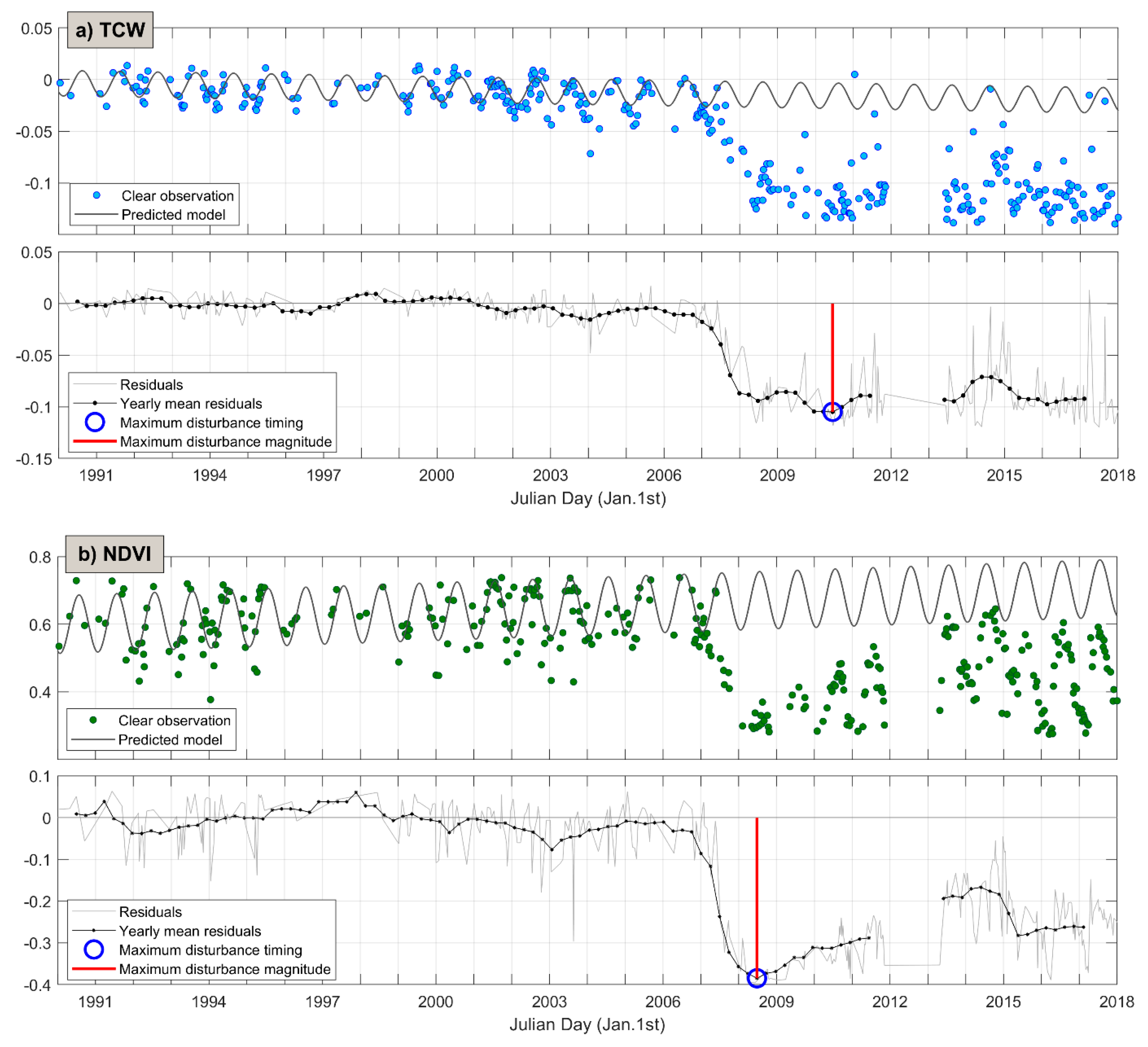
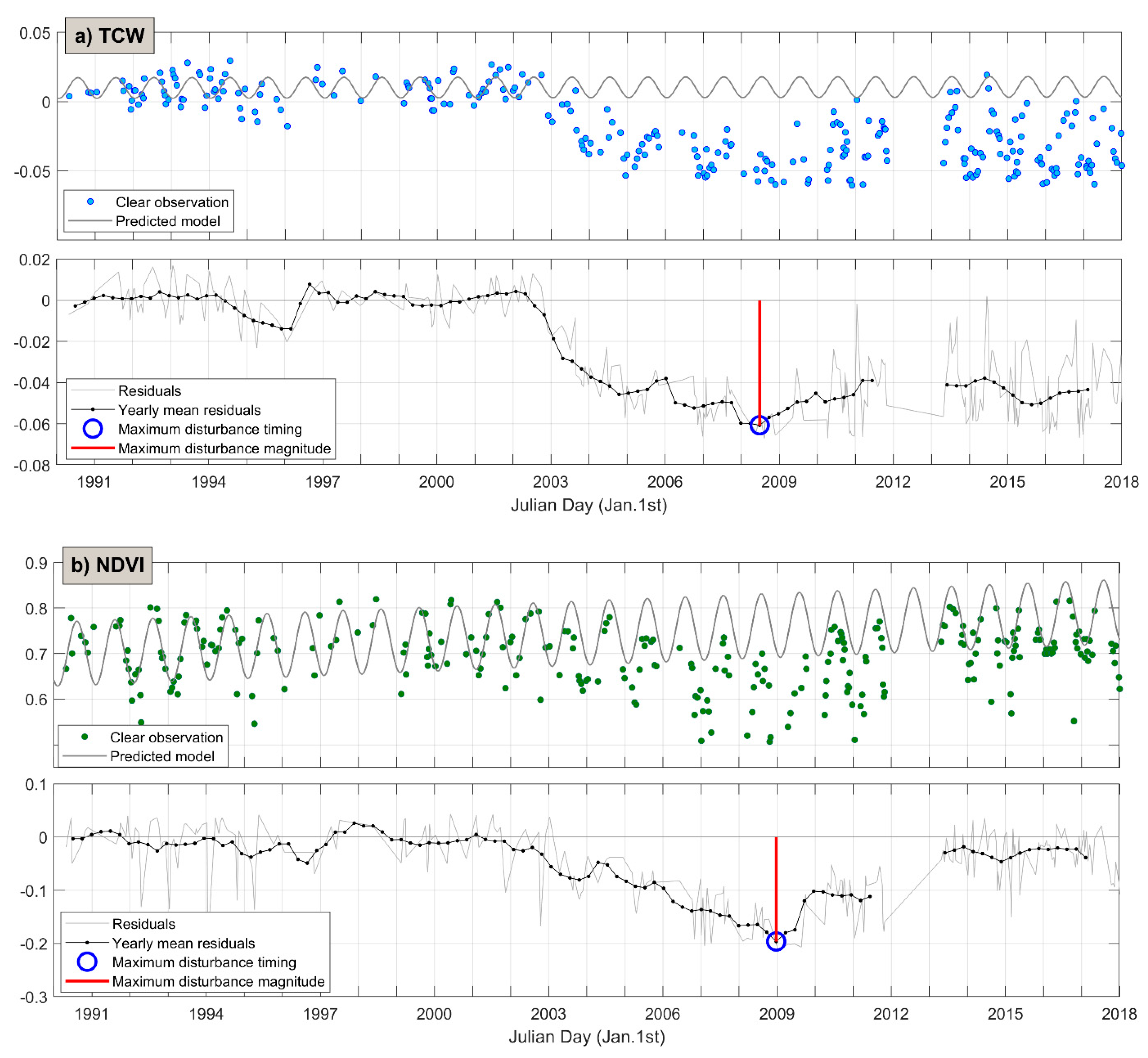
2.6. Maximum Disturbance Timing and Magnitude

For the time series of residual values at each pixel, we applied a moving average method with one-year windows at every three-month time step. This moving average approach was applied (1) to minimize the remnant effects of seasonal variation (e.g., inter-annual variation in phenology) and (2) reduce the effect of outliers and possible short-term changes (e.g., snow or clouds) not filtered by quality control. Note that there is an observational gap between 2012 to 2013 in our Landsat data due to not using the Landsat ETM+ images, so the moving windows overlapping with this gap were not considered in our analysis. From the temporal trajectory of the mean residuals, two metrics were calculated at each pixel: (1) the year with the maximum absolute mean residual as the “maximum disturbance timing”, and (2) the maximum absolute mean residual as the “maximum disturbance magnitude” as an indicator of disturbance intensity. To evaluate if the post-disturbance changes in a pixel are significantly different from the pre-disturbance conditions, a two-sample t-test was used. The t-test was applied to the residuals of the pre-disturbance period and the residuals within the 1-year window with the maximum absolute mean residual. Pixels with no significant changes from the pre-disturbance conditions were excluded for the further analysis.
Two sub-regions were selected for further evaluation. Sub-region 1, with a 5.7 km2 forested area (80 × 80 Landsat pixels) including both HWA defoliated pixels and non-defoliated pixels, was selected to investigate the capability of the indices in capturing the infestation timing and intensity (Figure 1). No wildfire has been reported in this sub-region. Sub-region 2 with a 47.5 km2 area was located in the southern Linville Gorge Wilderness area where most wildfires occurred (Figure 1). To compare the performance of our metrics in capturing the fire disturbance timing, we also used the Linville Gorge fire history map between 1980 and 2017, which has been mapped by the Wildland Fire Decision Support System (WFDSS) (https://wfdss.usgs.gov). We compare the maximum disturbance timing maps from the eight spectral indices in terms of the perimeters of fire and occurrence year of this map.
To evaluate the hemlock decline intensity estimated from the eight spectral indices, we compared the maximum disturbance magnitude maps with the number of dead hemlocks per pixel (as a representative of decline intensity) and their spatial distribution. To compare the indices’ performances, the maximum disturbance magnitude maps of sub-region 1 with different dynamic ranges were rescaled using the maximum and minimum values. To evaluate the performance of the indices, we first produced boxplots of the scaled maximum disturbance magnitudes grouped by the number of dead hemlocks. Then, a linear regression analysis was applied between the number of dead hemlocks and the median maximum disturbance magnitude values of pixels with the same number of dead hemlocks. Due to the small sample size, we grouped the pixels with 10 or more dead hemlocks into one group.

3. Results

3.1. Temporal Dynamics of Indices Time Series

First, we show examples that give the spectral trajectories of TCW and NDVI in two Landsat pixels: (1) a pixel with a fire occurrence in 2007 (Figure 4) and (2) an HWA-defoliated pixel with 12 dead hemlocks without fire (Figure 5). The fire in 2007 was characterized as an abrupt change in the TCW (Figure 4a), NDVI (Figure 4b), EVI (Figure S1c), and B/G (Figure S1d). The hemlock decline, however, was captured as more a gradual change in all the indices for the selected pixels (Figure 5 and Figure S2). Compared to the other indices, the TCB time-series is noisy with more inconsistent seasonal patterns (Figures S1a and S2a). TCB slightly increased during the disturbances (Figures S1a and S2a) because disturbed pixels might have a higher background reflectance than undisturbed ones. TCG, TCW, NDVI, and EVI values, on the other hand, decreased due to defoliation, corresponding dryness, and background color changes (Figure 4 and Figure 5, Figures S1 and S2). Subsequently, the B/G and DI values increased with forest disturbances (Figures S1 and S2), while the B/W values decreased (Figures S1e and S2e). TCW (Figure 4a and Figure 5a) had a smaller intra-annual variability during the pre-disturbance period than the other indices.
Pixel-based observations indicate that the spectral trajectories of these indices have the potential to provide temporal information regarding disturbance onset, maximum disturbance timing, and subsequent sub-canopy recovery (Figure 4 and Figure 5, Figures S1 and S2). The temporal patterns of the HWA-defoliated pixel showed that the gradual declines of TCG, TCW, NDVI, and EVI, as well as gradual increases of TCB, B/G, and DI began around 2003, and maximum forest disturbance occurred between 2007 and 2010 (Figure 5 and Figure S2). This suggests that it took about 4 to 7 years for the initial HWA outbreak to complete hemlock mortality.
The maximum disturbance timing maps are shown for sub-region 1 (Figure 6) and sub-region 2 (Figure 7). NDVI, B/G, and TCG detected the maximum disturbance timing more accurately and consistently than the other indices, while TCB and B/W showed the weakest performance. Based on TCB and B/W, the maximum disturbance for most of the pixels in sub-region 1 occurred before 2006, which is unlikely to be based on the hemlock decline initial timing and duration of HWA defoliation [12,18,67]. Our result showed that in the maximum disturbance timing maps of NDVI and B/G, 66.24% and 62.35% pixels of the 2007 fire boundary were accurately captured as 2007 or 2008, respectively. TCG, EVI, TCW, and DI also captured about 57.1%, 54.2%, 38.2%, and 23.85% of the pixels of the 2007 fire boundary as 2007 or 2008, respectively. For most of HWA-defoliated pixels, the maximum disturbance timing suggested by TCW was either 2008, 2009, or 2010, while those years identified by NDVI, B/G, and TCG are mostly 2007 (Figure 6).
The disturbance timing maps of sub-region 2 from TCG, TCW, NDVI, EVI, B/G, and DI generally agree well with the WFDSS fire history map (Figure 7). The NDVI-derived disturbance timing was slightly more accurate than the other indices (Figure 7e), where it captured the 2007 fire as the same year and the 2000 fire with about a one-year delay. Although B/G, TCG, EVI, and TCW captured the fire timing relatively well (especially the May 2007 fire), they showed slightly lagged responses in some areas. The timing maps from these four indices indicated that the 2007 fire was detected as either 2007 or 2008, and the November 2000 fire was captured between 2000 and 2002 (Figure 7). The overall performance of the brightness-related indices (TCB, B/W, and DI) in detecting this timing for pixels with a wildfire history was lower than that of the other metrics (Figure 7).

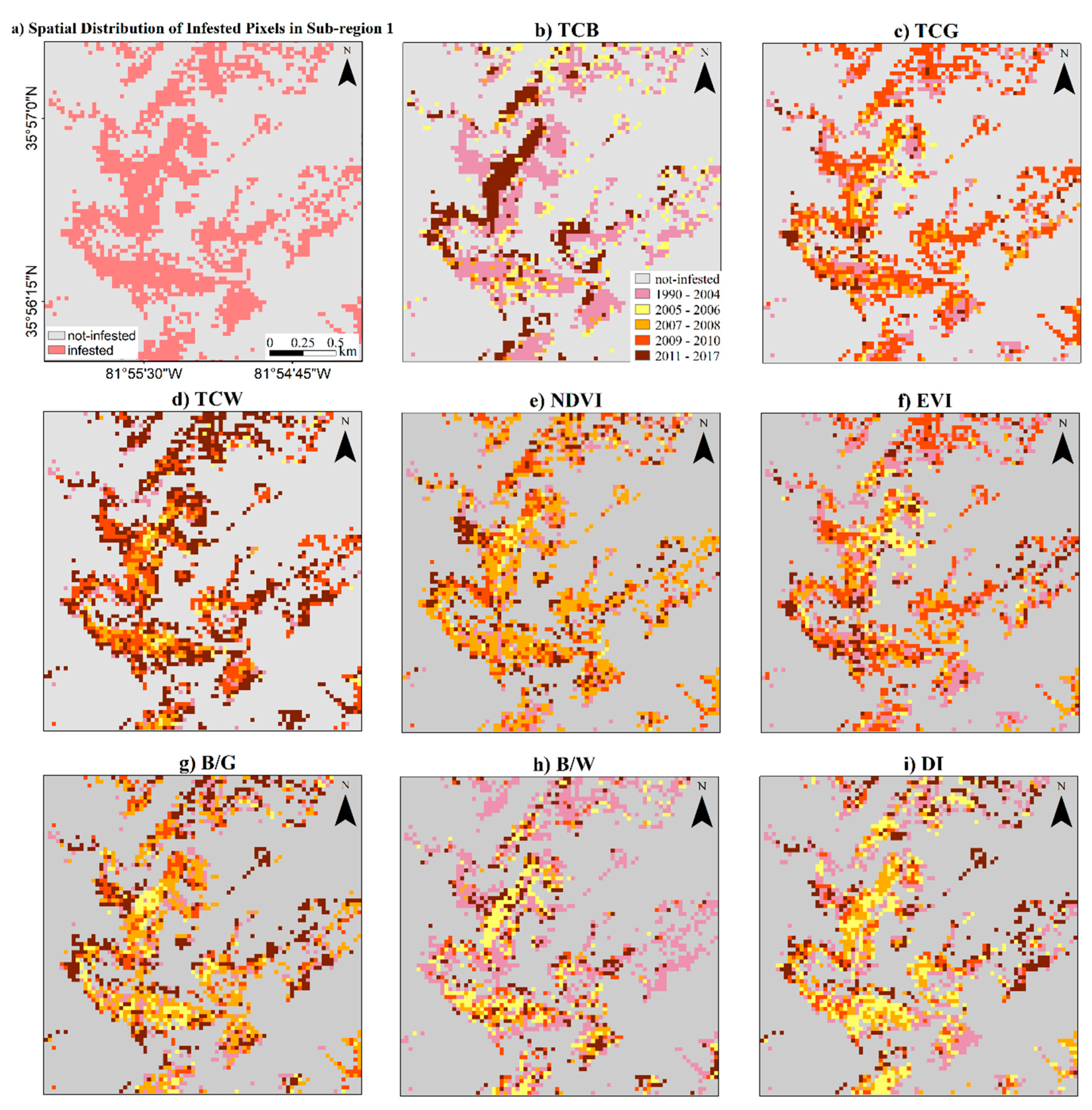
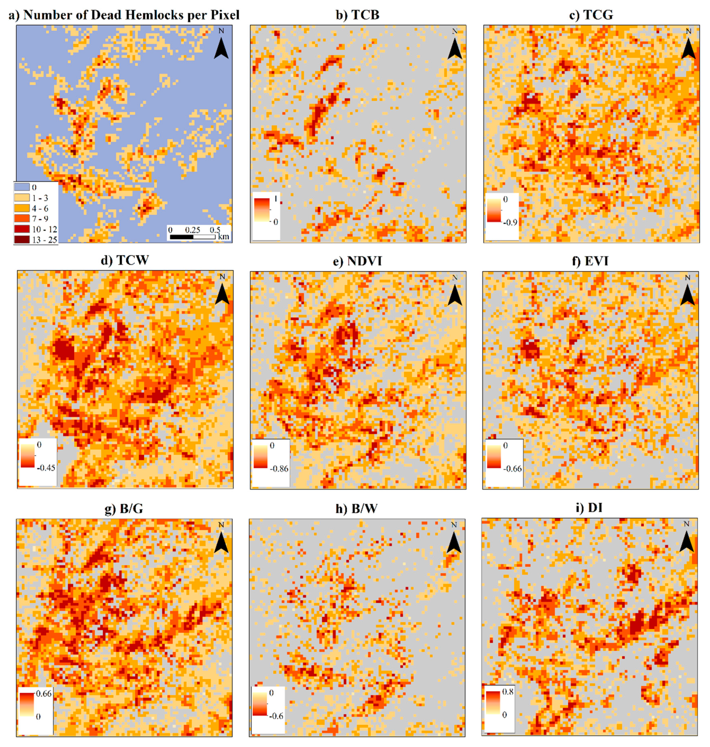
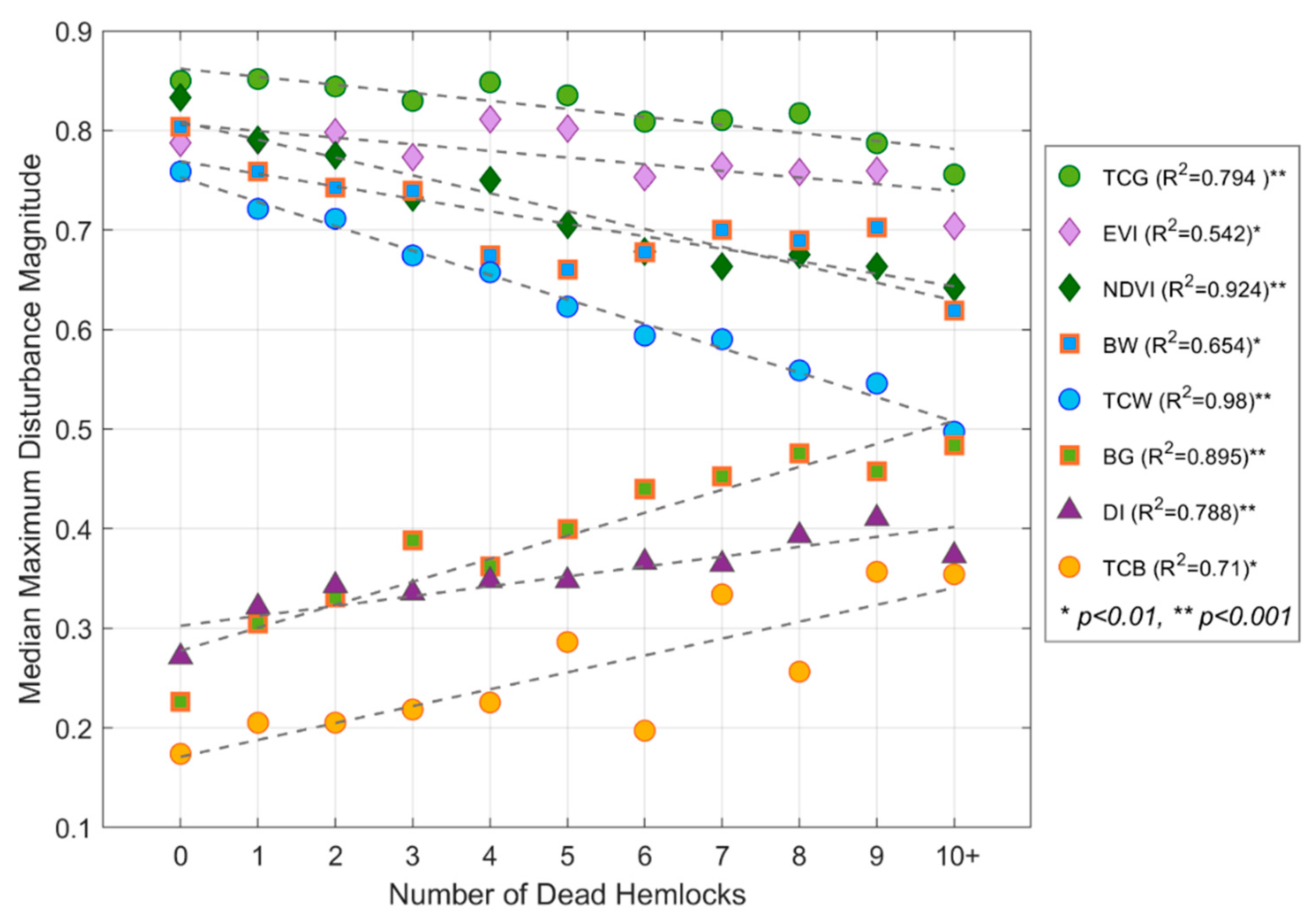
3.2. Hemlocks Decline Intensity and Maximum Disturbance Magnitude

Comparisons of the maximum disturbance magnitude maps with the number of dead hemlocks within sub-region 1 also demonstrate that TCW and NDVI were more in agreement with the dead hemlock distribution than the other metrics (Figure 8). The TCB, TCG, EVI, B/G, B/W, and DI maximum disturbance magnitude maps, on the other hand, did not match with the infestation intensity as well as TCW and NDVI (Figure 8). For each index, the median maximum disturbance magnitudes for pixels with the same number of dead hemlocks were extracted from the metrics’ boxplots (Figure S3) and entered into the linear regression analysis. The relationships were statistically significant for all the indices (p < 0.01), although the accuracy varied (Figure 9). TCW and NDVI were the best predictors of the hemlock decline intensity (R2 = 0.98 and 0.924, respectively; Figure 9), while TCB, EVI, and B/W showed the weakest performances.

4. Discussion

In this study, all the available Landsat images were used to explore the capability of eight spectral indices to characterize the spectral-temporal dynamics of the forest fire and infestation disturbances. Our results indicate that dense time series Landsat images enabled us to detect both the timing and intensity of the disturbances accurately. Pixel-based interpretation showed that all eight indices were able to capture the changes associated with the forest disturbances; however, their accuracy in highlighting the characteristics varied. TCB had an inconsistent seasonal cycle, and the spectral differences represented some extreme unexpected values (Figures S1a and S2a), which produced the weakest overall performance in characterizing disturbances. The inconsistent patterns of TCB and TCG are likely attributed to the sensitivity of these indices to the complex terrain [55] and the different sun angles of images with different acquisition dates [82]. Based on pixel-based visualization, the detected timing for TCB and B/G can be also explained by its post-disturbance pattern, where the TCB values during recovery stage are as high as the disturbance period (Figures S1a and S2a). TCW also showed a smaller seasonal variability compared to TCB during the pre-disturbance period, which is also reported by another study [56]. Increasing or decreasing the pattern of the spectral indices during the disturbances corresponded well with other studies [15,42,50,75].

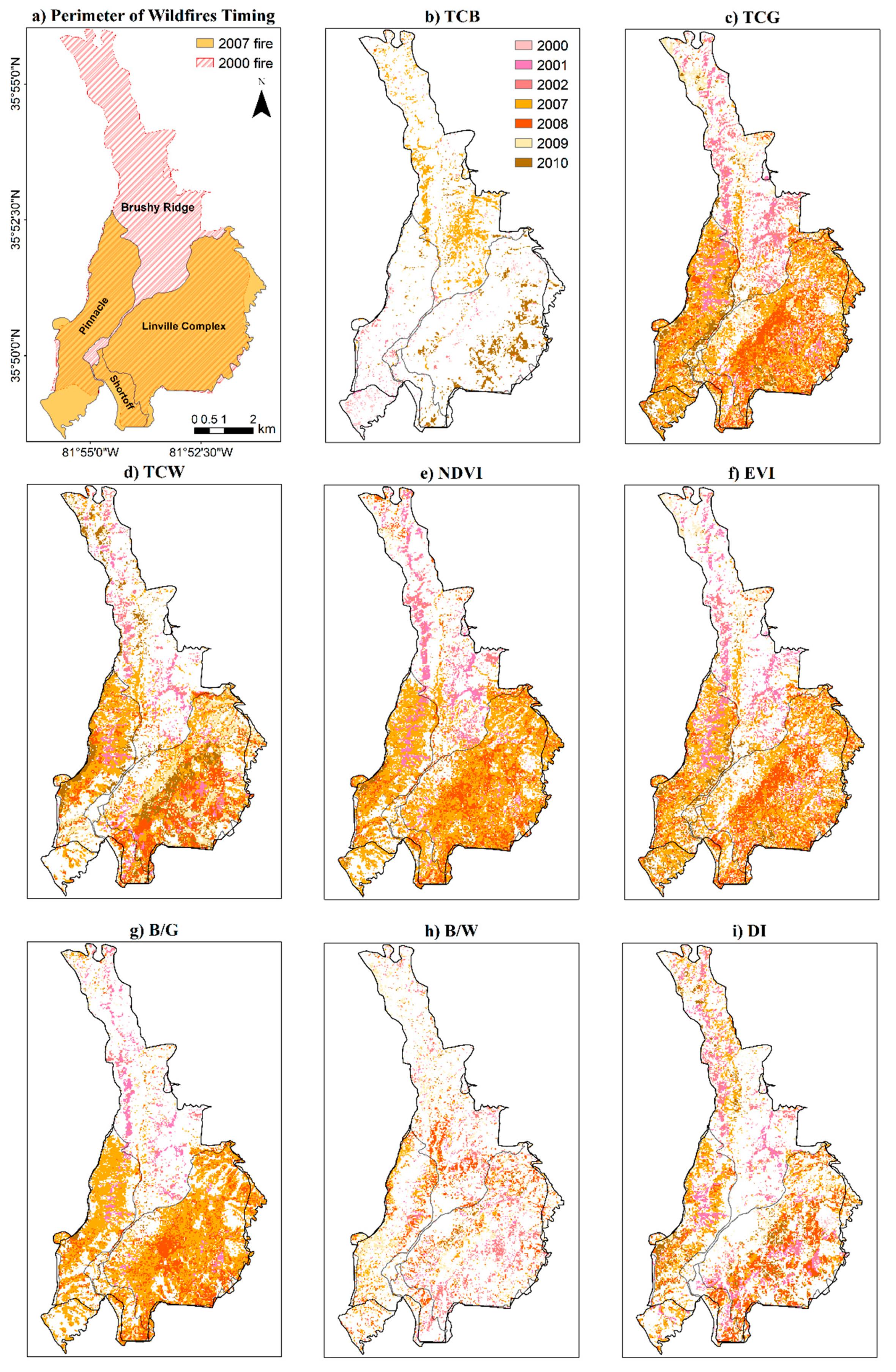
4.1. Maximum Disturbance Timing

The initial timing of hemlock declines from the visual interpretation of trajectories aligns with other studies, where the outbreak of HWA in North Carolina was reported in early 2000s [10,67]. TCW and NDVI, followed by TCG, B/G, EVI, and DI, have the most consistent performance in identifying the maximum disturbance timing for infestation (Figure 6). The maximum disturbance timing estimated by the spectral indices suggests that HWA takes about 4 to 7 years to complete stand mortality. This is in agreement with other studies in this region, which documented 4–6 years for complete hemlocks mortality [12,18]. For example, Ford et al. [10] reported that 6 years after the initial outbreak of HWA in the southern Appalachian, more than 80% of the hemlocks were completely dead. B/G, TCG, and EVI performed well in detecting the maximum disturbance timing for fire (Figure 7), which is in agreement with other studies [83,84] and may suggest that these indices perform better in characterizing abrupt disturbances.
TCW identified the maximum disturbance timing with 1-year or more lags consistently for both the infestation and fire, compared to NDVI (Figure 6 and Figure 7). NDVI captured both the hemlocks’ decline and fire disturbance timing more accurately than the other indices (Figure 6 and Figure 7). A possible explanation could be the ability of NDVI to detect changes in vegetation density during the recovery period. Based on the pixel-level observations of the TCW trajectory, no clear recovery was observed (Figure 4 and Figure 5). The lagged detection of the maximum disturbance timing was likely the result of TCW producing large negative values (Figure 4 and Figure 5) even after the subcanopy recovery verified in field observations (Figure 2). The negative residuals and increased seasonal amplitudes in TCW during the recovery influenced the mean residuals and produced the delayed maximum disturbance timing, while NDVI showed steep increasing patterns at the initial stage of recovery. Another explanation for the delayed responses of all indices for the 2000 fire event (Figure 7) may be because this fire occurred late in the year (November); hence, in our moving average approach the maximum absolute mean residuals could happen with at least a one-year delay (Figure 7). In addition, our analysis did not detect the 2000 timing for many pixels within the perimeter, which might be explained by the fact that the WFDSS map includes many lightly burned or even unburned areas. For example, the 2010 NAIP image still showed that some hemlocks stands within the 2000 fire perimeter from the WFDSS map, and it was very likely that the fire in 2000 lightly burned the study area.

4.2. Maximum Disturbance Magnitude

Although TCG was a good indicator of disturbance timing for both the infestation and fire (Figure 6c and Figure 7c), it was not a good predictor of the hemlock decline intensity (Figure 8c). It was likely that the biased values in the TCG trajectory affected the maximum disturbance magnitudes. Both the B/G and B/W ratios, designed to minimize the possible topographic effects, performed better than TCB in capturing the disturbance timing and magnitude. However, these ratio indices were sensitive to extremely small values in the denominator, and therefore produced quite unstable time series. Although the maximum disturbance timing maps derived from B/G were reliable (Figure 6g and Figure 7g), the maximum disturbance magnitude did not match well with the number of dead hemlocks (Figure 8g). The Disturbance Index (DI), introduced to accentuate the difference between the disturbed and undisturbed forest conditions [42,85], did not perform better than TCW and NDVI in detecting the maximum disturbance timing and hemlock decline intensity (Figure 6i, Figure 7i and Figure 8i). The better performance of DI in detecting infestation intensity, compared to TCB and TCG, might be explained by the usage of the normalized TCT values in its calculation, which would minimize the effects of seasonality and variability due to bidirectional reflectance [85,86].
The maximum disturbance magnitudes of TCW and NDVI were relatively comparable with the spatial distribution of the dead hemlock trees (Figure 8). In all the disturbance magnitude maps (Figure 8), some pixels with no digitized dead hemlocks had large absolute disturbance magnitudes, while some severely infested pixels had small absolute disturbance magnitudes. These unexpected results might be explained in a few ways. First, the complex rugged terrain of the study area can limit the performance of spectral indices, especially the ones that are more sensitive to topography variation, such as TCB and TCG [55,87], leading to biased high or low relative residuals and inaccurate estimates. Song and Woodcock [55] also reported that while TCB and TCG were sensitive to topographic effects especially when the solar zenith angle was large, TCW and NDVI are less sensitive. While DI could minimize the topographic effect by using normalized TCT, it can still be affected by topography, inherited from the TCB and TCG variability. Studies also reported that although EVI can reduce the effects of atmospheric conditions and vegetation saturation, compared to NDVI it is sensitive to topographic and viewing illumination effects due to the presence of the soil adjustment factor in its equation [80,88,89,90]. Second, there could be uncertainty in identifying the hemlock decline intensity at each pixel based on the number of dead hemlocks. HWA kills hemlocks across all ages and sizes eventually [7], but their progresses are different based on their sizes [25]. Therefore, the number of overstory dead hemlocks, as a proxy of hemlock decline intensity, without considering the projected crown sizes, overlapping, and possible understory dead hemlocks, may either underestimate or overestimate the infestation intensity within a single pixel, not even mentioning geometric errors. Third, requiring clear remote sensing observations can produce small sample sizes in pixels with persistent clouds or cloud shadows, thereby undermining the reliability and robustness of parameter estimates in our regression models [39].

4.3. Post-Infestation Recovery

Another important information that can be retrieved is the recovery progress after the disturbances. For example, the spectral trajectories of two example pixels (Figure 4 and Figure 5, Figures S1 and S2) indicated that all indices, except TCB and B/W, indicated onsets of recovery after 7–8 years of the initial infestation (Figure 5), which also showed the stable seasonal patterns around 2014. While TCW reliably identified the timing and magnitude of the disturbance, it has limitations in determining the potential post-infestation recovery. The TCW residuals decreased toward negative values during the entire period of infestation and recovery, and they never recovered, especially during the dormancy seasons, to the pre-infestation level (Figure 5). The current evergreen hemlocks stands are being replaced by deciduous trees, such as black birch (Betula lenta L.) and maple (Acer spp.) (Figure 2) [91]. Emerging leaf-off periods during this transition from evergreen to deciduous trees might indicate that TCW might have limitations in detecting forest decline and following recoveries using image difference [15]. Overall, our time series analysis also suggested that the seasonal dynamic of some indices could be appropriate to characterize forest recovery following the disturbances. However, such indices should be chosen more carefully, and the interpretation of the recovery patterns should depend on subsequent species replacement. Future studies might be needed to validate the results with ground-based observations in terms of recovery patterns.

4.4. Limitations of the Developed Method

Our method has some limitations. First, to fit the time series model during an undisturbed period, it is necessary to have detailed historical information of the study area, such as the fire history and perimeter, as well as high-resolution aerial photos. Therefore, in a region with frequent disturbances, such as wildfires, defining a pre-disturbance period can be challenging. Second, in this study to evaluate the performance of the indices we developed our algorithm to focus only on the maximum disturbance events over the period of recording. However, it should be noted that this method could be adapted to identify (local) maxima when the analysis of multiple disturbances is of interest. Our analysis on pixels with both the 2000 and 2007 fires in the study site (Figure S4) showed that our approach could be modified to detect multiple disturbances if we were to dig into several disturbance timings.

5. Conclusions

In this study, we examined the capability of eight spectral indices to capture the spectral and temporal dynamics of fire and infestation disturbances in the southern Appalachian forest using all available Landsat images. We estimated these disturbance characteristics in space and time based on the residuals between the observed and predicted values of multi-frequency remote sensing data, separating the inter-annual disturbance patterns (low frequency) and seasonal phenology (high frequency) signals. In addition, we investigated the performance of these indices in capturing the hemlock decline intensity, validated with the number of dead trees identified at each pixel. Our results suggested that NDVI, followed by TCW, showed the most reliable performance in detecting the temporal-spectral properties of forest disturbances in complex terrain, while TCB, B/W, and EVI have the poorest performance in characterizing disturbances. Although TCW showed relatively consistent results in capturing the disturbance regimes, it might have limitations in detecting recovery patterns. Our study highlights the value of using long-term Landsat imagery to monitor forest conditions over space and time for forest disturbances and recovery.

Supplementary Materials

The following are available online at https://www.mdpi.com/2072-4292/12/15/2412/s1, Figure S1: The spectral trajectory of TCB, TCG, EVI, B/G, B/W, and DI; their residuals; and the mean values within 1-year moving windows with 3-month steps at a Landsat pixel with a fire in 2007. Figure S2: The spectral trajectory of TCB, TCG, EVI, B/G, B/W, and DI; their residuals; and the mean values within 1-year moving windows with 3-month steps at a Landsat pixel with 12 dead hemlocks. Figure S3: Boxplots of indices’ maximum disturbance magnitude as a function of the number of dead hemlocks in a pixel. Figure S4: The spectral trajectories of NDVI for a Landsat pixel with both 2000 and 2007 fires.

Author Contributions

Conceptualization, M.K. and T.H.; methodology, M.K., T.H. and S.M.R.; software, M.K. and J.K.; validation, M.K. and S.P.N.; formal analysis, M.K., T.H., S.M.R. and C.S.; investigation, M.K.; resources, M.K., and S.P.N.; data curation, M.K., J.K. and S.P.N.; writing—original draft preparation, M.K.; writing—review and editing, M.K., T.H., C.S., S.P.N., S.M.R., and J.K.; visualization, M.K.; supervision, T.H.; project administration, T.H.; funding acquisition, T.H. All authors have read and agreed to the published version of the manuscript.

Funding

This research was supported by the NASA Carbon Science program (Grant # NNX17AE69G) to T Hwang and C Song, and the National Science Foundation (NSF) Long Term Ecological Research (LTER) Program award to the Coweeta LTER (Grant # DEB-0823293).

Acknowledgments

We wish to thank Sara Thompson for helping us in the process of data collecting.

Conflicts of Interest

The authors declare no conflict of interest. Any opinions, findings, conclusions, or recommendations expressed in the material are those of the authors and do not necessarily reflect the views of NASA or NSF.

References

  1. Masek, J.G.; Goward, S.N.; Kennedy, R.E.; Cohen, W.B.; Moisen, G.G.; Schleeweis, K.; Huang, C. United States forest disturbance trends observed using Landsat time series. Ecosystems 2013, 16, 1087–1104. [Google Scholar] [CrossRef] [Green Version]
  2. van Lierop, P.; Lindquist, E.; Sathyapala, S.; Franceschini, G. Global forest area disturbance from fire, insect pests, diseases and severe weather events. For. Ecol. Manag. 2015, 352, 78–88. [Google Scholar] [CrossRef] [Green Version]
  3. Lovett, G.M.; Canham, C.D.; Arthur, M.A.; Weathers, K.C.; Fitzhugh, R.D. Forest ecosystem responses to exotic pests and pathogens in eastern North America. BioScience 2006, 56, 395–405. [Google Scholar] [CrossRef] [Green Version]
  4. Waldron, J.D.; Lafon, C.W.; Coulson, R.N.; Cairns, D.M.; Tchakerian, M.D.; Birt, A.; Klepzig, K.D. Simulating the impacts of southern pine beetle and fire on the dynamics of xerophytic pine landscapes in the southern Appalachians. Appl. Veg. Sci. 2007, 10, 53–64. [Google Scholar] [CrossRef]
  5. Wimberly, M.C.; Reilly, M.J. Assessment of fire severity and species diversity in the southern Appalachians using Landsat TM and ETM+ imagery. Remote Sens. Environ. 2007, 108, 189–197. [Google Scholar] [CrossRef] [Green Version]
  6. Ellison, A.M.; Bank, M.S.; Clinton, B.D.; Colburn, E.A.; Elliott, K.; Ford, C.R.; Foster, D.R.; Kloeppel, B.D.; Knoepp, J.D.; Lovett, G.M. Loss of foundation species: Consequences for the structure and dynamics of forested ecosystems. Front. Ecol. Environ. 2005, 3, 479–486. [Google Scholar] [CrossRef]
  7. Vose, J.M.; Wear, D.N.; Mayfield, A.E.; Nelson, C.D. Hemlock woolly adelgid in the southern Appalachians: Control strategies, ecological impacts, and potential management responses. For. Ecol. Manag. 2013, 291, 209–219. [Google Scholar] [CrossRef]
  8. Pacala, S.W.; Canham, C.D.; Silander, J., Jr. Forest models defined by field measurements: I. The design of a northeastern forest simulator. Can. J. For. Res. 1993, 23, 1980–1988. [Google Scholar] [CrossRef]
  9. Kantola, T.; Lyytikäinen-Saarenmaa, P.; Coulson, R.N.; Strauch, S.; Tchakerian, M.D.; Holopainen, M.; Saarenmaa, H.; Streett, D.A. Spatial distribution of hemlock woolly adelgid induced hemlock mortality in the Southern Appalachians. Open J. For. 2014, 4, 492. [Google Scholar] [CrossRef] [Green Version]
  10. Ford, C.R.; Elliott, K.J.; Clinton, B.D.; Kloeppel, B.D.; Vose, J.M. Forest dynamics following eastern hemlock mortality in the southern Appalachians. Oikos 2012, 121, 523–536. [Google Scholar] [CrossRef] [Green Version]
  11. Webster, J.; Morkeski, K.; Wojculewski, C.; Niederlehner, B.; Benfield, E.; Elliott, K. Effects of hemlock mortality on streams in the southern Appalachian Mountains. Am. Midl. Nat. 2012, 168, 112–132. [Google Scholar] [CrossRef]
  12. McClure, M.S. Density-dependent feedback and population cycles in Adelges tsugae (Homoptera: Adelgidae) on Tsuga canadensis. Environ. Entomol. 1991, 20, 258–264. [Google Scholar] [CrossRef]
  13. Orwig, D.A.; Foster, D.R.; Mausel, D.L. Landscape patterns of hemlock decline in New England due to the introduced hemlock woolly adelgid. J. Biogeogr. 2002, 29, 1475–1487. [Google Scholar] [CrossRef] [Green Version]
  14. Stoetzel, M.B.; Onken, B.; Reardon, R.; Lashomb, J. History of the introduction of Adelges tsugae based on voucher specimens in the Smithsonian Institute National Collection of Insects. In Proceedings of the Hemlock Woolly Adelgid in the Eastern United States Symposium, East Brunswick, NJ, USA, 5–7 February 2002. [Google Scholar]
  15. Jones, C.; Song, C.; Moody, A. Where’s woolly? An integrative use of remote sensing to improve predictions of the spatial distribution of an invasive forest pest the Hemlock Woolly Adelgid. For. Ecol. Manag. 2015, 358, 222–229. [Google Scholar] [CrossRef]
  16. Krapfl, K.J.; Holzmueller, E.J.; Jenkins, M.A. Early impacts of hemlock woolly adelgid in Tsuga canadensis forest communities of the southern Appalachian Mountains1. J. Torrey Bot. Soc. 2011, 138, 93–107. [Google Scholar] [CrossRef]
  17. Kizlinski, M.L.; Orwig, D.A.; Cobb, R.C.; Foster, D.R. Direct and indirect ecosystem consequences of an invasive pest on forests dominated by eastern hemlock. J. Biogeogr. 2002, 29, 1489–1503. [Google Scholar] [CrossRef]
  18. Eschtruth, A.K.; Cleavitt, N.L.; Battles, J.J.; Evans, R.A.; Fahey, T.J. Vegetation dynamics in declining eastern hemlock stands: 9 years of forest response to hemlock woolly adelgid infestation. Can. J. For. Res. 2006, 36, 1435–1450. [Google Scholar] [CrossRef]
  19. Pontius, J.; Hallett, R.; Martin, M. Using AVIRIS to assess hemlock abundance and early decline in the Catskills, New York. Remote Sens. Environ. 2005, 97, 163–173. [Google Scholar] [CrossRef]
  20. Nowacki, G.J.; Abrams, M.D.J.B. The demise of fire and “mesophication” of forests in the eastern United States. BioScience 2008, 58, 123–138. [Google Scholar] [CrossRef]
  21. Abrams, M.D.; Nowacki, G.J. Exploring the early Anthropocene burning hypothesis and climate-fire anomalies for the eastern US. J. Sustain. For. 2015, 34, 30–48. [Google Scholar]
  22. Abrams, M.D. Where has all the white oak gone? BioScience 2003, 53, 927–939. [Google Scholar] [CrossRef] [Green Version]
  23. McEwan, R.W.; Dyer, J.M.; Pederson, N.J.E. Multiple interacting ecosystem drivers: Toward an encompassing hypothesis of oak forest dynamics across eastern North America. Ecography 2011, 34, 244–256. [Google Scholar] [CrossRef]
  24. Yorks, T.E.; Jenkins, J.C.; Leopold, D.J.; Raynal, D.J.; Orwig, D.A. Influences of Eastern Hemlock Mortality on Nutrient Cycling; McManus, K.A., Shields, K.S., Souto, D.R., Souto, D.R., Eds.; U.S. Department of Agriculture, Forest Service, Northeastern Forest Experiment Station: Newtown Square, PA, USA, 2000; pp. 126–133. [Google Scholar]
  25. Kim, J.; Hwang, T.; Schaaf, C.L.; Orwig, D.A.; Boose, E.; Munger, J.W. Increased water yield due to the hemlock woolly adelgid infestation in New England. Geophys. Res. Lett. 2017, 44, 2327–2335. [Google Scholar] [CrossRef]
  26. Brantley, S.; Ford, C.R.; Vose, J.M. Future species composition will affect forest water use after loss of eastern hemlock from southern Appalachian forests. Ecol. Appl. 2013, 23, 777–790. [Google Scholar] [CrossRef] [PubMed]
  27. Royle, D.; Lathrop, R. Discriminating Tsuga canadensis hemlock forest defoliation using remotely sensed change detection. J. Nematol. 2002, 34, 213. [Google Scholar] [PubMed]
  28. Kantola, T.; Lyytikainen-Saarenmaa, P.; Coulson, R.N.; Holopainen, M.; Tchakerian, M.D.; Streett, D.A. Development of monitoring methods for Hemlock Woolly Adelgid induced tree mortality within a Southern Appalachian landscape with inhibited access. IForest 2016, 9, 178–186. [Google Scholar] [CrossRef] [Green Version]
  29. Bradley, B.A. Remote detection of invasive plants: A review of spectral, textural and phenological approaches. Biol. Invasions 2014, 16, 1411–1425. [Google Scholar] [CrossRef]
  30. Diao, C.; Wang, L. Incorporating plant phenological trajectory in exotic saltcedar detection with monthly time series of Landsat imagery. Remote Sens. Environ. 2016, 182, 60–71. [Google Scholar] [CrossRef]
  31. Song, C.; Chen, J.M.; Hwang, T.; Gonsamo, A.; Croft, H.; Zhang, Q.; Dannenberg, M.; Zhang, Y.; Hakkenberg, C.; Li, J. Ecological characterization of vegetation using multisensor remote sensing in the solar reflective spectrum. Remote Sens. Handb. 2015, 2, 533–575. [Google Scholar]
  32. Hermosilla, T.; Wulder, M.A.; White, J.C.; Coops, N.C.; Hobart, G.W. Regional detection, characterization, and attribution of annual forest change from 1984 to 2012 using Landsat-derived time-series metrics. Remote Sens. Environ. 2015, 170, 121–132. [Google Scholar] [CrossRef]
  33. Wulder, M.A.; White, J.C.; Goward, S.N.; Masek, J.G.; Irons, J.R.; Herold, M.; Cohen, W.B.; Loveland, T.R.; Woodcock, C.E. Landsat continuity: Issues and opportunities for land cover monitoring. Remote Sens. Environ. 2008, 112, 955–969. [Google Scholar] [CrossRef]
  34. Huang, C.; Goward, S.N.; Masek, J.G.; Thomas, N.; Zhu, Z.; Vogelmann, J.E. An automated approach for reconstructing recent forest disturbance history using dense Landsat time series stacks. Remote Sens. Environ. 2010, 114, 183–198. [Google Scholar] [CrossRef]
  35. Cohen, W.B.; Goward, S.N. Landsat’s role in ecological applications of remote sensing. Bioscience 2004, 54, 535–545. [Google Scholar] [CrossRef]
  36. Kennedy, R.E.; Yang, Z.; Cohen, W.B. Detecting trends in forest disturbance and recovery using yearly Landsat time series: 1. LandTrendr—Temporal segmentation algorithms. Remote Sens. Environ. 2010, 114, 2897–2910. [Google Scholar] [CrossRef]
  37. Schultz, M.; Verbesselt, J.; Avitabile, V.; Souza, C.; Herold, M. Error sources in deforestation detection using BFAST monitor on Landsat time series across three tropical sites. IEEE J. Sel. Top. Appl. Earth Obs. Remote Sens. 2015, 9, 3667–3679. [Google Scholar] [CrossRef]
  38. Cohen, W.B.; Yang, Z.; Healey, S.P.; Kennedy, R.E.; Gorelick, N. A LandTrendr multispectral ensemble for forest disturbance detection. Remote Sens. Environ. 2018, 205, 131–140. [Google Scholar] [CrossRef]
  39. Zhu, Z.; Woodcock, C.E. Continuous change detection and classification of land cover using all available Landsat data. Remote Sens. Environ. 2014, 144, 152–171. [Google Scholar] [CrossRef] [Green Version]
  40. Coops, N.C.; Johnson, M.; Wulder, M.A.; White, J.C. Assessment of QuickBird high spatial resolution imagery to detect red attack damage due to mountain pine beetle infestation. Remote Sens. Environ. 2006, 103, 67–80. [Google Scholar] [CrossRef]
  41. Escuin, S.; Navarro, R.; Fernandez, P. Fire severity assessment by using NBR (Normalized Burn Ratio) and NDVI (Normalized Difference Vegetation Index) derived from LANDSAT TM/ETM images. Int. J. Remote Sens. 2008, 29, 1053–1073. [Google Scholar] [CrossRef]
  42. Healey, S.P.; Cohen, W.B.; Zhiqiang, Y.; Krankina, O.N. Comparison of Tasseled Cap-based Landsat data structures for use in forest disturbance detection. Remote Sens. Environ. 2005, 97, 301–310. [Google Scholar] [CrossRef]
  43. Rouse, J.W., Jr.; Haas, R.; Schell, J.; Deering, D. Monitoring vegetation systems in the Great Plains with ERTS. In Third Earth Resources Technology Satellite—1 Symposium; NASA: Washington, WA, USA, 1973; pp. 309–317. [Google Scholar]
  44. Tucker, C.J. Red and photographic infrared linear combinations for monitoring vegetation. Remote Sens. Environ. 1979, 8, 127–150. [Google Scholar] [CrossRef] [Green Version]
  45. Bonneau, L.R.; Shields, K.S.; Civco, D.L. Using satellite images to classify and analyze the health of hemlock forests infested by the hemlock woolly adelgid. Biol. Invasions 1999, 1, 255–267. [Google Scholar] [CrossRef]
  46. Jepsen, J.; Hagen, S.; Høgda, K.; Ims, R.; Karlsen, S.; Tømmervik, H.; Yoccoz, N. Monitoring the spatio-temporal dynamics of geometrid moth outbreaks in birch forest using MODIS-NDVI data. Remote Sens. Environ. 2009, 113, 1939. [Google Scholar] [CrossRef]
  47. Jin, S.; Sader, S.A. MODIS time-series imagery for forest disturbance detection and quantification of patch size effects. Remote Sens. Environ. 2005, 99, 462–470. [Google Scholar] [CrossRef]
  48. Yorks, T.E.; Leopold, D.J.; Raynal, D.J. Effects of Tsuga canadensis mortality on soil water chemistry and understory vegetation: Possible consequences of an invasive insect herbivore. Can. J. For. Res. 2003, 33, 1525–1537. [Google Scholar] [CrossRef]
  49. Kauth, R.J.; Thomas, G. The tasselled cap—A graphic description of the spectral-temporal development of agricultural crops as seen by Landsat. In Proceedings of the LARS Symposia, Purdue University, West Lafayette, Indiana, 29 June–1 July 1976. [Google Scholar]
  50. Hais, M.; Jonášová, M.; Langhammer, J.; Kučera, T. Comparison of two types of forest disturbance using multitemporal Landsat TM/ETM+ imagery and field vegetation data. Remote Sens. Environ. 2009, 113, 835–845. [Google Scholar] [CrossRef]
  51. Jin, S.; Sader, S.A. Comparison of time series tasseled cap wetness and the normalized difference moisture index in detecting forest disturbances. Remote Sens. Environ. 2005, 94, 364–372. [Google Scholar] [CrossRef]
  52. Skakun, R.S.; Wulder, M.A.; Franklin, S.E. Sensitivity of the thematic mapper enhanced wetness difference index to detect mountain pine beetle red-attack damage. Remote Sens. Environ. 2003, 86, 433–443. [Google Scholar] [CrossRef]
  53. Masek, J.G.; Huang, C.; Wolfe, R.; Cohen, W.; Hall, F.; Kutler, J.; Nelson, P. North American forest disturbance mapped from a decadal Landsat record. Remote Sens. Environ. 2008, 112, 2914–2926. [Google Scholar] [CrossRef]
  54. Collins, J.B.; Woodcock, C.E. An assessment of several linear change detection techniques for mapping forest mortality using multitemporal Landsat TM data. Remote Sens. Environ. 1996, 56, 66–77. [Google Scholar] [CrossRef]
  55. Song, C.; Woodcock, C.E. Monitoring forest succession with multitemporal Landsat images: Factors of uncertainty. IEEE Trans. Geosci. Remote Sens. 2003, 41, 2557–2567. [Google Scholar] [CrossRef]
  56. Pasquarella, V.J.; Holden, C.E.; Kaufman, L.; Woodcock, C.E. From imagery to ecology: Leveraging time series of all available Landsat observations to map and monitor ecosystem state and dynamics. Remote Sens. Ecol. Conserv. 2016, 2, 152–170. [Google Scholar] [CrossRef]
  57. Woodcock, C.E.; Allen, R.; Anderson, M.; Belward, A.; Bindschadler, R.; Cohen, W.; Gao, F.; Goward, S.N.; Helder, D.; Helmer, E. Free access to Landsat imagery. Science 2008, 320, 1011. [Google Scholar] [CrossRef] [PubMed]
  58. Goodwin, N.R.; Coops, N.C.; Wulder, M.A.; Gillanders, S.; Schroeder, T.A.; Nelson, T. Estimation of insect infestation dynamics using a temporal sequence of Landsat data. Remote Sens. Environ. 2008, 112, 3680–3689. [Google Scholar] [CrossRef]
  59. Zhu, Z.; Woodcock, C.E.; Olofsson, P. Continuous monitoring of forest disturbance using all available Landsat imagery. Remote Sens. Environ. 2012, 122, 75–91. [Google Scholar] [CrossRef]
  60. Senf, C.; Pflugmacher, D.; Wulder, M.A.; Hostert, P. Characterizing spectral–temporal patterns of defoliator and bark beetle disturbances using Landsat time series. Remote Sens. Environ. 2015, 170, 166–177. [Google Scholar] [CrossRef]
  61. Kayastha, N.; Thomas, V.; Galbraith, J.; Banskota, A. Monitoring wetland change using inter-annual landsat time-series data. Wetlands 2012, 32, 1149–1162. [Google Scholar] [CrossRef]
  62. Kennedy, R.E.; Andréfouët, S.; Cohen, W.B.; Gómez, C.; Griffiths, P.; Hais, M.; Healey, S.P.; Helmer, E.H.; Hostert, P.; Lyons, M.B. Bringing an ecological view of change to Landsat-based remote sensing. Front. Ecol. Environ. 2014, 12, 339–346. [Google Scholar] [CrossRef]
  63. Hermosilla, T.; Wulder, M.A.; White, J.C.; Coops, N.C.; Hobart, G.W. An integrated Landsat time series protocol for change detection and generation of annual gap-free surface reflectance composites. Remote Sens. Environ. 2015, 158, 220–234. [Google Scholar] [CrossRef]
  64. White, J.C.; Wulder, M.A.; Hermosilla, T.; Coops, N.C.; Hobart, G.W. A nationwide annual characterization of 25 years of forest disturbance and recovery for Canada using Landsat time series. Remote Sens. Environ. 2017, 194, 303–321. [Google Scholar] [CrossRef]
  65. Newell, C.L.; Peet, R.K. Vegetation of Linville Gorge Wilderness, North Carolina. Castanea 1998, 275–322. [Google Scholar]
  66. Elliott, K.J.; Knoepp, J.D.; Vose, J.M.; Jackson, W.A. Interacting effects of wildfire severity and liming on nutrient cycling in a southern Appalachian wilderness area. Plant Soil 2013, 366, 165–183. [Google Scholar] [CrossRef]
  67. Koch, F.; Cheshire, H.; Devine, H. Landscape-scale prediction of hemlock woolly adelgid, Adelges tsugae (Homoptera: Adelgidae), infestation in the southern Appalachian Mountains. Environ. Entomol. 2006, 35, 1313–1323. [Google Scholar] [CrossRef]
  68. Reilly, M.J.; Wimberly, M.C.; Newell, C.L. Wildfire effects on plant species richness at multiple spatial scales in forest communities of the southern Appalachians. J. Ecol. 2006, 94, 118–130. [Google Scholar] [CrossRef]
  69. Masek, J.G.; Vermote, E.F.; Saleous, N.E.; Wolfe, R.; Hall, F.G.; Huemmrich, K.F.; Gao, F.; Kutler, J.; Lim, T.-K. A Landsat surface reflectance dataset for North America, 1990–2000. IEEE Geosci. Remote Sens. Lett. 2006, 3, 68–72. [Google Scholar] [CrossRef]
  70. Vermote, E.; El Saleous, N.; Justice, C.; Kaufman, Y.; Privette, J.; Remer, L.; Roger, J.; Tanre, D. Atmospheric correction of visible to middle-infrared EOS-MODIS data over land surfaces: Background, operational algorithm and validation. J. Geophys. Res. Atmos. 1997, 102, 17131–17141. [Google Scholar] [CrossRef] [Green Version]
  71. Vermote, E.; Justice, C.; Claverie, M.; Franch, B. Preliminary analysis of the performance of the Landsat 8/OLI land surface reflectance product. Remote Sens. Environ. 2016, 185, 46–56. [Google Scholar] [CrossRef]
  72. Zhu, Z.; Woodcock, C.E. Object-based cloud and cloud shadow detection in Landsat imagery. Remote Sens. Environ. 2012, 118, 83–94. [Google Scholar] [CrossRef]
  73. Zhu, Z.; Wang, S.; Woodcock, C.E. Improvement and expansion of the Fmask algorithm: Cloud, cloud shadow, and snow detection for Landsats 4–7, 8, and Sentinel 2 images. Remote Sens. Environ. 2015, 159, 269–277. [Google Scholar] [CrossRef]
  74. Huete, A.; Didan, K.; Miura, T.; Rodriguez, E.P.; Gao, X.; Ferreira, L.G. Overview of the radiometric and biophysical performance of the MODIS vegetation indices. Remote Sens. Environ. 2002, 83, 195–213. [Google Scholar] [CrossRef]
  75. Crist, E.P.; Kauth, R. The Tasseled Cap de-mystified. [transformations of MSS and TM data]. Photogramm. Eng. Remote Sens. 1986, 52, 81–86. [Google Scholar]
  76. Crist, E.P.; Cicone, R.C. A physically-based transformation of Thematic Mapper data—The TM Tasseled Cap. IEEE Trans. Geosci. Remote Sens. 1984, 256–263. [Google Scholar] [CrossRef]
  77. Baig, M.H.A.; Zhang, L.; Shuai, T.; Tong, Q. Derivation of a tasselled cap transformation based on Landsat 8 at-satellite reflectance. Remote Sens. Lett. 2014, 5, 423–431. [Google Scholar] [CrossRef]
  78. Chance, C.M.; Hermosilla, T.; Coops, N.C.; Wulder, M.A.; White, J.C. Effect of topographic correction on forest change detection using spectral trend analysis of Landsat pixel-based composites. Int. J. Appl. Earth Obs. Geoinf. 2016, 44, 186–194. [Google Scholar] [CrossRef]
  79. Huete, A.R.; Liu, H.; van Leeuwen, W.J. The use of vegetation indices in forested regions: Issues of linearity and saturation. In Proceedings of the IGARSS’97. 1997 IEEE International Geoscience and Remote Sensing Symposium Proceedings. Remote Sensing-A Scientific Vision for Sustainable Development, Singapore, 3–8 August 1997; pp. 1966–1968. [Google Scholar]
  80. Matsushita, B.; Yang, W.; Chen, J.; Onda, Y.; Qiu, G. Sensitivity of the enhanced vegetation index (EVI) and normalized difference vegetation index (NDVI) to topographic effects: A case study in high-density cypress forest. Sensors 2007, 7, 2636. [Google Scholar] [CrossRef] [Green Version]
  81. Ekstrand, S. Landsat TM-based forest damage assessment: Correction for topographic effects. Photogramm. Eng. Remote Sens. 1996, 62, 151–162. [Google Scholar]
  82. Banskota, A.; Kayastha, N.; Falkowski, M.J.; Wulder, M.A.; Froese, R.E.; White, J.C. Forest monitoring using Landsat time series data: A review. Can. J. Remote Sens. 2014, 40, 362–384. [Google Scholar] [CrossRef]
  83. Schultz, M.; Clevers, J.G.; Carter, S.; Verbesselt, J.; Avitabile, V.; Quang, H.V.; Herold, M. Performance of vegetation indices from Landsat time series in deforestation monitoring. Int. J. Appl. Earth Obs. 2016, 52, 318–327. [Google Scholar] [CrossRef]
  84. Lozano, F.J.; Suárez-Seoane, S.; de Luis, E. Assessment of several spectral indices derived from multi-temporal Landsat data for fire occurrence probability modelling. Remote Sens. Environ. 2007, 107, 533–544. [Google Scholar] [CrossRef]
  85. Healey, S.P.; Yang, Z.; Cohen, W.B.; Pierce, D.J. Application of two regression-based methods to estimate the effects of partial harvest on forest structure using Landsat data. Remote Sens. Environ. 2006, 101, 115–126. [Google Scholar] [CrossRef]
  86. Hilker, T.; Wulder, M.A.; Coops, N.C.; Linke, J.; McDermid, G.; Masek, J.G.; Gao, F.; White, J.C. A new data fusion model for high spatial-and temporal-resolution mapping of forest disturbance based on Landsat and MODIS. Remote Sens. Environ. 2009, 113, 1613–1627. [Google Scholar] [CrossRef]
  87. Helmer, E.H.; Brown, S.; Cohen, W. Mapping montane tropical forest successional stage and land use with multi-date Landsat imagery. Int. J. Remote Sens. 2000, 21, 2163–2183. [Google Scholar] [CrossRef]
  88. Valeriano, M.d.M.; Sanches, I.D.A.; Formaggio, A.R. Topographic effect on spectral vegetation indices from Landsat TM data: Is topographic correction necessary? Bol. Ciências Geodésicas 2016, 22, 95–107. [Google Scholar]
  89. Sims, D.A.; Rahman, A.F.; Vermote, E.F.; Jiang, Z. Seasonal and inter-annual variation in view angle effects on MODIS vegetation indices at three forest sites. Remote Sens. Environ. 2011, 115, 3112–3120. [Google Scholar] [CrossRef]
  90. Petri, C.A.; Galvão, L.S. Sensitivity of Seven MODIS Vegetation Indices to BRDF Effects during the Amazonian Dry Season. Remote Sens. 2019, 11, 1650. [Google Scholar] [CrossRef] [Green Version]
  91. Spaulding, H.L.; Rieske, L.K. The aftermath of an invasion: Structure and composition of Central Appalachian hemlock forests following establishment of the hemlock woolly adelgid, Adelges tsugae. Biol. Invasions 2010, 12, 3135–3143. [Google Scholar] [CrossRef]
Figure 1. National Agriculture Imagery Program (NAIP) aerial image (5 July 2010) of the study site, Linville Gorge Wilderness Area, North Carolina, USA. Yellow points represent digitized dead hemlocks. The visible 2007 fire scars on this image, with light shades of grey and white, are pointed out with the red arrow. The blue square and the red boundary are sub-region 1 and 2, respectively, are selected for the further analysis.
Remotesensing 12 02412 g001
Figure 2. Photo of dead hemlocks taken from the western rim of the Linville Gorge on 10 July 2014. Early after mortality, the lichen-covered white branches show unique looks, often called “grey ghosts”. The recovery pattern of deciduous trees can also be seen in this photo taken by Steven P. Norman, US Forest Service.
Remotesensing 12 02412 g002
Figure 3. Examples of the digitized dead or dying hemlocks (yellow points) on the National Agriculture Imagery Program (NAIP) image (5 July 2010) at two sample sub-regions of the study site.
Remotesensing 12 02412 g003
Figure 4. The spectral trajectories of (a) wetness (TCW) and (b) Normalized Difference Vegetation Index (NDVI), their residuals (light grey lines), and the mean values within 1-year moving windows with 3-month steps (solid black line with dots in lower panels) at a Landsat pixel with a fire in 2007. The residuals were the difference between the observed and projected values (dark grey line) fitted by Equation (1) before 2000. The maximum disturbance magnitude (red lines) and its timing (blue circles) are shown in the mean residuals’ trajectories.
Remotesensing 12 02412 g004
Figure 5. The spectral trajectories of (a) TCW and (b) NDVI, their residuals (light grey line), and mean values within 1-year moving windows with 3-month steps (solid line with dots in lower panels) at a Hemlock Woolly Adelgid (HWA)-defoliated Landsat pixel with 12 dead hemlocks. The residuals were the difference between the observed and projected values (dark grey lines) fitted by Equation (1) before 2000. The maximum disturbance magnitude (red lines) and its timing (blue circles) are shown in the mean residuals’ trajectories.
Remotesensing 12 02412 g005
Figure 6. The spatial distributions of the maximum disturbance timing from eight spectral indices (Table 1) within sub-region 1 with 80 × 80 Landsat pixels (Figure 1). TCW and NDVI timing maps show the best agreements with the distribution of the infested pixels; however, the TCB and B/W timing maps show the weakest performance. The legend in map (b) applies to all maps.
Remotesensing 12 02412 g006
Figure 7. Spatial distributions of (a) 2000 and 2007 fire perimeters by the Wildland Fire Decision Support System (WFDSS) fire history map, and the maximum disturbance timing maps derived from eight spectral indices within sub-region 2 (Figure 1): (b) brightness (TCB), (c) greenness (TCG), (d) TCW, (e) NDVI, (f) Enhanced Vegetation Index (EVI), (g) TCB/TCG (B/G), (h) TCB/TCW (B/W), and (i) Disturbance Index (DI) (Table 1). The legend in map (b) applies to all the maps.
Remotesensing 12 02412 g007
Figure 8. (a) Number of dead hemlocks digitized from the high-resolution aerial photos, and maximum disturbance magnitudes within a sub-region 1 (Figure 1), estimated from eight spectral indices: (b) TCB, (c) TCG, (d) TCW, (e) NDVI, (f) EVI, (g) B/G, (h) B/W, and (i) DI (Table 1). Grey pixels are the pixels with no significant changes from the pre-disturbance condition.
Remotesensing 12 02412 g008
Figure 9. Linear regressions between the number of dead hemlocks and the median maximum disturbance magnitudes for the eight spectral indices from the pixels with the same number of dead hemlocks: TCB, TCG, TCW, NDVI, EVI, B/G, B/W, and DI (Table 1). All the regression lines are statistically significant (p < 0.01).
Remotesensing 12 02412 g009
Table 1. List of the eight indices examined in this study.
IndexAcronymReference
TC Brightness indexTCBKauth & Thomas [49]
TC Greenness indexTCGKauth & Thomas [49]
TC Wetness indexTCWKauth & Thomas [49]
Normalized Difference Vegetation IndexNDVIRouse Jr et al. [43] Tucker [44]
Enhanced Vegetation IndexEVIHuete et al. [74]
TC Brightness/TC Greenness ratioB/G
TC Brightness/TC Wetness ratioB/W
Disturbance IndexDIHealey et al. [42]

