Article

Integrating MNF and HHT Transformations into Artificial Neural Networks for Hyperspectral Image Classification

1
Department of Civil Engineering, and Innovation and Development Center of Sustainable Agriculture, National Chung Hsing University, 145 Xingda Rd. Taichung 402, Taiwan
2
Pervasive AI Research (PAIR) Labs, Hsinchu 300, Taiwan
3
Department of Civil Engineering, National Kaohsiung University of Science and Technology, 415 Jiangong Rd. Kaohsiung 807, Taiwan
*
Author to whom correspondence should be addressed.
Remote Sens. 2020, 12(14), 2327; https://doi.org/10.3390/rs12142327
Submission received: 21 June 2020 / Revised: 16 July 2020 / Accepted: 17 July 2020 / Published: 20 July 2020
(This article belongs to the Special Issue Advanced Machine Learning Approaches for Hyperspectral Data Analysis)

Abstract

:
The critical issue facing hyperspectral image (HSI) classification is the imbalance between dimensionality and the number of available training samples. This study attempted to solve the issue by proposing an integrating method using minimum noise fractions (MNF) and Hilbert–Huang transform (HHT) transformations into artificial neural networks (ANNs) for HSI classification tasks. MNF and HHT function as a feature extractor and image decomposer, respectively, to minimize influences of noises and dimensionality and to maximize training sample efficiency. Experimental results using two benchmark datasets, Indian Pine (IP) and Pavia University (PaviaU) hyperspectral images, are presented. With the intention of optimizing the number of essential neurons and training samples in the ANN, 1 to 1000 neurons and four proportions of training sample were tested, and the associated classification accuracies were evaluated. For the IP dataset, the results showed a remarkable classification accuracy of 99.81% with a 30% training sample from the MNF1–14+HHT-transformed image set using 500 neurons. Additionally, a high accuracy of 97.62% using only a 5% training sample was achieved for the MNF1–14+HHT-transformed images. For the PaviaU dataset, the highest classification accuracy was 98.70% with a 30% training sample from the MNF1–14+HHT-transformed image using 800 neurons. In general, the accuracy increased as the neurons increased, and as the training samples increased. However, the accuracy improvement curve became relatively flat when more than 200 neurons were used, which revealed that using more discriminative information from transformed images can reduce the number of neurons needed to adequately describe the data as well as reducing the complexity of the ANN model. Overall, the proposed method opens new avenues in the use of MNF and HHT transformations for HSI classification with outstanding accuracy performance using an ANN.

Graphical Abstract

1. Introduction

Hyperspectral images (HSIs) are characterized by hundreds of observational bands with rich spectral information at high spectral resolution. Compared to multi-spectral images [1,2,3], the rich spectral information of HSIs provides very high-dimensional data, which are valuable resources for land-cover classification [4]; however, the spectral information of HSIs contains a considerable amount of environmental noise and presents a so-called “curse of dimensionality” issue. The curse of dimensionality means that the high-dimensional data with hundreds of observational bands in HSIs usually has a problem of high correlations between the spectral features, especially in adjacent bands, thus providing redundant information, which increases the computational time and cost required for HSI classification [5,6,7,8,9,10]. Additionally, the limited availability of training samples is another common issue of HSI classification [6]. The collection of reliable training samples is extremely challenging and costly; therefore, the small ratio of the limited number of training samples and the large number of spectral bands causes the Hughes phenomenon frequently [7]. Moreover, the use of representative data and the determination of a sufficient number of training samples are of significant importance for the performance of HSI classifications [8].
Neural networks (NNs), a vast domain of technology based on machine learning, have been shown to be powerful universal approximators and have been investigated for classification of remotely sensed imagery [9]. A variety of NNs, such as multiple-layer perceptron (MLP) [10]; radial basis function (RBF) [11]; stacked autoencoder (SAE) [12]; artificial neural networks (ANNs) [13]; 1D, 2D, and 3D convolutional neural networks (CNNs) [14,15]; single-hidden-layer feed-forward NN (SLFN) [16]; and extreme learning machine (ELM) [17] have demonstrated excellent performance on classification tasks. For HSIs, intensive studies have reported using different variations of CNNs [18,19,20,21,22,23,24]. As CNNs have been intensively studied and been shown to provide better generalization when facing visual problems [25], their increasingly complicated network structure might build up barriers or present difficulties for new users. For instance, the number of layers, the kernel size, and the number of kernels in the convolution layers need to be set manually [26]. The manual settings are the most critical part of determining a suitable CNN architecture, which makes CNNs less favorable for users who are not familiar with network architecture design. Additionally, the processing time increases with the complexity of the network architecture design, which is another concern with CNN applications.
Many state-of-the-art methods have been developed to solve the environmental noise and dimensionality problem of HSIs, such as statistical filters [27], feature-extraction algorithms [28,29,30,31], discrete Fourier transforms and wavelet estimation [32,33], rotation forests [34], morphological segmentation [35,36], support vector machine (SVM) [37], minimum noise fractions (MNFs) [38,39], and empirical mode decomposition (EMD). EMD is a one-dimensional signal-decomposition method that can decompose an input signal into several hierarchical components known as intrinsic mode functions (IMFs) and a residue signal [40,41,42,43]. Bidimensional empirical mode decomposition (BEMD) and fast and adaptive bidimensional empirical mode decomposition (FABEMD) were further developed to solve envelope surface calculations for two-dimensional images [44,45]. In a previous study by Yang et al. [46], a combination of MNF and FABEMD processes was proposed for HSI classification using a SVM classifier. The study reported the effective elimination of noise effects to obtain a higher classification accuracy (overall accuracy 98.14%) than traditional methods.
In this paper, we propose a novel approach developed by integrating two frequency transformations, MNF and Hilbert–Huang transform (HHT) transformations, into an ANN for hyperspectral image classification. The proposed approach uses a simple ANN model incorporating two commonly adopted transformations, with consideration of issues of network design complexity, processing time, environmental noise, the curse of dimensionality, and the limited availability of training samples. The benchmark Indian Pine (IP) dataset and Pavia University (PaviaU) dataset were utilized to conduct the experimental analysis. Specifically, MNF transformation was used to extract features and reduce the dimensions of HSIs. In comparison with a CNN, MNF transformation functions as one convolution layer in a CNN to retrieve features in the spectral domain instead of the spatial domain. Hence, considering the homogeneity of the land-use conditions of the IP dataset and PaviaU dataset, FABEMD, a branch based on HHT transformation, was implemented to decompose the extracted features and obtain more invariant and useful information for image classification.

2. Proposed Methodology

The flow chart of the proposed process is shown in Figure 1. An MNF transformation is executed first to segregate noise from informative data by ranking images on the basis of signal-to-noise ratio (SNR). The order of the MNF images also reveals the images’ quality. Since image quality significantly affects object detection [47], the first 14 MNF bands with higher image quality are selected to compose two sets of the experimental image, respectively, MNF1–10, and MNF1–14. In the second step, HHT transformation is applied to decompose the 14 selected MNF bands into 14 sets of bidimensional empirical mode components (BEMCs) [45]. Due to the land-use homogeneity characteristics of the Indian Pines dataset and based on an experiment from a previous study [46], the first four two-dimensional intrinsic mode function (BIMFs) were neglected to avoid high-frequency noise part information. Two sets of the experimental image, MNF1–10+HHT and MNF1–14+HHT, were merged for ANN classification. In the ANN classification stage, three categories of images, the original 220 band Indian Pines dataset, MNF-transformed images (two sets), and MNF+HHT-transformed images (two sets) were compared regarding their ANN classification performances using different training sample proportions. In the proposed approach, to further test the impact of training sample proportion and the number of neurons in the ANN on classification accuracy, four proportions of training sample, 5%, 10%, 20%, and 30%, were extracted. One to 1000 ANN neurons were assessed in terms of the associated classification accuracy.

2.1. Study Images

Two benchmark datasets, the Indian Pine (IP) and Pavia University (PaviaU) hyperspectral datasets, were employed. The IP dataset was acquired from the Airborne Visible/Infrared Imaging Spectrometer (AVIRIS) sensor and has been widely used in image-classification research [28,31,48]. The IP dataset has a unique composition, with one-third forest and two-thirds farmland. Additionally, the IP dataset is composed of 145 × 145 pixel image size, 220 spectral bands, and 16 classes with a 20 m spatial resolution. The IP dataset with ground truth reference is available at https://engineering.purdue.edu/~biehl/MultiSpec/.
The PaviaU dataset was obtained from the Reflective Optics System Imaging Spectrometer (ROSIS) optical sensor, capturing an urban site over the University of Pavia, northern Italy. The size of the PaviaU images is 610 × 610 pixels, 103 spectral bands, and nine classes with a 1.3 m spatial resolution. The PaviaU dataset with ground truth reference is available at http://www.ehu.eus/ccwintco/index.php?title=P%C3%A1gina_principal.

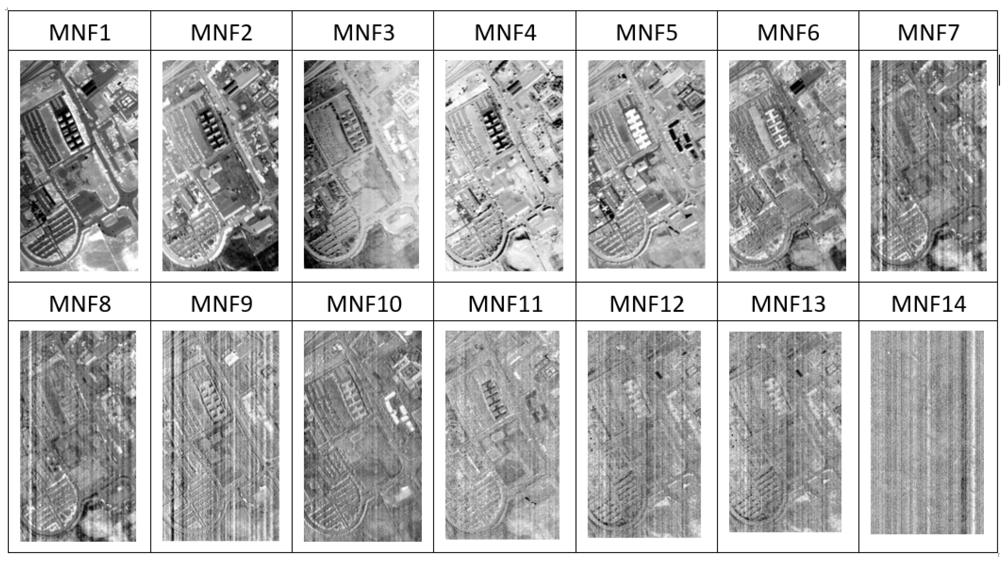
2.2. Frequency Transformation—Minimum Noise Fraction (MNF)

MNF was applied for dimensionality reduction in this study. MNF segregates noise from bands through modified principal-component analysis (PCA) by ranking images on the basis of signal-to-noise ratio (SNR) [39,49]. MNF defines the noise of each band as follows:
V { N i ( x ) } / V { S i ( x ) }
where N i ( x ) is the noise content of the xth pixel in the ith band, and S i ( x ) is the signal component of the corresponding pixel [43]. An image has p bands with gray levels S i ( x ) , i = 1 , 2 ,   p , where x is given as the image coordinate. A linear MNF transform is as follows:
Y i ( x ) = a i T S i ( x ) ,        i = 1 , , p
where   Y i ( x ) is the linear transform of the original pixel;   a i is the left-hand eigenfactor of Σ N i Σ 1 , and u i is the corresponding eigenvalue of a i , equal to the noise fraction in Y i ( x ) . u 1 u 2 u describes the ranking of MNFs by the image quality.

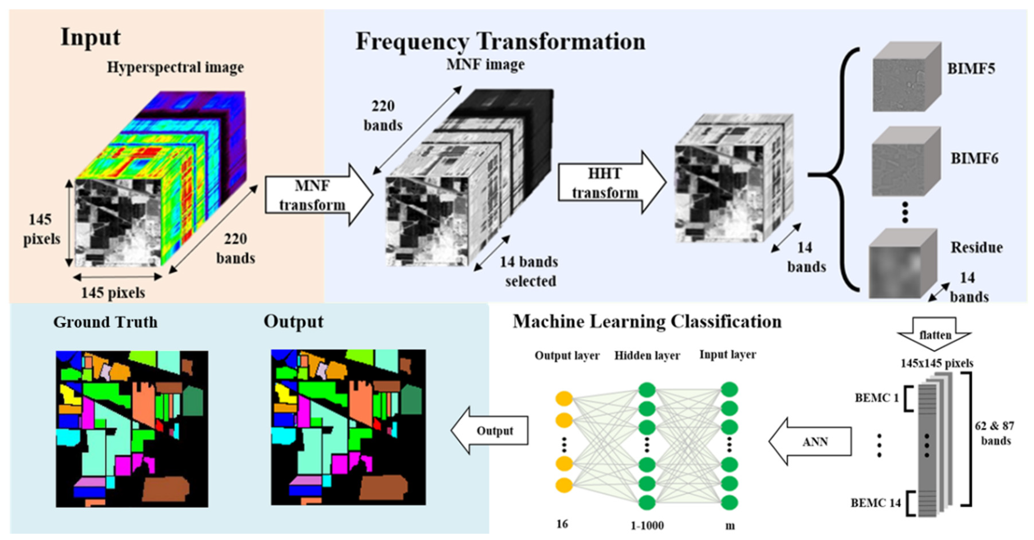
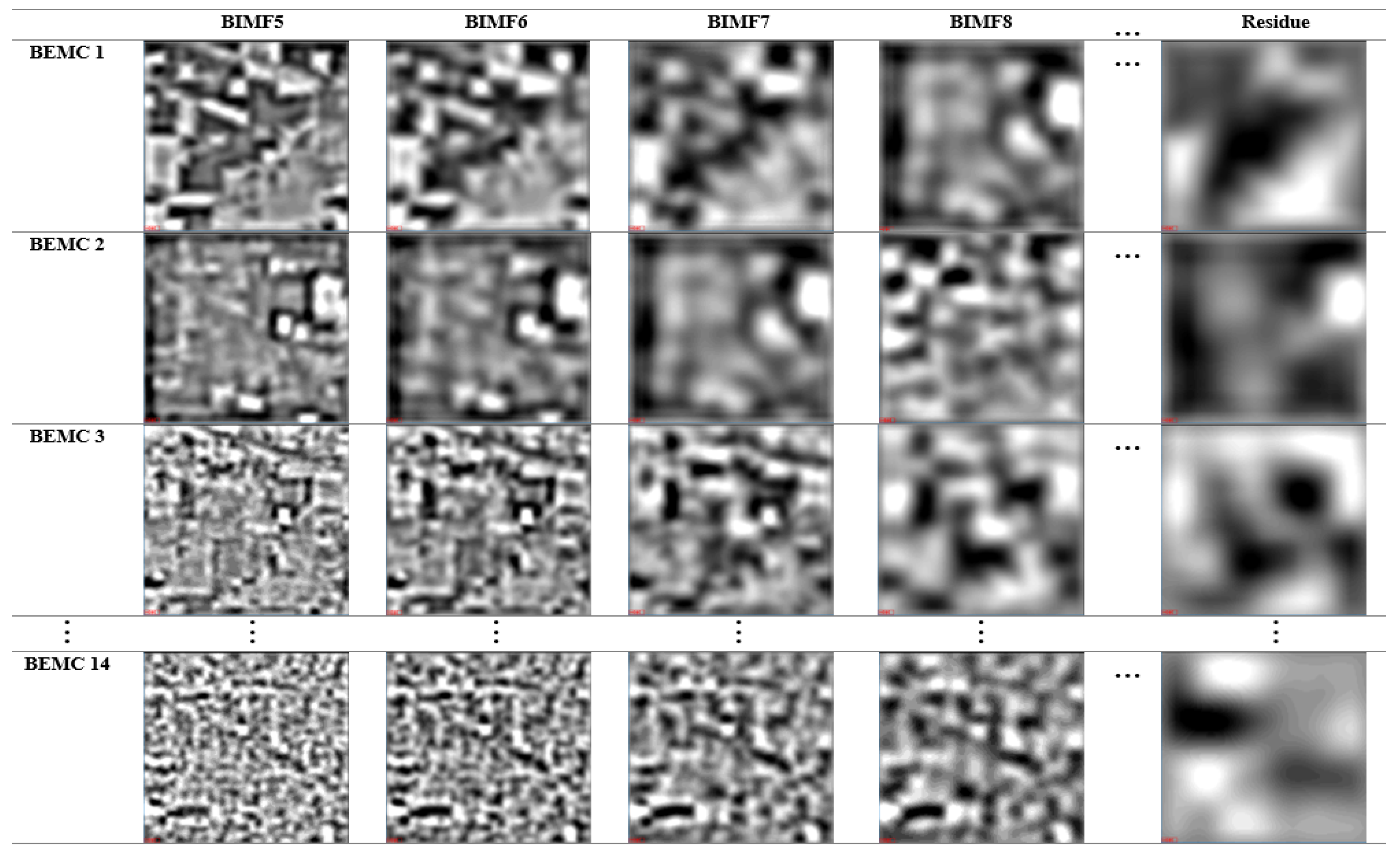
2.3. Frequency Transformation—Hilbert–Huang Transform (HHT)

FABEMD, a branch of HHT, was implemented to decompose the extracted features. FABEMD offers an efficient mathematical solution by using order-statistics filters to estimate the upper and lower envelopes and setting the screening iteration number for each two-dimensional intrinsic mode function (BIMF) to one. The primary process of FABEMD is described below [43,44,50].
A maximum-value map (LMMAX) and a minimum-value map (LMMIN) are generated by a two-dimensional array of local maxima and minima. Local extreme points are identified by the neighbor-kernel method and points with pixel values strictly above (below) all their neighbors are considered local maxima (minima). A commonly used 3 × 3 kernel was adopted because it produces more favorable local extremum detection results than a large kernel size [44]. When the extreme point is in the border and corner of the image, neighboring points within the kernel are ignored.
a m n { L o c a l   M a x i m u m      i f   a m n > a k l L o c a l   M i n i m u m      i f   a m n < a k l
where a m n is an element of the array located at the mth row and nth column, and Equations (4) and (5) represent k and l.
k = m w e x 1 2 : m + w e x 1 2 , ( k m )
l = n w e x 1 2 : n + w e x 1 2 , ( l m )  
where w e x × w e x is the neighboring kernel size for detecting extremum points. An illustration of the BEMCs with associated BIMFs and residue image of the IP dataset is shown in Figure 2.

2.4. Machine Learning Classification—Artificial Neural Networks (ANNs)

ANNs, a subset of machine learning, have already shown great promise in HSI classification. The network training was performed using the open-source software ffnet version 0.8.0 [51] with the standard sigmoid function and the truncated Newton method (TNC) used for gradient optimization in the hidden layer [52,53]. The number of neurons was set as equal to the number of input bands, and the maximum number of iterations was set to 5000. Fifty percent of the pixels from each class of the HSI were randomly selected to form the training dataset for the assessment of classification accuracy. The selection and assessment were implemented 20 times to obtain a relatively reasonable accuracy in the training dataset. Percentages of 10%, 20%, 40%, 60% of the pixels were randomly selected from the training dataset to represent the 5%, 10%, 20%, and 30% training samples.

3. Results & Discussion

3.1. Frequency Transformation—MNF+HHT Transform

Two frequency transformations were performed. First, a MNF transform was performed for noise and dimension reduction of the HSIs. The output images of the MNF transform were ranked by their signal-to-noise ratio (SNR) and image quality. In general, low-ordered MNF images contained higher SNR and image quality; therefore, the first 14 MNF images were extracted to give two image sets, MNF1–10 and MNF1–14, for comparison purposes. The rest of BIMFs and the residue image were composited for later ANN classification. Figure 2 shows the BIMFs and residue image for BEMCs 1–14. All BIMFs and residue images were derived directly from HHT transformation. Based on visual inspection, the image quality decreased with higher-ordered BIMFs as well as with higher-ordered BEMCs.

3.2. Machine Learning Classification—Training Sample Proportions

Four training sample proportions, 5%, 10%, 20%, and 30%, were tested with three categories of images (i.e., the original 220 bands of the IP dataset, two sets of MNF-transformed images, and two sets of MNF+HHT-transformed images) separately to investigate how changing training sample proportions would impact on the ANN’s classification performance. Two hundred neurons were used in the hidden layer of the ANN as a benchmark to test the classification performance.
Figure 3 shows the ANN classification results for the IP dataset, using 200 neurons of each proportion of training sample in each category of images. In general, the classification accuracy increased with the increase in training sample proportion, indicating the data-eager characteristics of ANNs. Additionally, despite the proportion of training samples, the MNF+HHT-transformed image sets displayed higher accuracy than the MNF-transformed images and the original 220 bands of the IP dataset, indicating that the data-frequency transformations by MNF and HHT significantly improved the classification accuracy.
Moreover, it was observed that MNF+HHT transformation remarkably reduced dependence on the amount of training data when using an ANN. For instance, in the situation of using a 5% training samples, the MNF1–10+HHT images and the MNF1–14+HHT images achieve 96.33% and 97.02% accuracies, respectively, which were 4.58% and 5.28% higher than the 91.75% accuracy achieved by the original 220 band Indian Pine images with a 30% training sample.
Furthermore, Figure 3 displays the results of 5% to 30% training sample proportions with the original 220 band IP dataset, MNF-transformed image sets, and MNF+HHT-transformed image sets. The pairwise T-test was performed to compare the 220 band set with MNF+HHT-transformed image sets. The statistical results showed that both MNF1–10+HHT and MNF1–14+HHT transformations produced significantly higher accuracy than classification in the original 220 band IP dataset (p-values 0.058 and 0.059, respectively; α = 0.10).
Larger improvements were observed for the MNF+HHT transformation shown in Figure 4. For example, MNF1–14+HHT transformation improved the accuracy from 62.17% to 97.02% for the ANN classification, which showed a 34.85% accuracy improvement, in contrast with the 27.79% improvement from 62.17% to 89.96% for the MNF1–14 image set.
To make a more rigorous comparison of the accuracy between MNF-transformed images and MNF+HHT-transformed images (Figure 4), with the 5% training sample, the accuracy of the MNF1–10+HHT-transformed images reached 96.33%, which was 5.93% higher than the 90.40% accuracy achieved by MNF transformation. With the 10%, 20%, and 30% training samples, the accuracies of the MNF1–10+HHT-transformed images were 6.01%, 5.62%, and 4.22% higher than that of the MNF1–10 images, respectively. Likewise, higher accuracies were found in the MNF+ HHT-transformation sets in the comparison of the MNF1–14+HHT and MNF1–14 images. With the 5% training sample, the accuracy of the MNF1–14+HHT-transformed images reaches 97.02%, which was 7.06% higher than the 89.96% accuracy achieved by MNF transformation. With the 10%, 20%, and 30% training samples, the accuracies of the MNF1–14+HHT-transformed images were 6.77%, 5.70%, 4.19%, and 3.41% higher than those of the MNF1–14 images, respectively.
For PaviaU dataset, a similar pattern to the IP dataset was observed, as shown in Figure 5 and Figure 6. As shown in Figure 5, the classification accuracy rose with the increase in training sample proportion. Likewise, the MNF+HHT-transformed image sets showed higher accuracy than the MNF-transformed images and the original 103 bands of the PaviaU dataset with any proportion of training samples, which highlights again that MNF and HHT transformations significantly improved the classification accuracy.
Moreover, it was also observed that MNF and HHT transformations successfully lowered the demand for training samples. When using 5% training samples, the MNF1–10+HHT images and the MNF1–14+HHT images achieved 93.58% and 92.44% accuracies, respectively, which was 1.45% and 0.31% higher than the 92.13% accuracy achieved by the original 103 band PaviaU image with a 30% training sample.
Additionally, Figure 6 displays the accuracy comparison of 5% to 30% training sample proportions with the original 103 bands of the PaviaU dataset, MNF-transformed image sets, and MNF+HHT-transformed image sets. Based on a pairwise T-test, the statistical results showed that MNF1–10, MNF1–10+HHT, and MNF1–14+HHT transformations produced significantly higher accuracies than classification in the original 103 band PaviaU dataset (p-value < 0.001).
Compared to the IP dataset, smaller but still positive improvements were observed for the MNF+HHT transformation, as shown in Figure 6. For example, MNF1–10+HHT showed improved accuracy from 87.64% to 93.58% for the ANN classification, which was a 5.94% accuracy improvement.

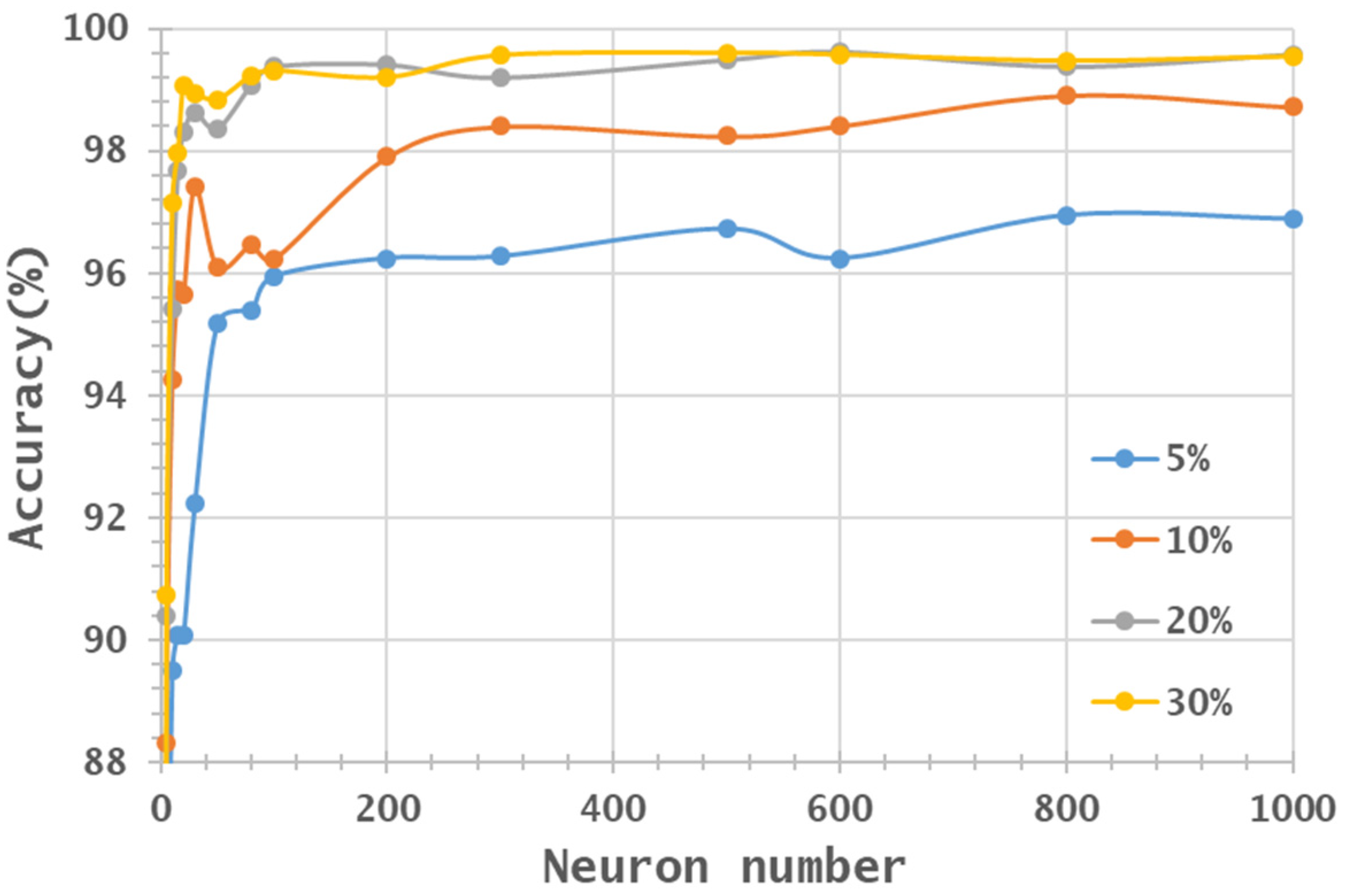
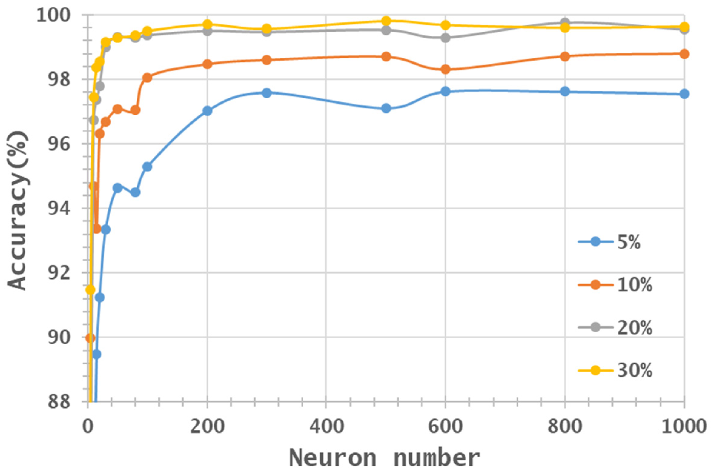
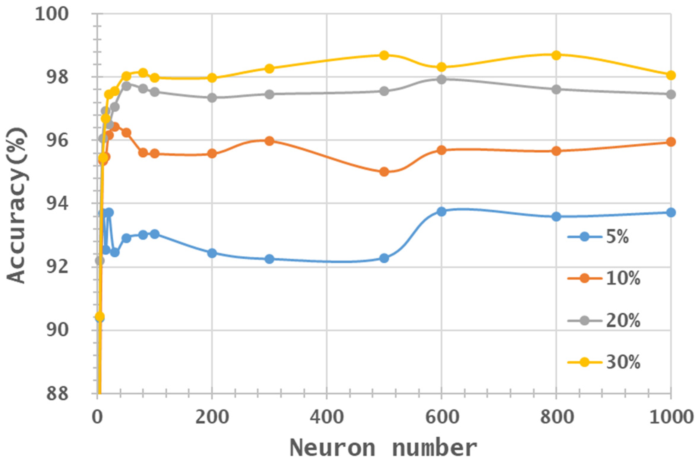
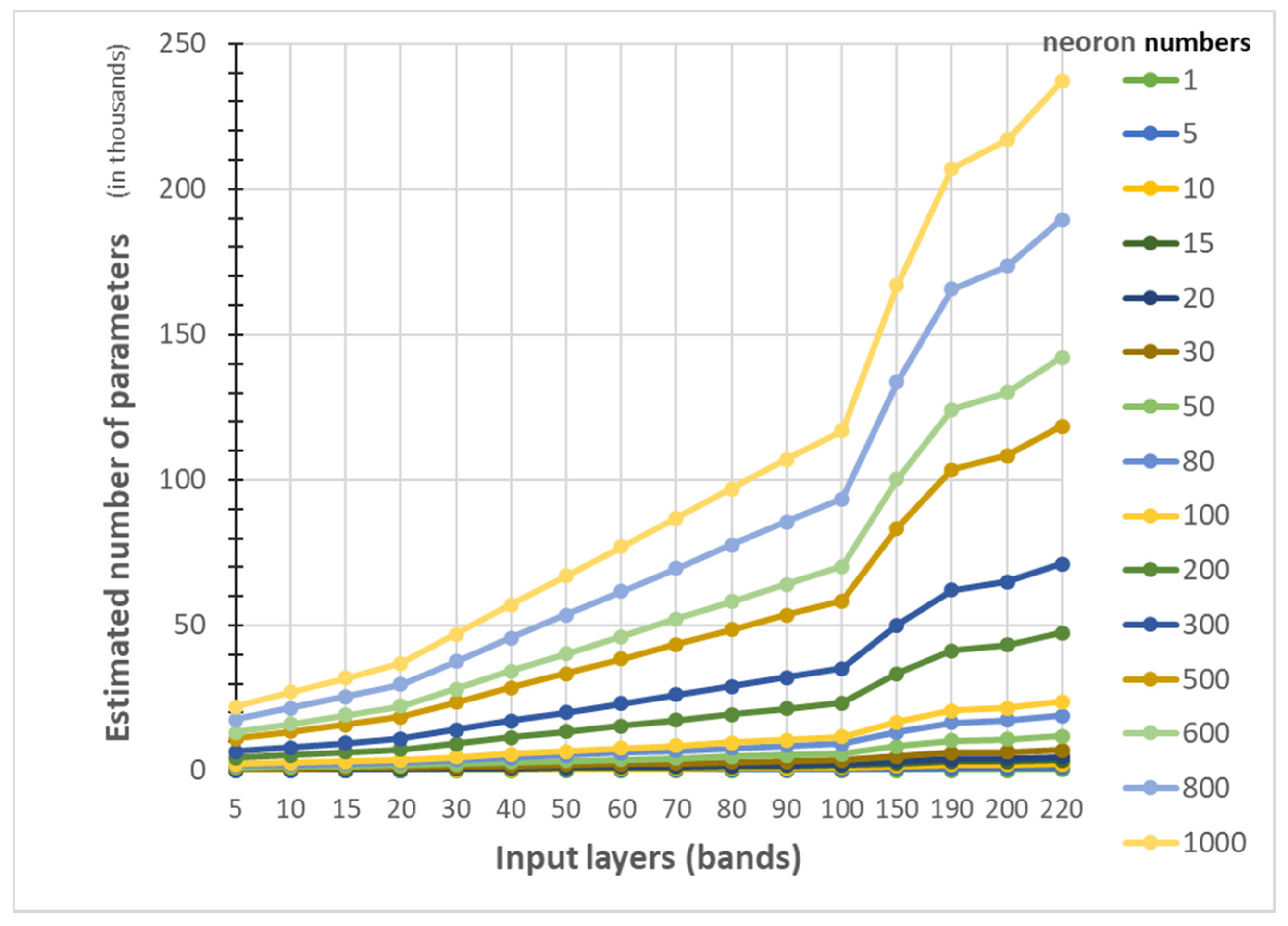
3.3. Machine Learning Classification—Neuron Numbers

For the purpose of understanding the influence of the number of neurons in the ANN on classification accuracy, two categories of images, MNF1–10+HHT and MNF1–14+HHT images, were compared in terms of classification performance, using 1 to 1000 neurons in the hidden layer with 5 %, 10%, 20%, and 30% training sample proportions. Table 1, Table 2, Table 3 and Table 4 show the results of the classification accuracy of MNF1–10+HHT and MNF1–14+HHT image sets for the IP and PaviaU datasets. The highest accuracy value in the corresponding training sample proportion column is shown in bold, and values above 95% are shaded in light gray. In comparison, values above 99% are shaded in dark gray.
For the IP dataset, as shown in Table 1, the MNF1–10+HHT image set with 5% and 10% training sample proportions, the highest accuracies of 96.94% and 98.91% occurred at 800 neurons. With 20% and 30% training sample proportions, the highest accuracies were found when the hidden layer had 600 and 500 neurons, respectively. In Table 2 of the Indian Pines MNF1–14+HHT image set, the highest accuracies in 5 %, 10%, 20%, and 30% training sample proportions appeared when the hidden layer had 600, 1000, 800, and 500 neurons, respectively. Based on the paired T-test, both MNF1–10+HHT and MNF1–14+HHT transformations produced significantly higher accuracies when more training samples were used.
For both the MNF1–10+HHT and MNF1–14+HHT image sets for the IP dataset, significantly higher accuracies were observed when using a 10% training sample than when using a 5% training sample (respectively, p-value = 0.0002, α = 0.01 and p-value = 0.0054, α = 0.01). Similarly, significantly higher accuracy was achieved when using a 20% training sample than when using a 10% training sample (p-value > 0.0001, α = 0. 01 and p-value = 0.0589, α = 0.10). However, no significant difference was found between 20% and 30% training sample proportions, which demonstrates the limitations in the accuracy improvement that can be achieved by increasing the training sample size. Besides, comparing the values of accuracy, the MNF1–14+HHT image set reached a value above 99% when the hidden layer used 30 neurons at a 20% training sample proportion, whereas the MNF1–10+HHT image set needed 80 neurons, which may support an inference that the MNF1–14+HHT images had more discriminative information in different classes to support better classification.
For the PaviaU MNF1–10+HHT image set, as shown in Table 3, above 95% accuracy was achieved using 5%, 10%, 20%, and 30% samples when the hidden layer had 30, 20, 15, and 10 neurons, respectively. With a 5% training sample proportion, the highest accuracy of 95.09% occurred at 30 neurons. With 10%, 20%, and 30% training sample proportions, the highest accuracies were found when the hidden layer had 800, 600, and 1000 neurons, respectively. As displayed in Table 4, the PaviaU MNF1–14+HHT image set achieved above 95% accuracy with 10 neurons using 10% to 30% training samples. The highest accuracies in the 5 %, 10%, 20%, and 30% training sample proportions appeared when the hidden layer has 600, 30, 600, and 800 neurons, respectively.
From a visual aspect, Figure 7, Figure 8, Figure 9 and Figure 10 represent the classification accuracy results of the IP and PaviaU MNF1–10+HHT and MNF1–14+HHT image sets with 5%, 10%, 20%, and 30% training sample proportions. Based on the structure of an ANN, the number of parameters for each layer was deliberated. First of all, the number of neurons in the hidden layer was set as equal to the number of input bands. Secondly, the number of parameters in the output layer was set to 16 due to the number of classes in the IP dataset. Therefore, the total parameters could be estimated according to the number of input bands. In the present study, 5 to 220 bands derived from the IP dataset were taken as the input layer, whereas the hidden layer had 1 to 1000 neurons. The output layer produced the probability of 16 classes. As shown in Figure 11, with an increasing number of input layers (bands), the associated estimated number of parameters rose exponentially when the neuron number increased. The rising of the estimated parameters was exaggerated if the number of neurons in the hidden layer increased. As the estimated parameters upsurge, the model becomes more complex and tends to over-fit when the number of available training samples is limited.
Figure 12 and Figure 13 show the maps generated from the best classification results of each training sample proportion. In general, the misclassified pixels can be observed around the boundaries of classification blocks. It is clear to see that the classification accuracy increased as the training sample proportion increases, as well as when the number of neurons increased. The 30% training sample proportion set produced the highest accuracy almost every tims. However, the increasing rate of accuracy was more apparent when the number of neurons was below 200. The accuracy improvement curve became relatively flat when more than 200 neurons were used. This result revealed that using more discriminative information from transformed images can reduce the number of neurons needed to adequately describe the data, as well as reducing the complexity of the ANN model.
Furthermore, several interesting results were observed based on the experiments with these two datasets. Compared to the IP dataset with 220 bands, the PaviaU dataset derived from ROSIS, processing 103 bands with nine classes, needed fewer neurons to achieve a similar classification accuracy. Regarding band selection, the performance of MNFs 1–14 was superior to that of MNFs 1–10 in the IP dataset, reflecting that MNFs 1–10 might have excluded some effective spectral information, whereas MNFs 1–10 showed superior performance to MNFs 1–14 in the PaviaU dataset (using 5% and 10% training samples), reflecting that MNFs 1–14 might have included ineffective spectral information and so decreased the classification accuracy. As shown in Figure 14, for the PaviaU dataset, the order of MNF images represents the spectral information of the scene. The MNF 1 to MNF 10 images illustrated better scene information than MNF 11 to MNF 14 based on a visual evaluation. In short, the PaviaU images needs less MNFs to achieve a similar classification accuracy than the IP image set did, due to its lower-dimensional spectral information.
For the IP dataset, the training data proportions of 5% and 10% resulted in unsatisfactory classification in a 220 band run due to some classes possessing only a few pixels, thus causing insufficient training. For example, the classes of “Oats”, “Hay-windrowed”, and “Alfalfa” possessed only 1, 2, and 3 pixels, respectively, in the 5% training data selection, which resulted in lower overall accuracy. However, the proposed method reached a high overall accuracy of 97.62% even with insufficient training data, such as the 5% selection, which proves its usability in situations with limited training data and high-dimensional spectral information.

4. Conclusions

To enhance HSI classification, this study proposes a process integrating MNF and HHT to reduce image dimensions and decompose images. Specifically, MNF and HHT function as feature extractor and image decomposer, respectively, to minimize the influences of noises and dimensionality. This study tested two variables, the number of neurons and training sample proportion, to evaluate the variation of ANN classification accuracy.
For both the IP and PaviaU hyperspectral datasets, the statistically significant classification accuracy improvement indicated that the proposed MNF+HHT process had excellent and stable performance. The major contributions and findings can be summarized as follows.
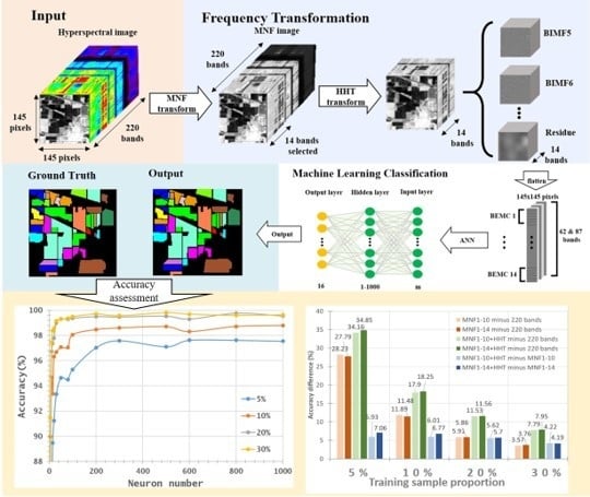
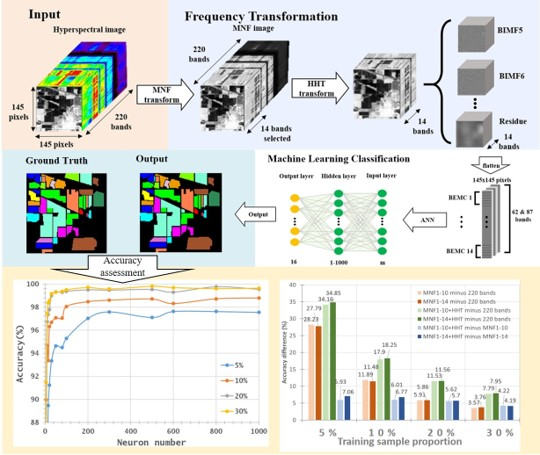
  • With the aim of solving two critical issues in HSI classification, the curse of dimensionality and the limited availability of training samples, this study proposes a novel approach by integrating MNF and HHT transformations into ANN classification. MNF was performed to reduce the dimensionality of HSI, and the decomposition function of HHT produced more discriminative information from images. After MNF and HHT transformations, training samples were selected for each land cover type with four proportions and tested using 1–1000 neurons in an ANN. For a comparison purpose, three categories of image sets, the original HSI dataset, MNF-transformed images (two sets), and MNF+HHT-transformed images (two sets) were compared regarding their ANN classification performances.
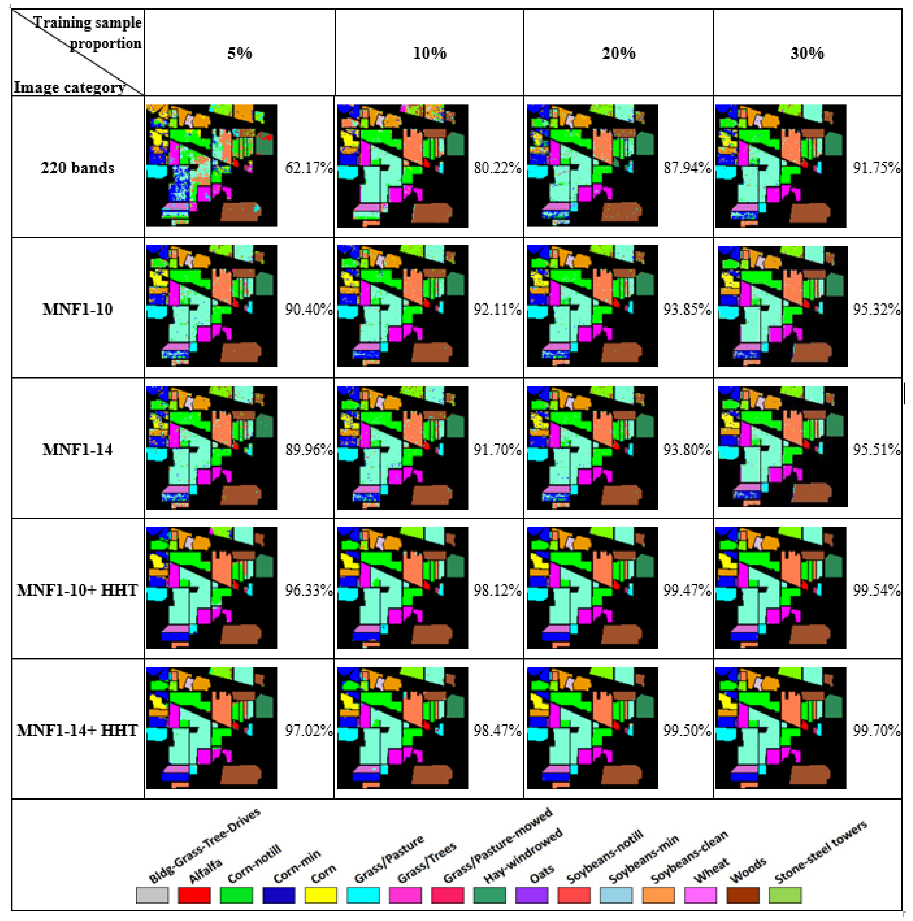
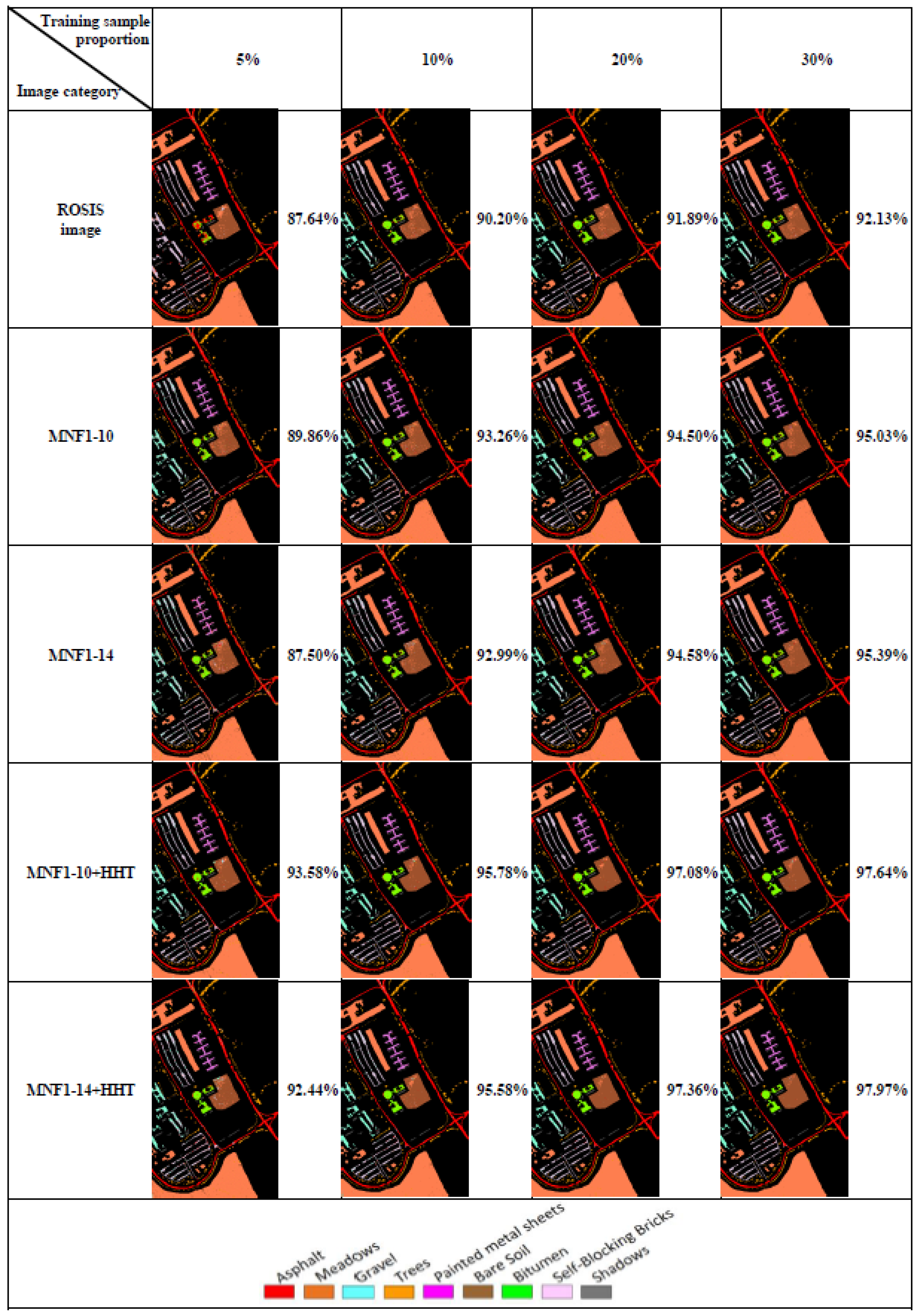
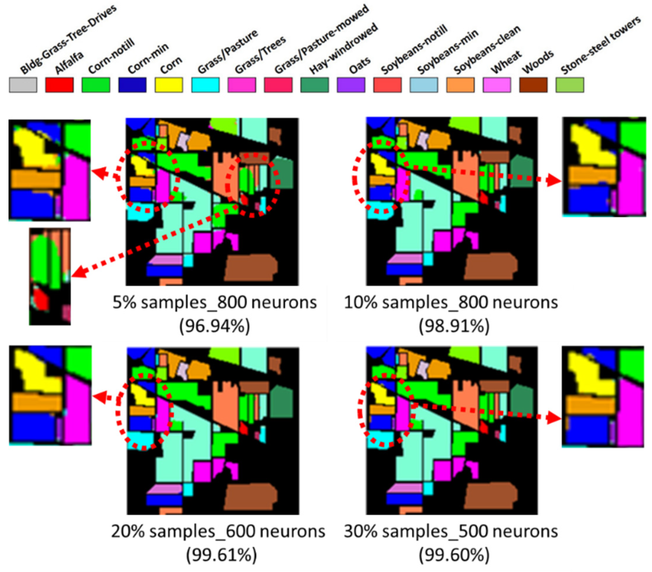
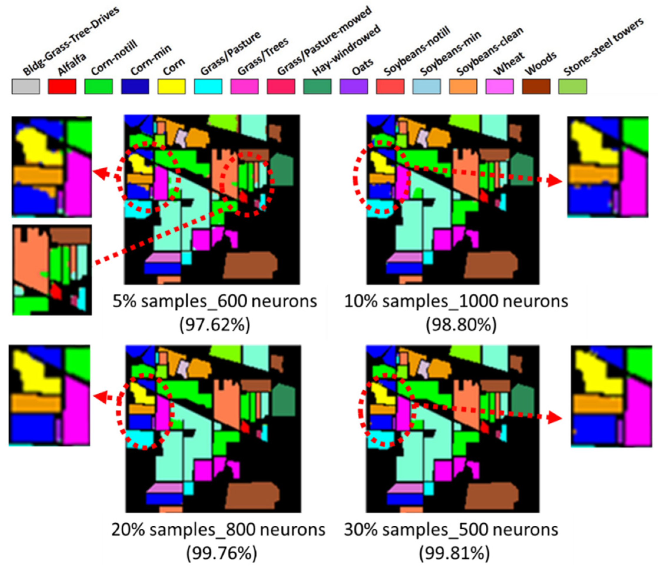
  • Two HSI datasets, the Indian Pines (IP) and Pavia University (PaviaU) datasets, were tested with the proposed method. The results showed that the IP MNF1–14+HHT-transformed images achieved the highest accuracy of 99.81% with a 30% training sample using 500 neurons, whereas the PaviaU dataset achieved the highest accuracy of 98.70% with a 30% training sample using 800 neurons. The results revealed that the proposed approach of integrating MNF and HHT transformations efficiently and significantly enhanced HSI classification performance by the ANN.
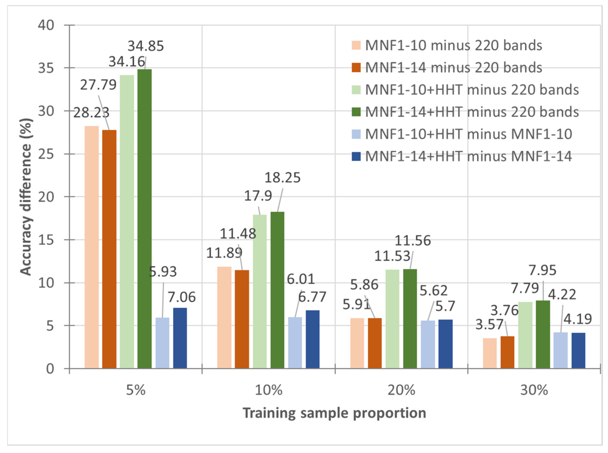
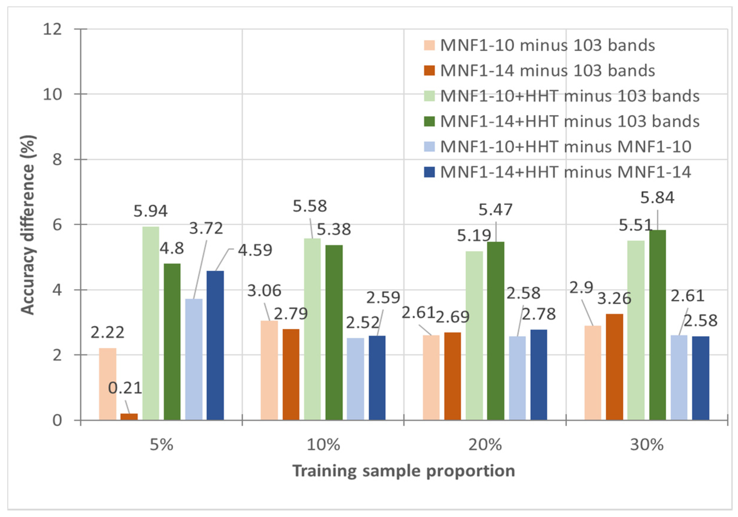
  • In general, the classification accuracy increased as the training sample proportion increased and as the number of neurons increased, indicating the data-eager characteristics of ANNs. The MNF+HHT transformed image sets also displayed the highest accuracy statistically. A large accuracy improvement, 34.85%, was observed for the IP MNF1–14+HHT image set compared with the original 220 band IP image using 5% training samples. However, no significant difference was found between 20% and 30% training sample proportions, which demonstrates the limitations in the accuracy improvement that can be achieved by increasing the sample size. The accuracy improvement of the PaviaU dataset was smaller but still positive. For the PaviaU dataset, 10 MNFs showed superior performance to 14 MNFs when using 5% and 10% training samples, which reflected that 14 MNFs might include ineffective spectral information and thus decrease the classification accuracy. The PaviaU image set needed fewer MNFs than the IP set did to achieve a similar classification accuracy, due to its lower-dimensional spectral information
  • Additionally, the accuracy improvement curve became relatively flat when more than 200 neurons were used for both datasets. This observation revealed that using more discriminative information from transformed images can reduce the number of neurons needed to adequately describe the data, as well as reducing the complexity of the ANN model.
  • The proposed approach suggests new avenues for further research on HSI classification using ANNs. Various DL-based methods such as semantic segmentation [54], manifolding learning, GANs, RNN, SAE, SLFN, ELM, or automatic feature-extraction techniques could be further investigated as future possible research directions.

Author Contributions

Conceptualization, M.-D.Y. and K.-H.H.; methodology, M.-D.Y. and K.-H.H.; software, M.-D.Y. and K.-H.H.; validation, M.-D.Y., K.-H.H., and H.-P.T.; formal analysis, M.-D.Y., K.-H.H., and H.-P.T.; writing—original draft preparation, K.-H.H., and H.-P.T.; writing—review and editing, M.-D.Y. and H.-P.T.; visualization, K.-H.H.; supervision, M.-D.Y. and H.-P.T.; project administration, M.-D.Y.; funding acquisition, M.-D.Y. All authors have read and agreed to the published version of the manuscript.

Funding

This research was partially funded by the Ministry of Science and Technology, Taiwan, under Grant Number 108-2634-F-005-003.

Acknowledgments

This research is supported through Pervasive AI Research (PAIR) Labs, Hsinchu 300, Taiwan, and “Innovation and Development Center of Sustainable Agriculture” from The Featured Areas Research Center Program within the framework of the Higher Education Sprout Project by the Ministry of Education (MOE) in Taiwan.

Conflicts of Interest

The authors declare no conflict of interest.

References

  1. Yang, M.-D.; Yang, Y.F.; Hsu, S.C. Application of remotely sensed data to the assessment of terrain factors affecting the Tsao-Ling landslide. Can. J. Remote Sens. 2004, 30, 593–603. [Google Scholar] [CrossRef]
  2. Yang, M.-D.; Su, T.C.; Hsu, C.H.; Chang, K.C.; Wu, A.M. Mapping of the 26 December 2004 tsunami disaster by using FORMOSAT-2 images. Int. J. Remote Sens. 2007, 28, 3071–3091. [Google Scholar] [CrossRef]
  3. Tsai, H.P.; Lin, Y.-H.; Yang, M.-D. Exploring Long Term Spatial Vegetation Trends in Taiwan from AVHRR NDVI3g Dataset Using RDA and HCA Analyses. Remote Sens. 2016, 8, 290. [Google Scholar] [CrossRef] [Green Version]
  4. Demir, B.; Erturk, S.; Güllü, M.K. Hyperspectral Image Classification Using Denoising of Intrinsic Mode Functions. IEEE Geosci. Remote Sens. Lett. 2010, 8, 220–224. [Google Scholar] [CrossRef]
  5. Taskin, G.; Kaya, H.; Bruzzone, L.; Kaya, G.T. Feature Selection Based on High Dimensional Model Representation for Hyperspectral Images. IEEE Trans. Image Process. 2017, 26, 2918–2928. [Google Scholar] [CrossRef]
  6. Romero, A.; Gatta, C.; Camps-Valls, G. Unsupervised Deep Feature Extraction for Remote Sensing Image Classification. IEEE Trans. Geosci. Remote Sens. 2015, 54, 1349–1362. [Google Scholar] [CrossRef] [Green Version]
  7. Ma, X.; Geng, J.; Wang, H. Hyperspectral image classification via contextual deep learning. EURASIP J. Image Video Process. 2015, 2015, 1778. [Google Scholar] [CrossRef] [Green Version]
  8. Kavzoglu, T. Increasing the accuracy of neural network classification using refined training data. Environ. Model. Softw. 2009, 24, 850–858. [Google Scholar] [CrossRef]
  9. Ratle, F.; Camps-Valls, G.; Weston, J. Semisupervised Neural Networks for Efficient Hyperspectral Image Classification. IEEE Trans. Geosci. Remote Sens. 2010, 48, 2271–2282. [Google Scholar] [CrossRef]
  10. Atkinson, P.M.; Tatnall, A.R.L. Introduction Neural networks in remote sensing. Int. J. Remote Sens. 1997, 18, 699–709. [Google Scholar] [CrossRef]
  11. Bruzzone, L.; Prieto, D. A technique for the selection of kernel-function parameters in RBF neural networks for classification of remote-sensing images. IEEE Trans. Geosci. Remote Sens. 1999, 37, 1179–1184. [Google Scholar] [CrossRef] [Green Version]
  12. Chen, Y.; Lin, Z.; Zhao, X.; Wang, G.; Gu, Y. Deep Learning-Based Classification of Hyperspectral Data. IEEE J. Sel. Top. Appl. Earth Obs. Remote Sens. 2014, 7, 2094–2107. [Google Scholar] [CrossRef]
  13. Guo, A.J.X.; Zhu, F. Spectral-Spatial Feature Extraction and Classification by ANN Supervised With Center Loss in Hyperspectral Imagery. IEEE Trans. Geosci. Remote Sens. 2018, 57, 1755–1767. [Google Scholar] [CrossRef]
  14. Ahmad, M. A Fast 3D CNN for Hyperspectral Image Classification. arXiv 2020, arXiv:2004.14152. [Google Scholar]
  15. Zhang, H.; Li, Y.; Zhang, Y.; Shen, Q. Spectral-spatial classification of hyperspectral imagery using a dual-channel convolutional neural network. Remote Sens. Lett. 2017, 8, 438–447. [Google Scholar] [CrossRef] [Green Version]
  16. Pantazi, X.E.; Moshou, D.; Bochtis, D. Intelligent Data Mining and Fusion Systems in Agriculture; Academic Press: Landon, UK, 2019. [Google Scholar]
  17. Ahmad, M.; Shabbir, S.; Oliva, D.; Mazzara, M.; Distefano, S. Spatial-prior generalized fuzziness extreme learning machine autoencoder-based active learning for hyperspectral image classification. Optik 2020, 206, 163712. [Google Scholar] [CrossRef]
  18. Hu, W.; Huang, Y.; Wei, L.; Zhang, F.; Li, H. Deep Convolutional Neural Networks for Hyperspectral Image Classification. J. Sens. 2015, 2015, 258619. [Google Scholar] [CrossRef] [Green Version]
  19. Ghamisi, P.; Chen, Y.; Zhu, X.X. A Self-Improving Convolution Neural Network for the Classification of Hyperspectral Data. IEEE Geosci. Remote Sens. Lett. 2016, 13, 1537–1541. [Google Scholar] [CrossRef] [Green Version]
  20. Guidici, D.; Clark, M.L. One-Dimensional Convolutional Neural Network Land-Cover Classification of Multi-Seasonal Hyperspectral Imagery in the San Francisco Bay Area, California. Remote Sens. 2017, 9, 629. [Google Scholar] [CrossRef] [Green Version]
  21. Wu, P.; Cui, Z.; Gan, Z.; Liu, F. Residual Group Channel and Space Attention Network for Hyperspectral Image Classification. Remote Sens. 2020, 12, 2035. [Google Scholar] [CrossRef]
  22. Lee, H.; Kwon, H. Contextual deep CNN based hyperspectral classification. In Proceedings of the 2016 IEEE International Geoscience and Remote Sensing Symposium (IGARSS), Beijing, China, 10–15 July 2016; pp. 3322–3325. [Google Scholar] [CrossRef]
  23. Li, Y.; Zhang, H.; Shen, Q. Spectral–Spatial Classification of Hyperspectral Imagery with 3D Convolutional Neural Network. Remot. Sens. 2017, 9, 67. [Google Scholar] [CrossRef] [Green Version]
  24. Haut, J.M.; Paoletti, M.E.; Plaza, J.; Li, J.; Plaza, J. Active Learning With Convolutional Neural Networks for Hyperspectral Image Classification Using a New Bayesian Approach. IEEE Trans. Geosci. Remote Sens. 2018, 56, 6440–6461. [Google Scholar] [CrossRef]
  25. Petersson, H.; Gustafsson, D.; Bergstrom, D. Hyperspectral image analysis using deep learning—A review. In Proceedings of the 2016 6th International Conference on Image Processing Theory, Tools and Applications (IPTA), Oulu, Finland, 12–15 December 2016. [Google Scholar] [CrossRef]
  26. Chen, Y.; Jiang, H.; Li, C.; Jia, X.; Ghamisi, P. Deep Feature Extraction and Classification of Hyperspectral Images Based on Convolutional Neural Networks. IEEE Trans. Geosci. Remote Sens. 2016, 54, 6232–6251. [Google Scholar] [CrossRef] [Green Version]
  27. Bhateja, V.; Tripathi, A.; Gupta, A. An Improved Local Statistics Filter for Denoising of SAR Images. In Recent Advances in Intelligent Informatics; Springer: Heidelberg, Germany, 2014; pp. 23–29. [Google Scholar] [CrossRef]
  28. Ahmad, M. Fuzziness-based Spatial-Spectral Class Discriminant Information Preserving Active Learning for Hyperspectral Image Classification. arXiv 2020, arXiv:2005.14236. [Google Scholar]
  29. Rasti, B.; Hong, D.; Hang, R.; Ghamisi, P.; Kang, X.; Chanussot, J.; Benediktsson, J.A. Feature Extraction for Hyperspectral Imagery: The Evolution from Shallow to Deep (Overview and Toolbox). IEEE Geosci. Remote Sens. Mag. 2020. [Google Scholar] [CrossRef]
  30. Hong, D.; Wu, X.; Ghamisi, P.; Chanussot, J.; Yokoya, N.; Zhu, X.X. Invariant Attribute Profiles: A Spatial-Frequency Joint Feature Extractor for Hyperspectral Image Classification. IEEE Trans. Geosci. Remote Sens. 2020, 58, 3791–3808. [Google Scholar] [CrossRef] [Green Version]
  31. Gao, L.; Zhao, B.; Jia, X.; Liao, W.; Zhang, B. Optimized Kernel Minimum Noise Fraction Transformation for Hyperspectral Image Classification. Remote Sens. 2017, 9, 548. [Google Scholar] [CrossRef] [Green Version]
  32. Brémaud, P. Fourier Transforms of Stable Signals. In Mathematical Principles of Signal Processing: Fourier and Wavelet Analysis; Springer Science & Business Media: New York, NY, USA, 2013; pp. 7–16. [Google Scholar] [CrossRef]
  33. Yang, M.-D.; Su, T.-C.; Pan, N.-F.; Liu, P. Feature extraction of sewer pipe defects using wavelet transform and co-occurrence matrix. Int. J. Wavelets Multiresolut. Inf. Process. 2011, 9, 211–225. [Google Scholar] [CrossRef]
  34. Xia, J.; Du, P.; He, X.; Chanussot, J. Hyperspectral Remote Sensing Image Classification Based on Rotation Forest. IEEE Geosci. Remote Sens. Lett. 2014, 11, 239–243. [Google Scholar] [CrossRef] [Green Version]
  35. Yang, M.-D.; Su, T.-C. Segmenting ideal morphologies of sewer pipe defects on CCTV images for automated diagnosis. Expert Syst. Appl. 2009, 36, 3562–3573. [Google Scholar] [CrossRef]
  36. Su, T.-C.; Yang, M.-D.; Wu, T.-C.; Lin, J.-Y. Morphological segmentation based on edge detection for sewer pipe defects on CCTV images. Expert Syst. Appl. 2011, 38, 13094–13114. [Google Scholar] [CrossRef]
  37. Fauvel, M.; Benediktsson, J.A.; Chanussot, J.; Sveinsson, J.R. Spectral and Spatial Classification of Hyperspectral Data Using SVMs and Morphological Profiles. IEEE Trans. Geosci. Remote Sens. 2008, 46, 3804–3814. [Google Scholar] [CrossRef] [Green Version]
  38. Luo, G.; Chen, G.; Tian, L.; Qin, K.; Qian, S.-E. Minimum Noise Fraction versus Principal Component Analysis as a Preprocessing Step for Hyperspectral Imagery Denoising. Can. J. Remote Sens. 2016, 42, 106–116. [Google Scholar] [CrossRef]
  39. Sun, Y.; Fu, Z.; Fan, L. A Novel Hyperspectral Image Classification Pattern Using Random Patches Convolution and Local Covariance. Remote Sens. 2019, 11, 1954. [Google Scholar] [CrossRef] [Green Version]
  40. Huang, N.E.; Shen, Z.; Long, S.R.; Wu, M.C.; Shih, H.H.; Zheng, Q.; Yen, N.-C.; Tung, C.C.; Liu, H.H. The empirical mode decomposition and the Hilbert spectrum for nonlinear and non-stationary time series analysis. Proc. R. Soc. A Math. Phys. Eng. Sci. 1998, 454, 903–995. [Google Scholar] [CrossRef]
  41. Chen, Y.; Zhang, G.; Gan, S.; Zhang, C. Enhancing seismic reflections using empirical mode decomposition in the flattened domain. J. Appl. Geophys. 2015, 119, 99–105. [Google Scholar] [CrossRef]
  42. Chen, Y.K.; Zhou, C.; Yuan, J.; Jin, Z.Y. Applications of empirical mode decomposition in random noise attenuation of seismic data. J. Seism. Explor. 2014, 23, 481–495. [Google Scholar]
  43. Chen, Y.; Ma, J. Random noise attenuation by f-x empirical-mode decomposition predictive filtering. Geophysics 2014, 79, V81–V91. [Google Scholar] [CrossRef]
  44. Linderhed, A. 2D empirical mode decompositions in the spirit of image compression. Wavelet Indep. Compon. Anal. Appl. IX 2002, 4738, 1–9. [Google Scholar] [CrossRef]
  45. Bhuiyan, S.M.A.; Adhami, R.R.; Khan, J. Fast and Adaptive Bidimensional Empirical Mode Decomposition Using Order-Statistics Filter Based Envelope Estimation. EURASIP J. Adv. Signal Process. 2008, 2008, 1–18. [Google Scholar] [CrossRef] [Green Version]
  46. Yang, M.-D.; Huang, K.-S.; Yang, Y.F.; Lu, L.-Y.; Feng, Z.-Y.; Tsai, H.P. Hyperspectral Image Classification Using Fast and Adaptive Bidimensional Empirical Mode Decomposition With Minimum Noise Fraction. IEEE Geosci. Remote Sens. Lett. 2016, 13, 1950–1954. [Google Scholar] [CrossRef]
  47. Yang, M.-D.; Su, T.-C.; Pan, N.-F.; Yang, Y.-F. Systematic image quality assessment for sewer inspection. Expert Syst. Appl. 2011, 38, 1766–1776. [Google Scholar] [CrossRef]
  48. Bernabé, S.; Marpu, P.; Plaza, J.; Mura, M.D.; Benediktsson, J.A. Spectral–Spatial Classification of Multispectral Images Using Kernel Feature Space Representation. IEEE Geosci. Remote Sens. Lett. 2014, 11, 288–292. [Google Scholar] [CrossRef]
  49. Nielsen, A.A. Kernel Maximum Autocorrelation Factor and Minimum Noise Fraction Transformations. IEEE Trans. Image Process. 2010, 20, 612–624. [Google Scholar] [CrossRef] [Green Version]
  50. Trusiak, M.; Wielgus, M.; Patorski, K. Advanced processing of optical fringe patterns by automated selective reconstruction and enhanced fast empirical mode decomposition. Opt. Lasers Eng. 2014, 52, 230–240. [Google Scholar] [CrossRef]
  51. Park, K.; Hong, Y.K.; Kim, G.H.; Lee, J. Classification of apple leaf conditions in hyper-spectral images for diagnosis of Marssonina blotch using mRMR and deep neural network. Comput. Electron. Agric. 2018, 148, 179–187. [Google Scholar] [CrossRef]
  52. Shang, Y.; Wah, B.W. Global optimization for neural network training. Computer 1996, 29, 45–54. [Google Scholar] [CrossRef] [Green Version]
  53. Hinton, G.E.; Salakhutdinov, R.R. Reducing the Dimensionality of Data with Neural Networks. Science 2006, 313, 504–507. [Google Scholar] [CrossRef] [Green Version]
  54. Yang, M.-D.; Tseng, H.-H.; Hsu, Y.-C.; Tsai, H.P. Semantic Segmentation Using Deep Learning with Vegetation Indices for Rice Lodging Identification in Multi-date UAV Visible Images. Remote Sens. 2020, 12, 633. [Google Scholar] [CrossRef] [Green Version]
Figure 1. The flow chart of the proposed classification process illustrated with the IP dataset.
Remotesensing 12 02327 g001
Figure 2. Illustration of the 14 sets of BEMCs with BIMFs and residue image for the IP dataset.
Remotesensing 12 02327 g002
Figure 3. Classification results with overall accuracy values for IP dataset original 220 band images, MNF-transformed images, and MNF+HHT-transformed images with four training sample proportions.
Remotesensing 12 02327 g003
Figure 4. Accuracy comparisons between the original 220 band IP dataset, the MNF-transformed image sets, and the MNF+HHT-transformed image sets.
Remotesensing 12 02327 g004
Figure 5. Classification results with overall accuracy values for PaviaU dataset original 103 band images, MNF-transformed images, and MNF+HHT-transformed images with four training sample proportions.
Remotesensing 12 02327 g005
Figure 6. Accuracy comparisons between the original 103 band PaviaU dataset, the MNF-transformed image sets, and the MNF+HHT-transformed image sets.
Remotesensing 12 02327 g006
Figure 7. Accuracy distribution of IP MNF1–10+HHT image set, varying with training sample proportion and hidden layers.
Remotesensing 12 02327 g007
Figure 8. Accuracy distribution of IP MNF1–14+HHT image set, varying with training sample proportion and hidden layers.
Remotesensing 12 02327 g008
Figure 9. Accuracy distribution of PaviaU MNF1–10+HHT image set, varying with training sample proportion and hidden layers.
Remotesensing 12 02327 g009
Figure 10. Accuracy distribution of PaviaU MNF1–14+HHT image set, varying with training sample proportion and hidden layers.
Remotesensing 12 02327 g010
Figure 11. Estimated number of parameters with the associated number of input layers (bands).
Remotesensing 12 02327 g011
Figure 12. IP MNF1–10+HHT image classification of the highest accuracies, varying with training sample proportions (the accuracy values are provided in parentheses).
Remotesensing 12 02327 g012
Figure 13. IP MNF1–14+HHT image classification of the highest accuracies, varying with training sample proportions (the accuracy values are provided in parentheses).
Remotesensing 12 02327 g013
Figure 14. MNF1 to MNF14 images of the PaviaU dataset.
Remotesensing 12 02327 g014
Table 1. Classification accuracy results of IP MNF1–10+HHT image set with different training sample proportions using 1 to 1000 neurons. The highest accuracy value in the corresponding training sample proportion column is shown in bold, and values above 95% are shaded in light gray. In comparison, values above 99% are shaded in dark gray.
ImageIndian Pine MNF1–10+HHT Training Sample Proportions
Neuron Numbers 5%10%20%30%
123.8523.8523.8547.45
581.5488.3190.4090.74
1089.4994.2795.4197.14
1590.0895.7397.6797.97
2090.0895.6598.3099.06
3092.2297.4198.6198.94
5095.1796.1098.3698.84
8095.4096.4699.0799.23
10095.9496.2499.3799.31
20096.2497.9099.4099.20
30096.2798.4099.1999.56
50096.7298.2499.4899.60
60096.2498.4199.6199.57
80096.9498.9199.3799.47
100096.8898.7299.5799.54
Paired T test5% vs. 10%: p-value 0.000235993 (α = 0.01)
10% vs. 20%: p-value 0.00000956567 (α = 0.01)
Table 2. Classification accuracy results of IP MNF1–14+HHT image set with different training sample proportions using 1 to 1000 neurons. The highest accuracy value in the corresponding training sample proportion column is shown in bold, and values above 95% are shaded in light gray. In comparison, the value above 99% is shaded in dark gray.
ImageIndian Pine MNF1–14+HHT Training Sample Proportions
Neuron Numbers 5%10%20%30%
123.8544.3147.3947.66
578.8289.9983.7591.49
1083.7394.7096.7497.45
1589.4893.3697.3898.36
2091.2596.3197.8098.54
3093.3596.6999.0199.15
5094.6397.0799.3199.29
8094.5197.0499.2899.36
10095.3098.0699.3799.50
20097.0298.4799.5099.70
30097.5998.6099.4799.57
50097.1198.7099.5399.81
60097.6298.3199.3099.69
80097.6298.7299.7699.60
100097.5598.8099.5599.64
Paired T test5% vs. 10%: p-value 0.00543679 (α = 0.01)
10% vs. 20%: p-value 0.0589095 (α = 0.10)
Table 3. Classification accuracy results of PaviaU MNF1–10+HHT image set with different training sample proportions using 1 to 1000 neurons. The highest accuracy value in the corresponding training sample proportion column is shown in bold, and values above 95% are shaded in light gray.
ImagePaviaU MNF1–10+HHT Training Sample Proportions
Neuron Number 5%10%20%30%
143.6065.5359.0043.60
586.2789.5387.3390.16
1093.5094.6094.9795.44
1593.9994.7996.2595.88
2093.6596.2896.2496.28
3095.0995.5396.5596.97
5093.2396.3697.4097.46
8093.8595.9197.1697.34
10093.8596.0997.0297.17
20093.5895.7897.0897.64
30093.4995.6497.0297.66
50093.4795.8797.2497.82
60093.7695.8997.6197.85
80093.6096.8696.9097.55
100092.9796.0997.0898.22
Paired T test5% vs. 10%: p-value 0.0193299 (α = 0.05)
Table 4. Classification accuracy results of PaviaU MNF1–10+HHT image set with different training sample proportions using 1 to 1000 neurons. The highest accuracy value in the corresponding training sample proportion column is shown in bold, and values above 95% are shaded in light gray.
ImagePaviaU MNF1–14+HHT Training Sample Proportions
Neuron Number 5%10%20%30%
166.1266.1965.8665.99
590.3987.6692.1990.43
1093.6895.3496.0595.45
1592.5395.4896.9396.69
2093.7396.1796.5097.46
3092.4696.4397.0797.56
5092.9196.2597.7398.04
8093.0095.6297.6498.14
10093.0395.5897.5497.98
20092.4495.5897.3697.97
30092.2495.9997.4698.27
50092.2895.0297.5698.68
60093.7595.6997.9398.31
80093.5895.6797.6298.70
100093.7195.9597.4798.07
Paired T test5% vs. 10%: p-value 0.000154062 (α = 0.001)
10% vs. 20%: p-value 0.0000633683 (α = 0.001)

