Noise-sensitivity Analysis and Improvement of Automatic Retrieval of Temperature and Emissivity Using Spectral Smoothness

Abstract

There are numerous algorithms that can be used to retrieve land surface temperature (LST) and land surface emissivity (LSE) from hyperspectral thermal infrared (HTIR) data. The algorithms are sensitive to a number of factors, where noise is difficult to handle due to its unpredictability. Although there is a lot of research regarding the influence of noise on retrieval errors, few studies have focused on the mechanism. In this study, we selected the automatic retrieval of temperature and emissivity using spectral smoothness (ARTEMISS) algorithm—the representative of the iterative spectral smoothness temperature-emissivity separation algorithm family—as the research object and proposed an improved algorithm. First, we analyzed the influence mechanism of noise on the retrieval errors of ARTEMISS in theory. Second, we carried out a simulation and inversion experiment and analyzed the relationship between instrument spectral resolution, noise level, the ARTEMISS parameter setting and the retrieval errors separately. Last, we proposed an improved method (resolution-degrade-based spectral smoothness algorithm, RDSS) based on the mechanism and law of the influence of noise on retrieval errors and provided corresponding suggestions on instrument design. The results show that RDSS improves the accuracy of temperature inversion and is more effective for thermal infrared data with a high noise level and high spectral resolution, which can reduce the LST inversion error by up to 0.75 K and the LSE median absolute deviation (MAD) by 31%. In the presence of noise in HTIR data, the RDSS algorithm performs better than the ARTEMISS algorithm in terms of temperature-emissivity separation.

1. Introduction

Land surface temperature (LST) and land surface emissivity (LSE) are two key physical parameters characterizing the state of the land surface, which are applied in various areas such as mineral mapping [1,2,3], gas plume detection [4], soil moisture inversion [5] and oil-film thicknesses measurement [6]. The LST is sensitive to the external environment and reflects the energy budget of an object during a period; the LSE, determined by the object itself, reflects its physical and chemical properties. The LST and LSE of an object can be simultaneously derived from thermal infrared (generally 8–14 μm) data through a temperature-emissivity separation (TES) algorithm. TES is a crucial issue in thermal infrared remote sensing, which can be seen as an underdetermined equation problem, i.e., obtaining N+1 unknowns (N emissivities at each band and one temperature) by solving N equations (one sensor output radiance with N bands). Consequently, it needs at least one additional constraint to make the underdetermined equations solvable.

For thermal infrared data with low or medium spectral resolution, LST is the principal retrieval goal compared with LSE. In this case, the primary task of TES algorithms for multiband thermal infrared data is to determine LSE. Many algorithms were developed for the inversion of LST from multispectral thermal infrared data, such as the split-window method [7], grey body emissivity [8], reference channel method [9], normalized emissivity method (NEM) [10,11], temperature independent spectral indices (TISI) [12], spectral ratio method [13], NDVI-based emissivity method (NBEM) [14,15,16,17] and advanced spaceborne thermal emission and reflection radiometer temperature-emissivity separation (ASTER TES) [18]. Among them, NBEM, TISI and ASTER TES are widely used methods [19]. Based on the relationship between NDVI and LSE, NBEM determines the LSE at specific bands with the help of visible near-infrared data. The ASTER TES method iteratively adjusts the average emissivity according to the empirical relationship between the change range of emissivity and the average emissivity to obtain the optimal LST. TISI transforms ground-leaving radiance under some approximation of the Planck function to make it reflect the spectral shape of emissivity. The day and night algorithm, based on TISI, has obtained good results on LST inversion of multi-band thermal infrared remote-sensing data [17]. TISI is theoretically suitable for thermal infrared remote sensing data of any spectral resolution; however, it cannot obtain absolute values of the retrieval emissivity spectrum. Therefore, TISI requires other data or theoretical constraints to solve the problem. The improvement of hyperspectral thermal infrared (HTIR) remote sensing technology brings new opportunities for the development of thermal infrared remote sensing. Unlike multi-spectral remote sensing, HTIR remote sensing is applied to retrieve not only LST but also LSE more accurately, which gives full play to the role of LSE on the fields of classification, identification and parameter inversion of the land surface (especially urban land surfaces of various types). As a result, the application scenarios of HTIR remote sensing are different to those of multispectral thermal infrared remote sensing. To adapt to new application scenarios, the goal of TES of HTIR remote sensing is to obtain the LST and LSE with the highest accuracy under the smallest number of universal and reasonable additional constraints. At present, scholars have proposed or improved a number of TES algorithms for HTIR data [20,21,22,23,24,25,26,27,28,29,30,31,32,33,34,35]. Unlike multispectral thermal infrared inversion methods, most TES algorithms for HTIR data have far fewer constraints. One well-known assumption of HTIR TES algorithms is that the LSE of most objects [36] is much smoother than the spectral curve of atmospheric downwelling radiance.

Iterative spectrally smooth temperature-emissivity separation (ISSTES) [21] is a representative TES algorithm based on the concept of spectral smoothness for HTIR data. ISSTES uses a smoothness index as a cost function measuring the atmospheric residue in the estimated LSE, and iteratively optimizes the estimated LST until the cost function is minimized and the corresponding LSE is considered optimally smoothed. The automatic retrieval of temperature and emissivity using spectral smoothness (ARTEMISS) improved ISSTES [22] by updating its cost function. ARTEMISS uses the standard deviation of the estimated at-sensor radiance and true at-sensor radiance as the cost function, instead of the absolute deviation of the estimated LSE and true LSE. Based on ARTEMISS, the quick temperature-emissivity separation (QTES) algorithm [23] was modified to retrieve LST and LSE from HTIR data measured near the ground. QTES uses a narrow spectral range (9.5–10 μm) instead of the entire spectral range of data when searching for the optimal temperature. In addition to the three algorithms proposed by Borel mentioned above, researchers have successively proposed many other TES algorithms based on the concept of spectral smoothness. The spectral smoothness method (SpSm) [24] uses the first derivative of estimated LSE spectrum as cost function. The downwelling radiance residual index (DRRI) [25] algorithm uses downwelling radiance residual index to measure roughness of LSE curve on several selected three-channel groups. The correlation-based temperature and emissivity separation (CBTES) method [26] constructs a cost function to measure the correlation between the estimated LSE and the atmospheric downwelling radiation, based on the concept that LSE is not directly related to atmospheric downwelling radiation, but when estimated LST is not accurate, estimated LSE will include residual atmospheric absorption information. The stepwise refining temperature and emissivity separation (SRTES) [27] considers self-emitting radiation of the land surface a function of wavenumber in a narrow spectral range, where LSE can be seen as a constant and the Planck function can be expressed in a linear form. However, atmospheric downwelling radiation still contains unignorable atmospheric absorption features. SRTES utilizes the residual atmospheric downwelling radiation of calculated self-emitting radiation as a criterion and obtains both the LSE at specified bands and the LST by the stepwise refining method. The correlation-wavelet method [28] considers the land surface self-emission curve as a fundamental-frequency signal and atmospheric downwelling radiance as a high-frequency signal, and obtains the land surface self-emission from ground-leaving radiance by filtering out the atmospheric characteristics based on the spectral smoothness concept. The correlation-wavelet method calculates the correlation between the emissivity curves calculated by taking into the atmospheric downwelling radiance and by direct wavelet filtering without considering atmospheric downwelling radiance. At the maximum correlation, the corresponding temperature is seen as the optimal retrieval temperature. Meanwhile, the emissivity curve is synthesized by wavelet signals of different scales whose proportion is calculated based on the correlation. A TES algorithm for low-emissivity materials [29] is based on the bias characteristic of atmospheric downwelling radiance, namely when retrieval LSE deviates from its true value, atmospheric downwelling radiance also deviates from its true value and the deviations are the same at the bands of the atmospheric absorption peak and valley. Some researchers have tried to reduce the unknowns of equations by reducing the dimensions of the emissivity, making the underdetermined equations solvable. One way to reduce the dimensionality is to divide the emissivity curve into several segments, each of which is the linear function of the wavelength. Based on the segmented linear constraints, three TES methods have been proposed, namely, the linear spectral emissivity constraint (LSEC) [30], the improved LSEC (I-LSEC) [31] and the pre-estimate shape LSEC (PES-LSEC) [32], which all take the sum of squared residuals of the estimated and true ground-leaving radiance as cost function. Another way to reduce the dimensionality is using the wavelet transform. The wavelet transform method for separating temperature and emissivity (WTTES) [33], which expresses LSE as a function of low-frequency wavelet coefficients, reduces the number of unknowns from N + 1 to N/2 + 1, and iteratively searches for the optimal wavelet coefficient and LST. The multi-scale wavelet-based TES algorithm (MSWTES) [34] is based on the fact that both high frequencies of ground-leaving radiance and the LSE calculated according to inaccurate LST are closely correlated with the atmospheric downwelling radiance. From the perspective of the spectral curve, the above TES algorithms follow similar basic concepts. For eliminating the influence of the “thorns” of a curve due to atmospheric absorption lines, the TES algorithms first aim to obtain a degraded approximate spectral curve close to the true spectral curve. For example, ISSTES estimates the LSE from equations directly; LSEC and WTTES estimate LSE after modifying its expression. Then, they search for the optimal LST, which minimizes the cost function and calculates its corresponding LSE as the final retrieval LSE. In addition to the idea of spectral smoothness, there is a new idea from the perspective of statistics, which assumes that the LSE spectra of natural and man-made materials can be well represented in a given subspace of the original data space. Based on the new idea, the dictionary subspace based temperature and emissivity separation (D-SBTES) [35,36] uses a singular value decomposition to extract the basis matrix of the subspace from the emissivity spectra dictionary to obtain the retrieval emissivity. However, D-SBTES suffers from several factors, such as noise, the rank of basis matrix adopted to address the emissivity subspace and the true land surface temperature, and it is more suitable for high-emissivity objects.

Overall, spectral smoothness has been a reasonable strategy widely used in the field of TES. Among the TES algorithms mentioned above, the most commonly used cost function is the standard deviation of the simulated at-sensor radiance and true at-sensor radiance, and a classic and common method to approximately process the LSE curve is the boxcar average. Therefore, for this study we researched ARTEMISS, which is the representative algorithm of the spectral smoothness TES family and has first-rate performance.

There are many impact factors to the performance of a TES algorithm for HTIR data, mainly including (1) sensor-related parameters (e.g., sensor altitude, spatial resolution, spectral range, spectral resolution and instrument noise), (2) data pre-processing (before TES) related residual errors (e.g., radiation calibration, spectral calibration and atmospheric correction) and (3) the algorithm’s limitations (e.g., the adopted assumptions or constraints) [37,38,39,40,41,42,43,44,45,46,47,48]. The sensor altitude affects the amount of atmospheric radiation entering the sensor. The higher the sensor altitude, the greater the inversion error [37,44]. If the spatial resolution is low, non-isothermal mixed pixels will appear in the thermal infrared hyperspectral image, which makes it difficult to separate the temperature emissivity accurately [39,41,42]. The spectral range of 7.5–8 μm, containing dense atmospheric absorption lines, is usually used to retrieve atmospheric parameters; however, the inversion requires a sufficient spectral resolution. The spectral range of 8–12.5 μm is usually used to retrieve the LST and LSE; the higher the spectral resolution, the smaller the retrieval errors [42,43]. A sufficient signal-to-noise ratio is necessary to obtain a unique solution for TES, and the retrieval error increases linearly with instrument noise [37,40,42]. The radiation calibration needs to have sufficient accuracy in order to make the simulated and measured radiance match [42]. The spectral calibration error greatly affects the temperature and emissivity errors even if the atmospheric correction has no error [40,45,46,47,48]. The influence of atmospheric correction errors (atmospheric upwelling radiance, atmospheric downwelling radiance and atmospheric transmittance) on the retrieval results varies by the TES algorithm. Among the three atmospheric parameters, atmospheric downwelling radiance has most of the influence on retrieval errors, especially for low-emissivity objects [41,43,45,46]. The adopted cost function is a mathematical expression of the adopted assumption for a TES algorithm, which certainly affects algorithm performance, regardless of whether the algorithm solves the underdetermined problem by increasing the constraints (e.g., spectral smoothness assumption) or reducing unknowns (e.g., piecewise linear constraint) [37,38,44,47,48].

The above factors, excluding the algorithm’s limitations, can be classified as systematic errors and random errors. The systematic errors can be reduced or removed by some correction methods based on the study of error patterns. For example, besides laboratory calibration, scene-based spectral calibration is able to improve further the spectral calibration accuracy of the field-measured data, which selects some atmospheric absorption channels as the reference channel to perform spectral calibration on the measured data, and the minimum error of the center wavelength shift is within 1 nm [49]. The sensor altitude, spectral range and resolution depend on the equipment development level and the external conditions during data acquisition. They mainly affect errors of the atmospheric parameters (input parameters for separating temperature and emissivity), and the accuracy of atmospheric correction increases with the improvement of technology [40,50,51]. The random errors, however, are much more difficult to deal with. Like noise, it is uncontrollable and limited by the detector technology, and it is difficult to remove the noise non-destructively after data acquisition. Therefore, the influence of random errors on the TES algorithms is also widely researched [25,26,27,28,30,31,32,37,40,41,42,43,44,47,48]. However, most research on this issue has been about how much noise causes the temperature and emissivity inversion errors, and only a few studies have focused on the influence mechanism of noise on the TES algorithms.

Here, we selected the ARTEMISS algorithm—a representative of the iterative spectral smoothness TES algorithm family with a good application effect—as the research object. The influence mechanism of noise on the retrieval errors of ARTEMISS is derived from the cost function. The relationships between the instrument spectral resolution, noise level, the ARTEMISS parameter setting and the retrieval errors are investigated through simulation experiment. On the basis of the mechanism and law of the influence of noise on the retrieval errors obtained from the experiment, the resolution-degrade-based spectral smoothness (RDSS) algorithm, an improved method, is proposed. Corresponding suggestions on the instrument design are also provided. Section 1 reviews TES algorithms and impact factors. Section 2 theoretically analyzes how noise affects the retrieval results of ARTEMISS. Section 3 describes the data simulation experiment, implementation of TES and the evaluation metrics for the retrieval results (Section 3.1) and the results of a sensitivity analysis of ARTEMISS regarding noise and smoothing window size (Section 3.2). Section 4 proposes the RDSS algorithm based on ARTEMISS, and presents the validation results. Section 5 and Section 6 present the discussion and conclusions, respectively.

2. Background

The temperature-emissivity separation is based on radiative transfer theory. Ignoring multiple scattering, the radiative transfer equation (RTE) [9,52,53] is as follows:

$$L\left({\lambda }_i,T\right)=L_g\left({\lambda }_i,T\right)\tau \left({\lambda }_i\right)+L_u\left({\lambda }_i\right)$$

(1)

$$L_g\left({\lambda }_i,T\right)=\epsilon \left({\lambda }_i\right)B\left({\lambda }_i,T\right)+\left[1-\epsilon \left({\lambda }_i\right)\right]L_d\left({\lambda }_i\right)$$

(2)

$$B\left({\lambda }_i,T\right)=\frac{c_1}{{\lambda }_i{}^5\cdot exp\left(\frac{c_2}{{\lambda }_{i}T}-1\right)}$$

(3)

where $L\left({\lambda }_i,T\right)$ is the at-sensor radiance at i-th band and LST of T, $i\in \left[1,N\right]$; N is the number of bands; $L_g\left({\lambda }_i,T\right)$ is the ground-leaving radiance, including the object’s self-emitting radiance and reflected atmospheric downwelling radiance; $L_u\left({\lambda }_i\right)$ is the atmospheric upwelling radiance; $\tau \left({\lambda }_i\right)$ is the atmospheric transmittance; $\epsilon \left({\lambda }_i\right)$ is the land surface emissivity; $B\left({\lambda }_i,T\right)$ is the blackbody radiance at T and $L_d\left({\lambda }_i\right)$ is the atmospheric downwelling radiance.

The original ARTEMISS algorithm includes two parts: atmospheric correction and temperature-emissivity separation. This study focuses on the influence of instrument noise on the retrieval LST and LSE of ARTEMISS. Therefore, this study only discusses the temperature-emissivity separation process of ARTEMISS, assuming the three atmospheric parameters ($\tau \left({\lambda }_i\right)$, $L_d\left({\lambda }_i\right)$ and $L_u\left({\lambda }_i\right)$) known and without errors. Then, we know $L_g\left({\lambda }_i,T\right)$ according to Equation (1). Given temperature estimation $\widehat{T}$, we can obtain the LSE according to Equation (2). The emissivity is calculated by,

$$\widehat{\epsilon }\left({\lambda }_i\right)=\frac{L_g\left({\lambda }_i,T\right)-L_d\left({\lambda }_i\right)}{B\left({\lambda }_i,\widehat{T}\right)-L_d\left({\lambda }_i\right)}$$

(4)

where $\widehat{\epsilon }\left({\lambda }_i\right)$ is the LSE estimation and $B\left({\lambda }_i,\widehat{T}\right)$ is the blackbody radiance at $\widehat{T}$.

According to the concept of spectral smoothness, the goal of ARTEMISS is to find an optimal LST estimation where the corresponding LSE is the smoothest. ARTEMISS uses the standard deviation of estimated at-sensor radiance and true at-sensor radiance as the cost function. When the cost function reaches the minimum, the corresponding LST estimation is the optimal LST. The process of ARTEMISS temperature-emissivity separation is as follows:

Given an LST estimation, the LSE estimation can be calculated using Equation (4); then, a boxcar average is performed on it and one can obtain the smoothed LSE estimation $\overline{\widehat{\epsilon }}\left({\lambda }_i\right)$:

$$\overline{\widehat{\epsilon }}\left({\lambda }_i\right)=\frac{1}{3}{\displaystyle \sum }_{j=i-1}^{i+1}\widehat{\epsilon }\left({\lambda }_j\right)$$

(5)

Then, the estimated at-sensor radiance, $L_{fit}(\lambda ,\widehat{T},\overline{\widehat{\epsilon }})$ is calculated according to the RTE:

$$L_{fit}(\lambda ,\widehat{T},\overline{\widehat{\epsilon }})=\widehat{\epsilon }\left(\lambda \right)B\left(\lambda ,T\right)\tau \left(\lambda \right)+\left[1-\widehat{\epsilon }\left(\lambda \right)\right]L_d\left(\lambda \right)\tau \left(\lambda \right)+L_u\left(\lambda \right)$$

(6)

Then, the standard deviation (cost function) of the estimated at-sensor radiance and the true at-sensor radiance is calculated:

$$\sigma (\widehat{T},\overline{\widehat{\epsilon }})=\sigma (L_{fit}(\lambda ,\widehat{T},\overline{\widehat{\epsilon }})-L(\lambda ,\widehat{T},\overline{\widehat{\epsilon }}))$$

(7)

We iteratively cycle through Equations (5)–(7) until the cost function reaches the minimum, and the corresponding temperature is seen as the optimal LST. Then we obtain the retrieval emissivity with the optimal temperature through Equation (4).

The above processes do not consider instrument noise. In fact, the output radiance of the thermal infrared hyperspectral sensor inevitably includes instrument noise. Instrument noise is a kind of random noise. In this study, the instrument noise is represented by additive Gaussian white noise, and the bands are uncorrelated. That is, to the right side of in Equation (1), add a noise term $\eta \left({\lambda }_i\right)$. Accordingly, to the right side of in Equation (2), also add a noise term $\frac{\eta \left({\lambda }_i\right)}{\tau \left({\lambda }_i\right)}$. Then $\widehat{\epsilon }\left({\lambda }_i\right)$ in Equation (4) becomes,

$$\begin{array}{cc}\hfill \widehat{\epsilon }\left({\lambda }_i\right)& =\frac{\left[B\left({\lambda }_i,T\right)-L_d\left({\lambda }_i\right)\right]\epsilon \left({\lambda }_i\right)+\frac{\eta \left({\lambda }_i\right)}{\tau \left({\lambda }_i\right)}}{B\left({\lambda }_i,\widehat{T}\right)-L_d\left({\lambda }_i\right)}\hfill \\ & =\frac{B\left({\lambda }_i,T\right)-L_d\left({\lambda }_i\right)}{B\left({\lambda }_i,\widehat{T}\right)-L_d\left({\lambda }_i\right)}\epsilon \left({\lambda }_i\right)+\frac{\frac{\eta \left({\lambda }_i\right)}{\tau \left({\lambda }_i\right)}}{B\left({\lambda }_i,\widehat{T}\right)-L_d\left({\lambda }_i\right)}\hfill \end{array}$$

(8)

where $\widehat{\epsilon }\left({\lambda }_i\right)$ and $\epsilon \left({\lambda }_i\right)$ are the estimated emissivity and its true value respectively and $\widehat{T}$ and $T$ are the estimated temperature and its true value respectively.

For simplicity, $\widehat{\epsilon }\left({\lambda }_i\right)$, $\epsilon \left({\lambda }_i\right)$, $B({\lambda }_i,\widehat{T})$, $B\left({\lambda }_i,T\right)$, $\tau \left({\lambda }_i\right)$, $L_u\left({\lambda }_i\right)$, $L_d\left({\lambda }_i\right)$ and $\eta \left({\lambda }_i\right)$ will be abbreviated in the following equations as ${\widehat{\epsilon }}_i$, ${\epsilon }_i$, ${\widehat{B}}_i$, $B_i$, ${\tau }_i$, $L_i^{\uparrow }$, $L_i^{\downarrow }$ and ${\eta }_i$ respectively. We bring Equations (5) and (8) into Equation (7), and the cost function of ARTEMISS, i.e., Equation (7), becomes

$$\begin{array}{cc}\hfill \sigma \left(\widehat{T},\overline{\widehat{\epsilon }}\right)& =\sigma \left(\left[\frac{{\epsilon }_{i-1}+{\epsilon }_i+{\epsilon }_{i+1}}{3}\left({\widehat{B}}_i-L_i^d\right){\tau }_i+L_i^d{\tau }_i\right]-\left[\left(B_i-L_i^d\right){\epsilon }_i{\tau }_i+L_i^d{\tau }_i+{\eta }_i\right]\right)\hfill \\ & =\sigma \left(\right(\begin{array}{l}\frac{B_{i-1}-L_{i-1}^d}{{\widehat{B}}_{i-1}-L_{i-1}^d}\frac{{\epsilon }_{i-1}}{3}+\frac{B_i-L_i^d}{{\widehat{B}}_i-L_i^d}\frac{{\epsilon }_i}{3}+\frac{B_{i+1}-L_{i+1}^d}{{\widehat{B}}_{i+1}-L_{i+1}^d}\frac{{\epsilon }_{i+1}}{3}\\ +\frac{1}{3}\frac{\frac{{\eta }_{i-1}}{{\tau }_{i-1}}}{{\widehat{B}}_{i-1}-L_{i-1}^d}+\frac{1}{3}\frac{\frac{{\eta }_i}{{\tau }_i}}{{\widehat{B}}_i-L_i^d}+\frac{1}{3}\frac{\frac{{\eta }_{i+1}}{{\tau }_{i+1}}}{{\widehat{B}}_{i+1}-L_{i+1}^d}\end{array}\left)\left({\widehat{B}}_i-L_i^d\right){\tau }_i-\left(B_i-L_i^d\right){\epsilon }_i{\tau }_i-{\eta }_i\right)\hfill \\ & =\sigma \left(\begin{array}{l}\frac{1}{3}\frac{B_{i-1}-L_{i-1}^d}{{\widehat{B}}_{i-1}-L_{i-1}^d}\left({\widehat{B}}_i-L_i^d\right){\epsilon }_{i-1}{\tau }_i+\frac{1}{3}\frac{B_{i+1}-L_{i+1}^d}{{\widehat{B}}_{i+1}-L_{i+1}^d}\left({\widehat{B}}_i-L_i^d\right){\epsilon }_{i+1}{\tau }_i-\frac{2}{3}\left(B_i-L_i^d\right){\epsilon }_i{\tau }_i\\ +\frac{1}{3}\frac{{\widehat{B}}_i-L_i^d}{{\widehat{B}}_{i-1}-L_{i-1}^d}\frac{{\eta }_{i-1}{\tau }_i}{{\tau }_{i-1}}+\frac{1}{3}\frac{{\widehat{B}}_i-L_i^d}{{\widehat{B}}_{i+1}-L_{i+1}^d}\frac{{\eta }_{i+1}{\tau }_i}{{\tau }_{i+1}}-\frac{2}{3}{\eta }_i\end{array}\right)\hfill \end{array}$$

(9)

where $\sigma (\cdot )$ in the right side of Equation (9) refers to $\sqrt{\frac{1}{N}{\sum }_{i=1}^N[{(\cdot )}^2]}$.

In Equation (9), the first three items are not related to noise and the last three items are noise-related. The items not related to noise are fixed and determined by the temperature. In general, the cost function is smallest when $\widehat{T}=T$. However, after noise appears, the cost function may not be the minimum value when $\widehat{T}=T$. That is to say, after the coupling of noise, temperature and transmittance, different noise levels may cause different optimal $\widehat{T}$ appearances for the same emissivity.

3. Sensitivity Analysis of ARTEMISS

This section analyzed the relationship between instrument spectral resolution, the noise level, the ARTEMISS parameter setting and the retrieval errors of ARTEMISS through simulation data. This section described the simulation experiment in Section 3.1 and the results in Section 3.2.

3.1. Simulation Experiment

A thermal infrared hyperspectral imager is the primary tool used to acquire HTIR remote sensing data. The instrument’s settings and performance directly affect data quality, which in turn affects the accuracy of subsequent TES process. On the contrary, the TES algorithms also influence the development of HTIR instruments over time. Based on this background and recent research [48], this study mainly uses the instrument’s key parameters, such as spectral range, noise level, spectral resolution and ARTEMISS parameter setting, to explore their influence on the accuracy of the TES algorithm. Note that the scenes simulated in this study were only isothermal homogeneous pixels, the complex radiation transfer process among non-isothermal heterogeneous pixels involves other complex problems, such as pixel decomposition, which may not be conducive to focusing on evaluating the relationship between the accuracy of the TES algorithm and the selected impact factors.

During the simulation of at-sensor radiance, this study considered three impact factors unrelated to the algorithm itself (i.e., spectral range, noise level and spectral resolution) and four input parameters (i.e., atmospheric model, sensor altitude, surface temperature and surface emissivity), as shown in

Table 1. Primary variables setup of simulation experiment.

Variable	Value	Number
Spectral range	7.5–12.5 μm, 8–12.5 μm	2
Random noise	From 0 to 0.5 K with an incremental step of 0.05 K	11
Spectral resolution	50 nm, 35 nm, 10 nm, 5 nm	4
Sensor altitude	2 km, 10 km, 750 km	3
LST	Atmospheric temperature + offset	6
	Offset:
	(1) from −5 K to 20 K with an incremental step of 5 K when atmospheric temperature ≤ 280 K;
	(2) from −10 K to 15 K with an incremental step of 5 K when atmospheric temperature > 280 K.
LSE	All emissivity spectra covering thermal infrared wavelengths from ASTER 2.0	1524
Atmospheric model	Tropical Model, 299.7 K	5
	Mid-Latitude Summer Model, 294.2 K
	Mid-Latitude Winter Model, 272.2 K
	Sub-Arctic Summer Model, 287.2 K
	Sub-Arctic Winter Model, 257.2 K
Total	—	12,070,080

. They were set as follows:

(1) Spectral range: 7.5–13.5 μm is generally regarded as the atmospheric window of thermal infrared remote sensing. Considering the low detector response efficiency at 12.5–13.5μm and the atmospheric absorption at 7.5–8.0 μm, this study used two spectral ranges: 7.5–12.5 μm and 8–12.5 μm.

(2) Noise level: considering that a HTIR imager is a system, the noise in calibrated data is an accumulation of noise from the radiance entering the imager to have been calibrated, including detector noise, circuit noise, calibration source noise, etc. The calibration errors include both systematic and random errors. This study only considered the random calibration error, which is more difficult to be removed than systematic error. Therefore, the noise here refers to a comprehensive noise equivalent temperature difference, namely the random error in calibrated data, which is simulated by a Gaussian function [37,44]. Taking the current noise equivalent temperature difference (NEDT) of the instrument, which is generally below 0.3 K [54], and other sources of random errors into account, in this study we tested 11 noise levels, and the specific value was from 0 to 0.5 K with an incremental increase of 0.05 K.

(3) Spectral resolution: the HTIR imager splits the thermal infrared radiation spectrum into hundreds and thousands, approximately continuous and narrow bands, and the spectral response of each channel conforms to the Gaussian distribution [55,56]. When dealing with multi-spectral thermal infrared data, the spectral response function is usually obtained by direct measurement [57,58]. However, for the HTIR imager, the spectral response performance at each channel is usually fitted by a Gaussian function after spectral calibration by devices such as a monochromator, and described by the center wavelength and full width at half height (FWHM) obtained by fitting. Practically, the spectral response function of the HTIR imager is obtained by putting the center wavelength and FWHM at each band into a Gaussian function. In general, the spectral resolution of HTIR imagers is higher than 100 nm (one hundredth of a wavelength). The spectral resolution of most current airborne instruments is above 50 nm [54]. Four spectral resolutions (50 nm, 35.2 nm, 10 nm and 5 nm) were tested to analyze the influence of the spectral range and spectral resolution on the retrieval results (Table 1). The two spectral resolutions of 50 nm and 35.2 nm were from the airborne thermal-infrared hyperspectral imager system (ATHIS) [55] and hyperspectral thermal emission spectrometer (HyTES) [59] respectively. The other two spectral resolutions of 10 nm and 5 nm were set to provide theoretical analysis for the design and development of HTIR instruments with higher spectral resolution in the future.

(4) Atmospheric model: to include as many atmospheric conditions as possible, we chose five atmospheric models from moderate resolution atmospheric transmission (MODTRAN) software developed by Spectral Sciences, Inc., Burlington, United States [60], including tropical atmospheric model, mid-latitude summer (winter) atmospheric model and sub-arctic summer (winter) atmospheric model.

(5) Sensor altitude: the development of HTIR imagers is currently in its infancy. There are no spaceborne HTIR instruments in orbit yet, and airborne HTIR imagers are still the mainstream. Thus, airborne HTIR data are the main source currently available. The sensor altitude directly affects atmospheric transmittance and path radiance. With due consideration of the airborne HTIR remote sensing scene, this study sets three sensor altitudes of 2 km, 10 km and 750 km for low aerial, high aerial and spaceborne instruments, respectively.

(6) Surface temperature: the heat between the land surface and atmosphere is frequently exchanged. LST generally fluctuates more than atmospheric bottom temperature. Therefore, the surface temperature is set around the atmospheric temperature. That is, the surface temperature is equal to the atmospheric temperature plus an offset. In the simulation, when the atmospheric temperature was higher than 280 K, the offset was set from −5 to 20 K with an incremental step of 5 K; when the atmospheric temperature was lower than 280 K, the offset was set from −10 to 15 K with an incremental step of 5 K.

(7) Surface emissivity: the theoretical basis of ARTEMISS is that the smoothness of LSE is higher than the downwelling radiance spectrum of the atmosphere. It is necessary to choose a dataset containing a large number of spectra to test the influence of the fluctuation of spectral curves of different ground objects on inversion accuracy. We chose the advanced spaceborne thermal emission and reflection radiometer (ASTER) 2.0 spectral library [61], which is often adopted in a remote sensing numerical simulation experiment. There are 2445 spectra of different ground objects in the library. Among them, 1524 emissivity curves covering thermal infrared wavelengths were selected, simulating the majority of scenarios in practical applications. The selected dataset involves common ground object types including stony mineral (909), rock (388), manmade (84), soil (75), stony meteorite (60), vegetation (4), water (4), snow (4) and ice (1) [48].

The influence of ARTEMISS’s smooth window size on the inversion accuracy was studied during the process of TES in this study. The method used in [48] was adopted in the terms of searching for the optimal temperature; the specific settings were as follows:

(1) Smooth window size setting: here, the algorithm parameter refers to the best window size for smoothing, where the retrieval error is the smallest among the several window sizes for a group of data at a certain noise level. We used the ARTEMISS algorithm with 17 smoothing window sizes (from 3 to 35 with an incremental step of 2) to retrieve the simulated at-sensor radiances to analyze the relationship between the ARTEMISS spectral smoothing window sizes and the retrieval errors.

(2) The strategy of optimal temperature solution: to reduce the computational complexity and avoid the local minimum of the cost function, the strategy of the optimal temperature solution adopted in this study was the same as in [48]. First, a search range of temperature was set, as in [48]. Then, the cost function was calculated for each temperature in the temperature search range. Finally, the temperature corresponding to the minimum cost function value was seen as the optimal temperature. According to the literature [48], the optimal temperature obtained with a search range of true LST ± 100 K is basically same with that obtained with a search range of true LST ± 20 K. Therefore, in order to save calculation time, the true surface temperature ± 20 K was set as the temperature search range in this study.

We used the root mean square error (RMSE) metrics to evaluate the retrieval temperature error. The RMSE of a group of retrieval LSTs with a certain spectral parameter and noise level is defined as:

$$\mathrm{RMS}{E}_T=\sqrt{\frac{1}{N_s}{\displaystyle \sum }_{j=1}^{N_s}{\left({\widehat{T}}_j-T_j\right)}^2}$$

(10)

where $j\in \left[1,N_s\right]$, $N_s$ is the number of the samples in the group of data to be evaluated; and ${\widehat{T}}_j$ and $T_j$ are the retrieval LST and the real LST of a sample in the group of data to be evaluated respectively.

The RMSE is sensitive to the amplitude of error at some bands (especially large errors), but it is not sensitive to the overall deviation tendency of retrieval LSE from its true LSE. The overall deviation means that the amplitudes of error at all bands are about the same. Therefore, we used both the RMSE and median absolute deviation (MAD) to evaluate the retrieval LSE. This strategy can simultaneously measure the emissivity error in terms of both details and overall morphologies.

The RMSE and MAD of a group of retrieval LSEs with a certain spectral parameter and noise level are defined as:

$$\mathrm{RMS}{E}_{\epsilon }=\frac{1}{N_s}{\displaystyle \sum }_{j=1}^{N_s}\sqrt{\frac{1}{N}{\displaystyle \sum }_{i=1}^N{\left({\widehat{\epsilon }}_j\left({\lambda }_i\right)-{\epsilon }_j\left({\lambda }_i\right)\right)}^2}$$

(11)

$$\mathrm{MA}{D}_{\epsilon }=\frac{1}{N_s}{\displaystyle \sum }_{j=1}^{N_s}median\left({\widehat{\epsilon }}_j\left({\lambda }_i\right)-{\epsilon }_j\left({\lambda }_i\right)\right)$$

(12)

where $j\in \left[1,N_s\right]$, $N_s$ is the number of samples in a group of data to be evaluated; $i\in \left[1,N\right]$, $N$ is the number of bands of a retrieval LSE spectrum; $\sqrt{\frac{1}{N}{\sum }_{i=1}^N{\left({\widehat{\epsilon }}_j\left({\lambda }_i\right)-{\epsilon }_j\left({\lambda }_i\right)\right)}^2}$ is RMSE of retrieval LSE spectrum; $median\left({\widehat{\epsilon }}_j\left({\lambda }_i\right)-{\epsilon }_j\left({\lambda }_i\right)\right)$ is MAD of retrieval LSE spectrum and ${\widehat{\epsilon }}_j\left({\lambda }_i\right)$ and ${\epsilon }_j\left({\lambda }_i\right)$ is the retrieval and true LSE of sample j at the i-th band, respectively.

The data simulation included two processes: the ultra-high-resolution (1 nm) at-sensor radiance simulation and sensor output radiance simulation, as detailed in article [48]. The simulation experiment was based on the interface data language (IDL), Exelis Visual Information Solutions, Inc. MODTRAN was called by an IDL program to simulate the atmospheric parameters. All other experimental processes were implemented by the IDL code. In order to facilitate the drawing and explanation of the results, the simulation results were classified into eight groups according to spectral range and spectral resolution in this article, as shown in

Table 2. Groups of simulated hyperspectral thermal infrared (HTIR) data.

Name	Spectral Range/μm	Spectral Resolution/nm	Similar Sensor
Group1	7.5–12.5	50
Group2	7.5–12.5	35.2	HyTES
Group3	7.5–12.5	10
Group4	7.5–12.5	5
Group5	8–12.5	50	ATHIS
Group6	8–12.5	35.2
Group7	8–12.5	10
Group8	8–12.5	5

.

3.2. Results Analysis

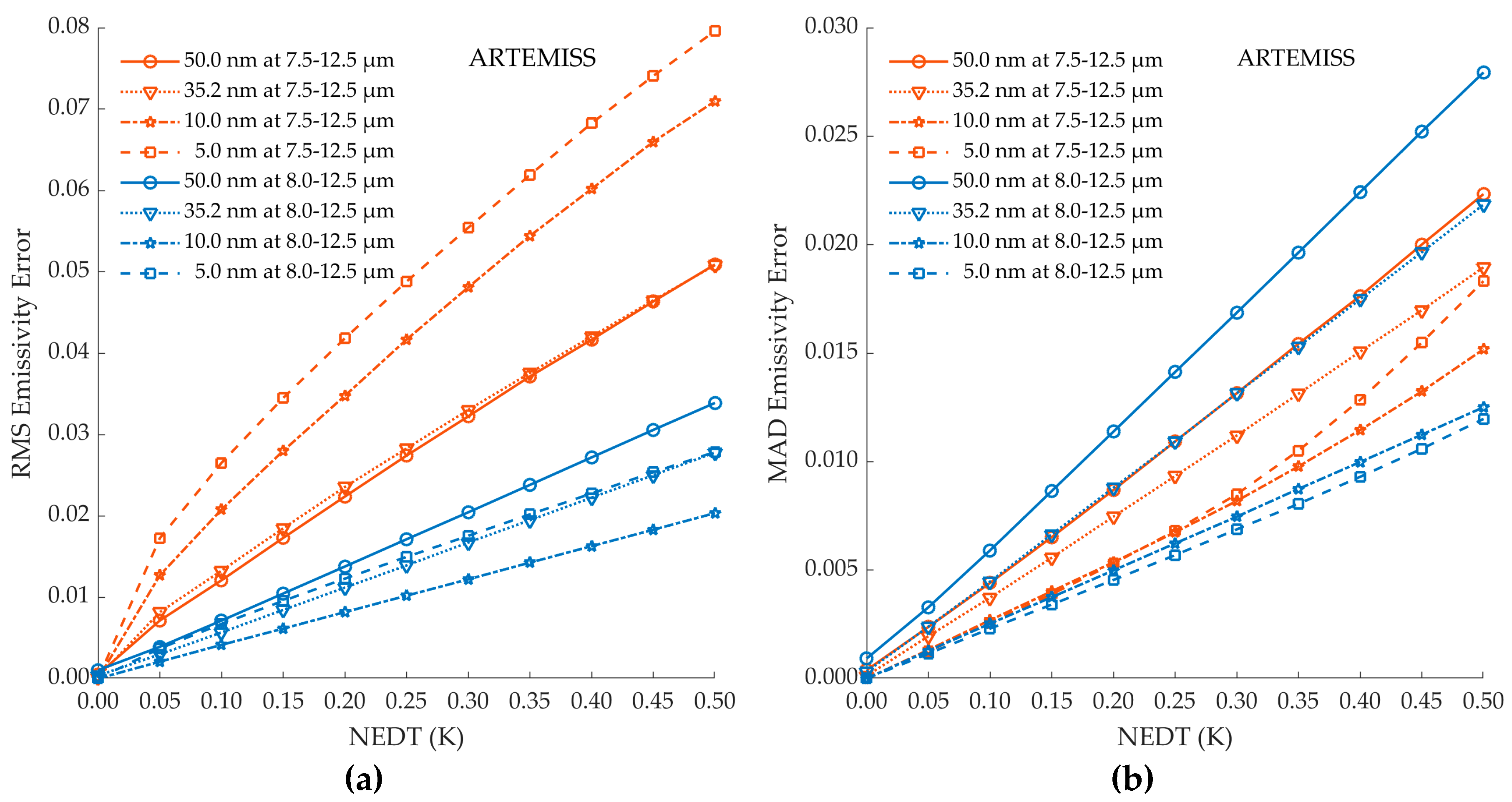
3.2.1. The Relationship of the Retrieval Errors of ARTEMISS vs. the Noise Level and Spectral Parameters

This study retrieved eight groups of simulated HTIR data with two spectral ranges (7.5–12.5 μm and 8–12.5 μm) and four spectral resolution (50 nm, 35.2 nm, 10 nm and 5 nm) by the ARTEMISS algorithm and measured the retrieved LST and LSE errors. Figure 1 shows the retrieved LST errors of the eight groups of simulated HTIR data as a function of the noise level.

For all eight groups of simulated HTIR data shown in Figure 1, the retrieved LST errors of ARTEMISS increased linearly, roughly with the noise level. For the four groups of simulated data with high spectral resolution of 10 nm and 5 nm, after the NEDT of 0.2 K, the retrieved LST errors increased with the noise level at a slower growth rate. For the eight groups of simulated data except the two with the spectral resolution of 5 nm, the retrieved LST errors of ARTEMISS decreased as the spectral resolution increased. However, the two groups of data with a spectral resolution of 5 nm show differences to each other. For the spectral range of 8–12.5 μm, the retrieved LST errors of 5 nm at 8–12.5 μm (refers to Group8 with a spectral resolution of 5 nm and in a spectral range of 8–12.5 μm) were smaller than those with a lower spectral resolution (50 nm and 35.2 nm) and were consistent with those of 10 nm and a spectral range of 8–12.5 μm in terms of both amplitude and trend. For the spectral range of 7.5–12.5 μm, the retrieved LST errors of 5 nm at 7.5–12.5 μm were larger than those with a lower spectral resolution (35.2 nm and 10 nm) and were numerically similar with those of 50 nm at 7.5–12.5 μm. For the spectral resolutions of 50 nm and 32.5 nm, the retrieved LST errors with a spectral range of 7.5–12.5 μm were smaller than those in the spectral range of 8–12.5 μm. Among the eight groups of results, the group with 10 nm at 8–12.5 μm had the smallest retrieved LST error (e.g., LST RMSE = 0.11 K, 0.55 K and 1.10 K when NEDT = 0.05 K, 0.20 K and 0.50 K, respectively), 50 nm at 8–12.5 μm had the largest retrieval LST error (e.g., LST RMSE = 0.46 K, 1.20 K and 2.56 K when NEDT = 0.05 K, 0.20 K and 0.50 K, respectively). The results suggest that for temperature inversion, a higher spectral resolution and wider spectral range do not necessarily lead to smaller LST inversion errors. The results of this study show that, considering noise, 10 nm at 8–12.5 μm was the most suitable setting for thermal infrared hyperspectral temperature inversion among the eight spectral settings investigated.

Figure 2a,b shows the RMSE and MAD of ARTEMISS retrieved LSE for eight groups of simulated HTIR data. Figure 2a shows that the retrieved LSE RMSEs of ARTEMISS increased approximately linearly with the noise level for all eight groups of simulated HTIR data, which is consistent with the retrieved LST RMSEs in Figure 1. However, the retrieved LSE RMSEs show a significant difference between the two spectral ranges. The retrieved LSE RMSEs of all four groups of data in the spectral range of 8–12.5 μm were smaller than the retrieved LSE RMSEs of four groups of data with in spectral range of 7.5–12.5 μm. Moreover, the relationship between the retrieved LSE RMSEs and the spectral resolution were different in the two spectral ranges. For the four groups of data in spectral range of 7.5–12.5 μm, the retrieved LSE RMSEs of ARTEMISS increased as the spectral resolution increased; in contrast, for the four groups of data in the spectral range of 8–12.5 μm, the retrieved LSE RMSEs of ARTEMISS decreased as the spectral resolution increased (except the group of 5 nm at 8–12.5 μm). Among the eight groups, 10 nm at 8–12.5 μm had the smallest LSE RMSEs (0.0021, 0.0082 and 0.0203 when NEDT = 0.05 K, 0.20 K and 0.5 K, respectively), while the 5 nm at 7.5–12.5 μm had the largest LSE RMSEs (0.0173, 0.0418 and 0.0796 when NEDT = 0.05 K, 0.20 K and 0.5 K, respectively). Figure 2b shows that the trend of the retrieved LSE MADs of ARTEMISS was close to that of the retrieved LST RMSEs for the eight groups. For the eight groups of data with two spectral ranges, the retrieved LSE MADs of ARTEMISS roughly increased linearly with the noise level. Moreover, the relationship between the retrieved LSE MADs and the spectral resolution were the same for the two spectral ranges. The retrieved LSE MADs decreased as the spectral resolution increased, except for 5 nm at 7.5–12.5 μm. Among the eight groups, 5 nm at 8–12.5 μm had the smallest retrieved LSE MADs and 50 nm at 8–12.5 μm had the largest retrieved LSE MADs.

The LSE RMSE represents the degree to which the retrieved emissivity spectrum deviates from the true value at each band numerically, while LSE MAD represents the degree to which the retrieved emissivity spectrum deviates from the true spectral curve in the overall shape. Figure 1 and Figure 2b show that the smaller the temperature inversion error, the smaller the emissivity MAD, indicating that the more accurate the temperature inversion, the closer the overall trend of the inversion emissivity curve is to the true spectrum curve. Both the retrieved LST errors and the retrieved LSE MADs of the four groups of data with a spectral range of 7.5–12.5 μm are between those of 10 nm at 8–12.5 μm and 50 nm at 8–12.5 μm with a spectral range of 8–12.5 μm. However, the retrieved LSE RMSEs of all four groups of data with a spectral range of 7.5–12.5 μm were larger than those with a spectral range of 8–12.5 μm. The reason for this seemingly contradictory phenomenon is that, compared to 8–12.5 μm, the retrieved LSE spectra with a spectral range of 7.5–12.5 μm (especially 7.5–8.0 μm is where dense atmospheric absorption lines exist) have large outliers in some bands, as shown in Figure 3. The existence of the huge outliers causes the cases that although the retrieved LSE has a large RMSE, the overall shape of the retrieved emissivity is closer to the true curve than some retrieved LSE with a small RMSE. The finding that in terms of the spectral range of 7.5–12.5 μm, the higher the spectral resolution is, the larger the retrieved LSE RMSE, suggests that for the cases with a spectral range of 7.5–12.5 μm, the higher the spectral resolution was, the more outliers of the retrieved LSE RMSE occurred. This also suggests that for thermal infrared hyperspectral remote sensing, the spectral range of 8–12.5 μm is more suitable for temperature inversion, which is similar to the statement in [42].

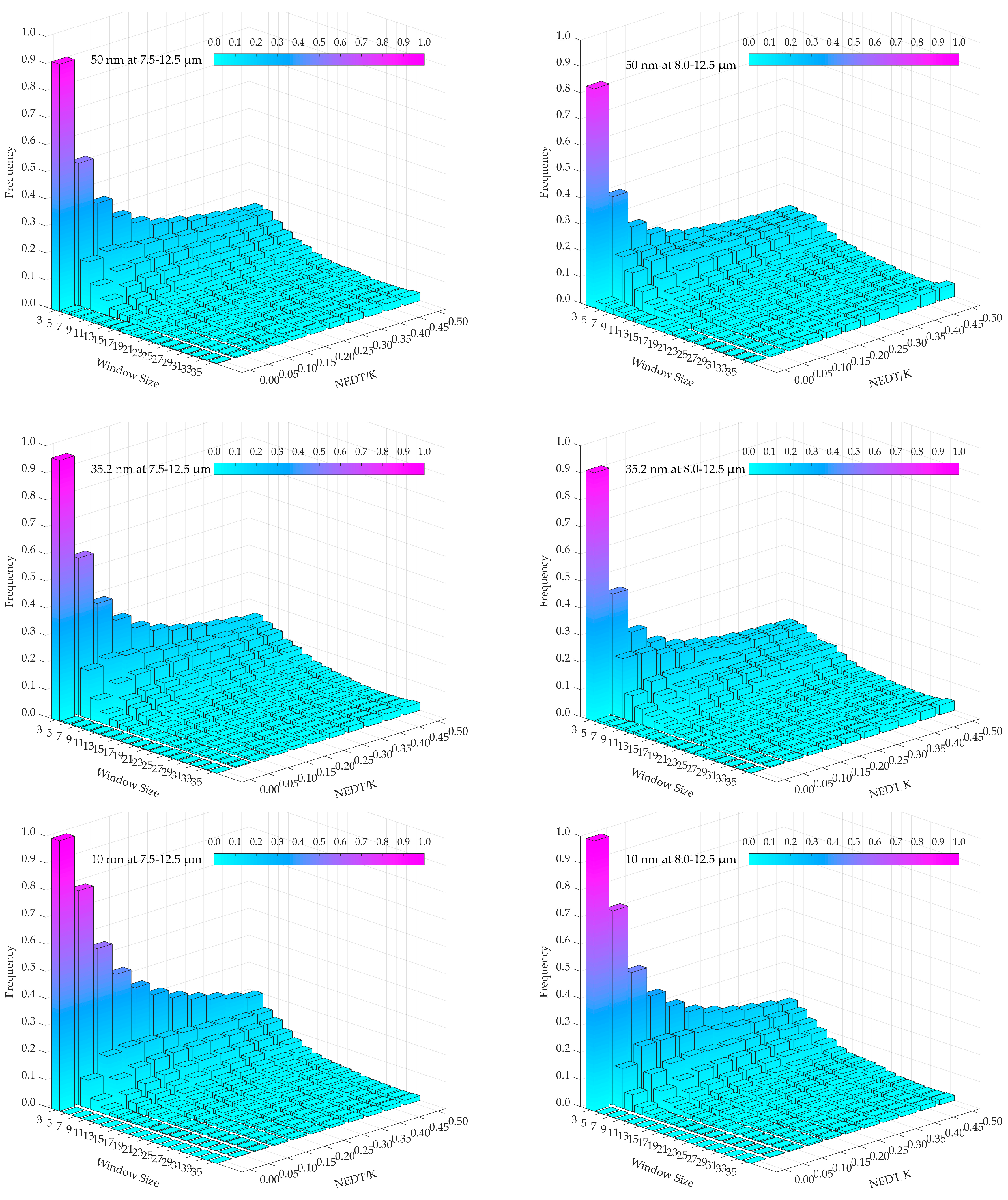
3.2.2. The Relationship of the Retrieval Errors vs. the Optimal Window Size Spectral Smoothing

To investigate the effect of the window size for the spectral smoothing index in ARTEMISS on the retrieved LST and LSE errors, we tested 17 spectral smoothing window sizes for ARTEMISS, going from 3 to 35 in increments of 2 for eight groups of simulated data with two spectral ranges and four spectral resolutions. In the process of a simulated radiance spectrum inversion, we looped the window size for spectral smoothing, calculated the cost functions and found the smallest one among all of the cost functions under 17 window sizes. The temperature at the minimum cost function was considered as the retrieved LST, the corresponding emissivity was the retrieved LSE, and the corresponding window size was the optimal spectral smoothing window size because the retrieved LST error was close to zero in the majority of cases. Figure 4 has eight subplots for the eight groups of simulated data, each of which shows the distribution of the optimal spectral smoothing window size vs. the noise level under a certain spectral setting. The distributions of the optimal spectral smoothing window size vs. the noise level show a consistent trend for the eight spectral settings. For each noise level, the window size with the largest proportion is 3. Generally, the larger the window size, the smaller the proportion (except 35, at the end of the window size range). In the ideal situation without noise, a window size of 3 has the most advantageous proportion in the optimal spectral smoothing window size distribution, especially when the spectral resolution is high (e.g., 10 nm and 5 nm); as the noise level increased, the proportion of the window size 3 gradually decreased for a certain spectral setting. The results suggest that when the hyperspectral thermal infrared data is noisy, it may be beneficial to improve the accuracy of temperature inversion by increasing the spectral smoothing window size in some cases.

4. The Proposal and Validation of the RDSS Algorithm

4.1. RDSS—An Improved TES Algorithm Based on ARTEMISS

The coupling of temperature and emissivity, as shown in Equation (9), suggests that the temperature is easier to determine than the emissivity in the TES process. Therefore, most algorithms adopt the strategy of first determining the temperature and then calculating the emissivity. Hence, accurately determining the temperature has also become the key to TES. We rewrite Equation (9) by combining the items determined by the temperature estimation and the items determined by both the temperature estimation and noise as follows:

$$\sigma \left(\widehat{T},\overline{\widehat{\epsilon }}\right)=\sigma \left(\left(f_{\epsilon }\left({\widehat{B}}_i\right)+f_{\eta }\left({\widehat{B}}_i\right)\right)\left({\widehat{B}}_i-L_i^d\right){\tau }_i-\left(B_i-L_i^d\right){\epsilon }_i{\tau }_i-{\eta }_i\right)$$

(13)

where $f_{\epsilon }\left({\widehat{B}}_i\right)$ and $f_{\eta }\left({\widehat{B}}_i\right)$ are the emissivity estimation after box-average smoothing and the residual containing noise respectively. For the algorithms that use the standard deviation of the simulated at-sensor radiance and the actual at-sensor radiance as the cost function, $f_{\epsilon }\left({\widehat{B}}_i\right)$ and $f_{\eta }\left({\widehat{B}}_i\right)$ can also be considered as the approximately processed emissivity and residual noise, respectively. They can be expressed as

$$f_{\epsilon }\left({\widehat{B}}_i\right)=\frac{B_{i-1}-L_{i-1}^d}{{\widehat{B}}_{i-1}-L_{i-1}^d}\frac{{\epsilon }_{i-1}}{3}+\frac{B_i-L_i^d}{{\widehat{B}}_i-L_i^d}\frac{{\epsilon }_i}{3}+\frac{B_{i+1}-L_{i+1}^d}{{\widehat{B}}_{i+1}-L_{i+1}^d}\frac{{\epsilon }_{i+1}}{3}$$

(14)

$$f_{\eta }\left({\widehat{B}}_i\right)=\frac{1}{3}\frac{\frac{{\eta }_{i-1}}{{\tau }_{i-1}}}{{\widehat{B}}_{i-1}-L_{i-1}^d}+\frac{1}{3}\frac{\frac{{\eta }_i}{{\tau }_i}}{{\widehat{B}}_i-L_i^d}+\frac{1}{3}\frac{\frac{{\eta }_{i+1}}{{\tau }_{i+1}}}{{\widehat{B}}_{i+1}-L_{i+1}^d}$$

(15)

When the emissivity approximation processing can remove the “thorns” in a curve caused by atmospheric background radiation and obtain relatively accurate $f_{\epsilon }\left({\widehat{B}}_i\right)$, and the noise residuals $f_{\eta }\left({\widehat{B}}_i\right)$ with a noise item ${\eta }_i$ of 0 or close to 0, the searched optimal temperature is likely to be equal or much closer to the true temperature. As the magnitude of noise residuals $f_{\eta }\left({\widehat{B}}_i\right)$ and noise term ${\eta }_i$ increase, it is likely that the signs of the items will cancel each other out, resulting in the searched optimal temperature deviating from the true surface temperature. The results of ARTEMISS sensitivity on the spectral smoothing window size in Section 3.2.2 suggest that increasing the spectral smoothing window size did not effectively reduce the inversion error; different window sizes are needed to find the optimal temperature as close to the true one possible when different noises, emissivity and transmittances are coupled together. However, it will add computation complexity and cost much more computation time. That is to say, it is difficult to remove the influence of noise on the optimal temperature search simply by emissivity approximation processing. Therefore, in this study, from the perspective of reducing the noise of the data, we filtered the variables participating in the calculation of the emissivity estimation with a unified filter. The unified filter ensured the variables were at the same spectral resolution while eliminating the noise in the at-sensor radiances. We named the TES algorithm proposed in this study the resolution-degrade-based spectral smoothness (RDSS) algorithm. The calculation process of RDSS is:

(1) Unified filtering: before calculating the emissivity with Equation (4), we filtered each variable participating in the calculation of the emissivity estimation with mean filtering. The calculation method was as follows:

$$\tilde{V}=F\left(V\right)$$

(16)

where $F$ is the filter function, $V$ is the variable to be filtered and $\tilde{V}$ is the filtered variable. Here, the variables refer to the ground-leaving radiance, the atmospheric downwelling radiance and the blackbody radiance.

Specifically, the calculation method for filtering the variables in Equation (4) with a mean filter was as follows:

$$\left[{\tilde{L}}_g\left({\lambda }_i,T\right),{\tilde{L}}_d\left({\lambda }_i\right),\tilde{B}\left({\lambda }_i,\widehat{T}\right)\right]=\frac{1}{2N_r+1}{\displaystyle \sum }_{j=-N_r}^{N_r}\left[L_g\left({\lambda }_{i+j},T\right),L_d\left({\lambda }_{i+j}\right),B\left({\lambda }_{i+j},\widehat{T}\right)\right]$$

(17)

where ${\tilde{L}}_g\left({\lambda }_i,T\right)$, ${\tilde{L}}_d\left({\lambda }_i\right)$ and $\tilde{B}\left({\lambda }_i,\widehat{T}\right)$ are the filtered $L_g\left({\lambda }_{i+j},T\right)$, $L_d\left({\lambda }_{i+j}\right)$ and $B\left({\lambda }_{i+j},\widehat{T}\right)$, respectively, with the mean filter; and $2N_r+1$ is the spectral smoothing window size.

(2) Emissivity estimation and approximate processing: to avoid the local minimum value issue, taking advantage of the fact that the object temperature has a finite value range as a physical parameter, this study adopted the strategy of an exhaustive search to find the optimal temperature. We determined a temperature search range $Tsu{p}_{inf}$ and the incremental step $\delta T$ (also named as the temperature resolution), then calculated the emissivity estimations for all of the temperatures in the search range and approximately processed the emissivity estimations (i.e., boxcar average):

$$\widehat{\epsilon }\left({\lambda }_i,T_{inf}()\frac{{\tilde{L}}_g\left({\lambda }_i,T\right)-{\tilde{L}}_d\left({\lambda }_i\right)}{\tilde{B}({\lambda }_i,T{\widetilde{-}}_d{{}_i}_{inf}}\right)$$

(18)

$$\tilde{\epsilon }\left({\lambda }_i,T_{inf}()\frac{1}{3}{\displaystyle \sum }_{j=-1}^{1\sum }\widehat{\epsilon }\left({\lambda }_{i+j},T_{inf}()\right)\right)$$

(19)

where $\widehat{\epsilon }\left({\lambda }_i,T_{inf}()\right)$ is the emissivity estimation at the temperature of $T_{inf}$, $k$ is the steps, $k=0,1,2,\dots ,\left(T_{\sup }-T_{\inf }\right)/\delta T$ and $\tilde{\epsilon }\left({\lambda }_i,T_{inf}()\right)$ is the corresponding emissivity estimation of $\widehat{\epsilon }\left({\lambda }_i,T_{inf}()\right)$ after approximate processing.

(3) Cost function calculation and the optimal temperature determination. We calculated the cost functions for all temperatures in the temperature search range according to the approximate processed emissivity. The calculation method was as follows:

$$\sigma \left(T_{\inf }+\delta T\cdot k\right)=\sigma \left(\left(\tilde{B}({\lambda }_i,T_{\inf }+\delta T\cdot k)-{\tilde{L}}_d({\lambda }_i)\right)\tilde{\epsilon }\left({\lambda }_i,T_{\inf }+\delta T\cdot k\right)+{\tilde{L}}_d({\lambda }_i)-{\tilde{L}}_g({\lambda }_i,T)\right)$$

(20)

$$inf\underset{k}{\arg min}\left(\sigma \left(T_{inf}()\right)()\right){\widehat{T}}_{opt}=T$$

(21)

where ${\widehat{T}}_{opt}$ is the optimal temperature estimation, i.e., the retrieved temperature.

(4) Final emissivity calculation: we substituted the retrieved temperature from (3) and the other three variables before filtering them into Equation (4) to obtain the final emissivity. The calculation method was:

$${\widehat{\epsilon }}_{opt}\left({\lambda }_i\right)=\frac{L_g\left({\lambda }_i,T\right)-L_d\left({\lambda }_i\right)}{B\left({\lambda }_i,{\widehat{T}}_{opt}\right)-L_d\left({\lambda }_i\right)}$$

(22)

where ${\widehat{\epsilon }}_{opt}\left({\lambda }_i\right)$ is the final emissivity estimation, i.e., the retrieved emissivity.

4.2. Validation Results Analysis

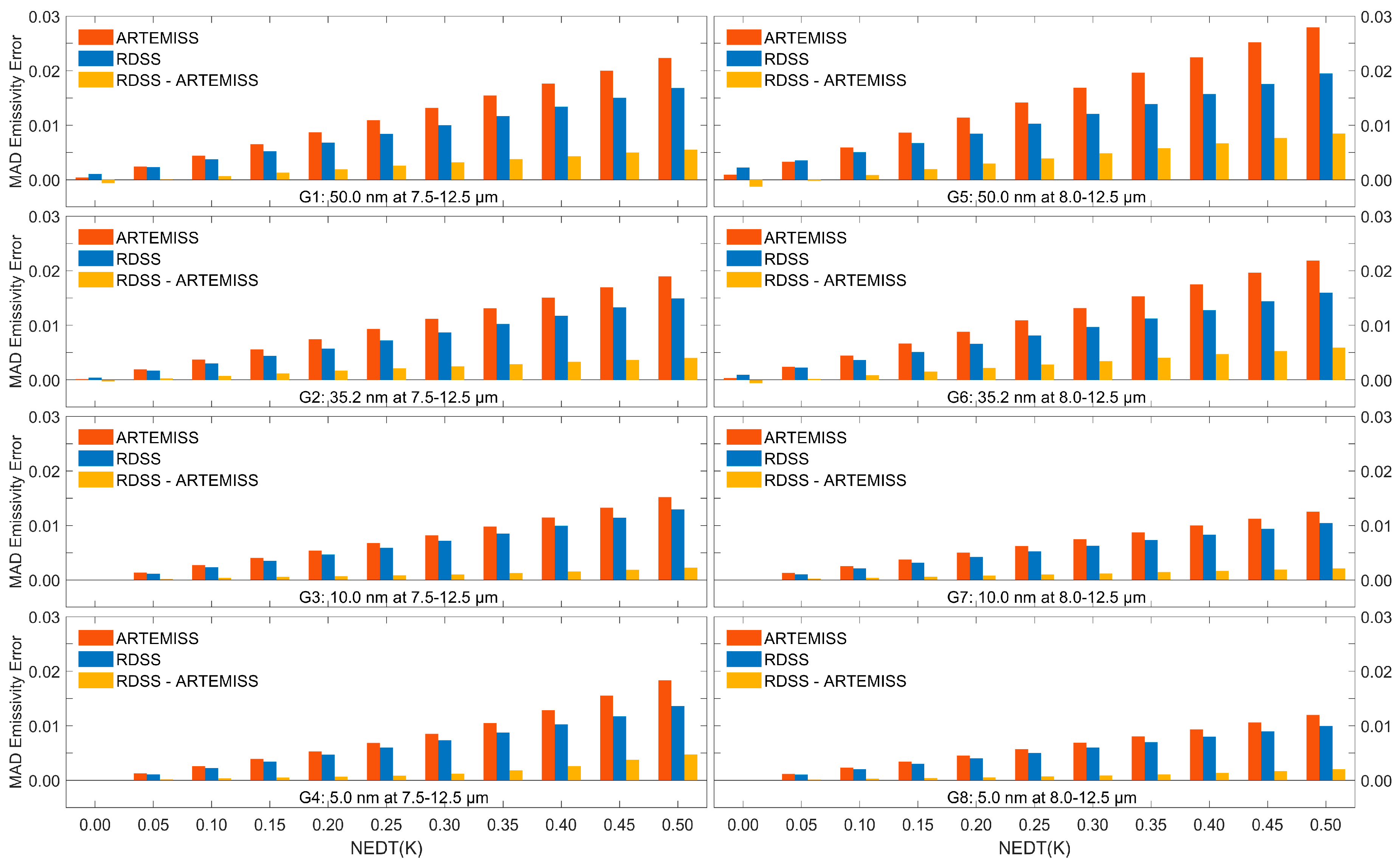
4.2.1. The Retrieval Errors of the RDSS Algorithm

We retrieved the eight groups of simulated HTIR data with two spectral ranges (7.5–12.5 μm and 8–12.5 μm) and four spectral resolutions (50 nm, 35.2 nm, 10 nm and 5 nm) using the RDSS algorithm and measured the retrieved LST and LSE errors. Figure 5 and Figure 6 show the retrieved LST errors and the retrieved LSE errors of the eight groups of simulated HTIR data as a function of the noise level, respectively. The change trends of the retrieved LST and LSE errors of the RDSS algorithm with noise, spectral resolution and spectral range were basically the same as those of the ARTEMISS algorithm, namely both the LST and LSE errors increase with noise linearly. The difference is that in terms of the magnitude of errors, the LST and LSE errors of RDSS were smaller than those of ARTEMISS except for some LSE RMSEs.

Figure 7 shows a comparison chart of RDSS and ARTEMISS on the retrieved LST error, and

Table 3. The retrieved LST error list of the RDSS and ARTEMISS and their differences.

Groups\NEDT(K)		0.00	0.05	0.10	0.15	0.20	0.25	0.30	0.35	0.40	0.45	0.50
G1 1	A 2	0.14	0.30	0.51	0.78	0.99	1.22	1.45	1.65	1.84	2.05	2.22
	R 3	0.44	0.48	0.58	0.70	0.84	0.96	1.09	1.25	1.38	1.50	1.66
	Dif 4	−0.30	−0.18	−0.07	0.08	0.15	0.26	0.36	0.40	0.46	0.55	0.56
	RDif 5	—	—	—	10%	15%	21%	25%	24%	25%	27%	25%
G2	A	0.05	0.21	0.42	0.62	0.84	1.02	1.20	1.41	1.56	1.73	1.89
	R	0.13	0.20	0.32	0.46	0.59	0.72	0.85	1.00	1.11	1.22	1.34
	Dif	−0.08	0.01	0.10	0.16	0.24	0.31	0.35	0.41	0.45	0.51	0.55
	RDif	—	5%	24%	26%	29%	30%	29%	29%	29%	29%	29%
G3	A	0.00	0.19	0.39	0.61	0.80	0.94	1.11	1.27	1.44	1.60	1.77
	R	0.01	0.14	0.29	0.45	0.59	0.71	0.83	0.96	1.08	1.18	1.30
	Dif	0.00	0.05	0.10	0.16	0.21	0.23	0.27	0.31	0.36	0.42	0.48
	RDif	—	26%	26%	26%	26%	24%	24%	24%	25%	26%	27%
G4	A	0.00	0.25	0.54	0.77	0.98	1.18	1.36	1.59	1.83	2.10	2.34
	R	0.00	0.19	0.39	0.61	0.76	0.91	1.04	1.18	1.31	1.43	1.59
	Dif	0.00	0.06	0.15	0.17	0.22	0.27	0.33	0.41	0.52	0.66	0.75
	RDif	—	24%	28%	22%	22%	23%	24%	26%	28%	31%	32%
G5	A	0.30	0.46	0.69	0.97	1.20	1.46	1.70	1.91	2.14	2.36	2.56
	R	0.89	0.91	0.97	1.05	1.15	1.26	1.39	1.52	1.67	1.76	1.91
	Dif	−0.58	−0.45	−0.28	−0.08	0.04	0.20	0.31	0.39	0.47	0.59	0.65
	RDif	—	—	—	—	3%	14%	18%	20%	22%	25%	25%
G6	A	0.11	0.27	0.48	0.70	0.92	1.13	1.33	1.53	1.69	1.87	2.02
	R	0.27	0.32	0.41	0.53	0.67	0.80	0.92	1.07	1.17	1.30	1.42
	Dif	−0.17	−0.05	0.07	0.17	0.25	0.33	0.41	0.45	0.53	0.57	0.59
	RDif	—	—	15%	24%	27%	29%	31%	29%	31%	30%	29%
G7	A	0.00	0.11	0.24	0.41	0.55	0.64	0.75	0.87	0.97	1.07	1.20
	R	0.01	0.06	0.13	0.20	0.28	0.35	0.43	0.48	0.56	0.62	0.67
	Dif	0.00	0.05	0.11	0.21	0.27	0.29	0.33	0.39	0.41	0.45	0.53
	RDif	—	45%	46%	51%	49%	45%	44%	45%	42%	42%	44%
G8	A	0.00	0.11	0.26	0.45	0.57	0.69	0.78	0.88	0.99	1.11	1.23
	R	0.00	0.06	0.11	0.19	0.26	0.35	0.41	0.50	0.55	0.61	0.67
	Dif	0.00	0.05	0.14	0.26	0.31	0.34	0.37	0.39	0.44	0.50	0.57
	RDif	—	45%	54%	58%	54%	49%	47%	44%	44%	45%	46%

¹ Group 1. ² ARTEMISS. ³ RDSS. ⁴ Difference between RDSS and ARTEMISS (i.e., RDSS – ARTEMISS). ⁵ Relative difference between RDSS and ARTEMISS (RDSS – ARTEMISS)/ARTEMISS). ⁶ The gray values show how much RDSS performs better than ARTEMISS and the bold values are the maximum reduction in error. Figure 8 shows a comparison of RDSS and ARTEMISS on the retrieved LSE RMSEs, and Table 4 is a list of the RMSE corresponding to Figure 8. Figure 9 shows a comparison chart of RDSS and ARTEMISS on the retrieval LSE MADs, and Table 5 is a list of the MAD corresponding to Figure 9. The results of LSE RMSE show that unlike the retrieval LST RMSE, for a few of the eleven noise levels and eight spectral settings (31 of 88 cases), the retrieved LSE RMSEs from the RDSS are smaller than those of the ARTEMISS algorithm. From the perspective of LSE RMSE, it seems that the RDSS had limited improvement on the emissivity inversion accuracy, and was not as good as ARTEMISS in terms of the overall effect. However, the results for LSE MAD tell another story.

shows the corresponding error list. They show that under most noise and spectral settings, the retrieved LST error of RDSS are reduced by varying degrees, with a maximum reduction of 0.75 K (Group4, NDET = 0.5 K). The reduced values of the retrieved LST errors vary for different noise levels and spectral settings. Specifically, the reduced degrees of RDSS LST errors increase with the noise level; however, LST errors of RDSS are larger than ARTEMISS when there are no noise or less noise. The initial noise level at which LST errors of RDSS became smaller than ARTEMISS decreased as the spectral resolution increased. For example, the initial noise level decreased from 0.15 (Group1) and 0.2 K (Group5) with a spectral resolution of 50 nm to 0.05 K and 0.05 K (Group4 and Group8) with the spectral resolution of 5 nm, respectively. The above trends indicate that in terms of temperature inversion, RDSS was more effective for data with high noise levels and a high spectral resolution. The same temperature inversion accuracy can be obtained by RDSS, while the instrument design specifications or data correction accuracy were reduced.

Figure 8 shows a comparison of RDSS and ARTEMISS on the retrieved LSE RMSEs, and

Table 4. The retrieved LSE RMSE for RDSS and ARTEMISS and their differences.

Groups\NEDT(K)		0.00	0.05	0.10	0.15	0.20	0.25	0.30	0.35	0.40	0.45	0.50
G1	A	0.0005	0.0071	0.0121	0.0173	0.0224	0.0274	0.0322	0.0371	0.0417	0.0464	0.0509
	R	0.0016	0.0140	0.0248	0.0343	0.0423	0.0506	0.0592	0.0685	0.0772	0.0888	0.0954
	Dif	−0.0011	−0.0068	−0.0127	−0.0171	−0.0199	−0.0232	−0.0270	−0.0314	−0.0355	−0.0425	−0.0445
	RDif	—	—	—	—	—	—	—	—	—	—	—
G2	A	0.0002	0.0082	0.0133	0.0185	0.0235	0.0283	0.0330	0.0376	0.0420	0.0465	0.0508
	R	0.0006	0.0138	0.0254	0.0358	0.0468	0.0576	0.0705	0.0843	0.0982	0.1107	0.1203
	Dif	−0.0004	−0.0056	−0.0121	−0.0174	−0.0233	−0.0293	−0.0374	−0.0467	−0.0562	−0.0642	−0.0695
	RDif	—	—	—	—	—	—	—	—	—	—	—
G3	A	0.0000	0.0127	0.0208	0.0280	0.0348	0.0417	0.0481	0.0544	0.0602	0.0660	0.0710
	R	0.0000	0.0192	0.0416	0.0735	0.1081	0.1576	0.1927	0.2392	0.2591	0.2950	0.3037
	Dif	0.0000	−0.0065	−0.0208	−0.0455	−0.0733	−0.1159	−0.1446	−0.1848	−0.1989	−0.2290	−0.2327
	RDif	—	—	—	—	—	—	—	—	—	—	—
G4	A	0.0000	0.0172	0.0265	0.0345	0.0418	0.0488	0.0554	0.0619	0.0683	0.0741	0.0796
	R	0.0000	0.0095	0.0252	0.0427	0.0565	0.0720	0.0831	0.0994	0.1082	0.1221	0.1318
	Dif	0.0000	0.0078	0.0013	−0.0082	−0.0147	−0.0232	−0.0277	−0.0375	−0.0399	−0.0480	−0.0522
	RDif	—	45%	5%	—	—	—	—	—	—	—	—
G5	A	0.0010	0.0039	0.0071	0.0104	0.0138	0.0171	0.0204	0.0238	0.0272	0.0306	0.0339
	R	0.0026	0.0042	0.0063	0.0085	0.0108	0.0131	0.0155	0.0179	0.0203	0.0226	0.0251
	Dif	−0.0015	−0.0003	0.0008	0.0019	0.0030	0.0040	0.0050	0.0059	0.0069	0.0079	0.0088
	RDif	—	—	11%	18%	22%	23%	25%	25%	25%	26%	26%
G6	A	0.0004	0.0030	0.0057	0.0084	0.0112	0.0139	0.0167	0.0195	0.0222	0.0250	0.0278
	R	0.0011	0.0028	0.0048	0.0068	0.0089	0.0110	0.0132	0.0153	0.0174	0.0196	0.0217
	Dif	−0.0007	0.0001	0.0009	0.0016	0.0023	0.0029	0.0036	0.0042	0.0049	0.0054	0.0061
	RDif	—	3%	16%	19%	21%	21%	22%	22%	22%	22%	22%
G7	A	0.0000	0.0021	0.0041	0.0061	0.0082	0.0102	0.0122	0.0143	0.0163	0.0183	0.0203
	R	0.0000	0.0018	0.0038	0.0057	0.0076	0.0095	0.0115	0.0134	0.0156	0.0175	0.0198
	Dif	0.0000	0.0002	0.0004	0.0005	0.0006	0.0007	0.0007	0.0008	0.0007	0.0008	0.0005
	RDif	—	10%	10%	8%	7%	7%	6%	6%	4%	4%	2%
G8	A	0.0000	0.0037	0.0067	0.0095	0.0123	0.0150	0.0175	0.0202	0.0227	0.0254	0.0278
	R	0.0000	0.0061	0.0128	0.0216	0.0308	0.0399	0.0483	0.0560	0.0635	0.0706	0.0778
	Dif	0.0000	−0.0024	−0.0061	−0.0120	−0.0185	−0.0249	−0.0307	−0.0359	−0.0407	−0.0453	−0.0500
	RDif	—	—	—	—	—	—	—	—	—	—	—

is a list of the RMSE corresponding to Figure 8. Figure 9 shows a comparison chart of RDSS and ARTEMISS on the retrieval LSE MADs, and

Table 5. The retrieved LSE MAD for the RDSS and ARTEMISS algorithms and their differences.

Groups\NEDT(K)		0.00	0.05	0.10	0.15	0.20	0.25	0.30	0.35	0.40	0.45	0.50
G1	A	0.0004	0.0024	0.0044	0.0065	0.0087	0.0109	0.0131	0.0154	0.0176	0.0200	0.0223
	R	0.0010	0.0023	0.0037	0.0052	0.0068	0.0084	0.0100	0.0116	0.0134	0.0150	0.0168
	Dif	−0.0006	0.0001	0.0007	0.0013	0.0019	0.0026	0.0032	0.0038	0.0043	0.0050	0.0055
	RDif	—	4%	16%	20%	22%	24%	24%	25%	24%	25%	25%
G2	A	0.0001	0.0020	0.0037	0.0056	0.0075	0.0093	0.0112	0.0131	0.0151	0.0170	0.0190
	R	0.0004	0.0017	0.0030	0.0044	0.0058	0.0072	0.0087	0.0102	0.0117	0.0133	0.0149
	Dif	−0.0003	0.0003	0.0007	0.0012	0.0017	0.0021	0.0025	0.0029	0.0033	0.0037	0.0041
	RDif	—	15%	19%	21%	23%	23%	22%	22%	22%	22%	22%
G3	A	0.0000	0.0013	0.0027	0.0040	0.0054	0.0067	0.0082	0.0098	0.0115	0.0132	0.0152
	R	0.0000	0.0011	0.0023	0.0035	0.0047	0.0059	0.0072	0.0085	0.0099	0.0114	0.0129
	Dif	0.0000	0.0002	0.0004	0.0005	0.0007	0.0009	0.0010	0.0013	0.0015	0.0019	0.0022
	RDif	—	15%	15%	13%	13%	13%	12%	13%	13%	14%	14%
G4	A	0.0000	0.0013	0.0026	0.0039	0.0053	0.0068	0.0085	0.0105	0.0128	0.0155	0.0183
	R	0.0000	0.0011	0.0022	0.0034	0.0047	0.0060	0.0073	0.0087	0.0102	0.0117	0.0136
	Dif	0.0000	0.0002	0.0003	0.0005	0.0006	0.0008	0.0012	0.0018	0.0026	0.0038	0.0047
	RDif	—	15%	12%	13%	11%	12%	14%	17%	20%	25%	26%
G5	A	0.0009	0.0033	0.0059	0.0086	0.0114	0.0141	0.0169	0.0196	0.0224	0.0252	0.0279
	R	0.0022	0.0035	0.0050	0.0067	0.0084	0.0102	0.0120	0.0139	0.0157	0.0175	0.0195
	Dif	−0.0013	−0.0002	0.0009	0.0019	0.0029	0.0039	0.0048	0.0058	0.0067	0.0077	0.0085
	RDif	—	—	15%	22%	25%	28%	28%	30%	30%	31%	30%
G6	A	0.0003	0.0024	0.0045	0.0066	0.0088	0.0109	0.0132	0.0153	0.0175	0.0197	0.0218
	R	0.0010	0.0022	0.0036	0.0051	0.0066	0.0081	0.0097	0.0112	0.0128	0.0144	0.0160
	Dif	−0.0006	0.0002	0.0009	0.0015	0.0022	0.0028	0.0035	0.0041	0.0047	0.0053	0.0059
	RDif	—	8%	20%	23%	25%	26%	27%	27%	27%	27%	27%
G7	A	0.0000	0.0013	0.0025	0.0038	0.0050	0.0062	0.0075	0.0087	0.0100	0.0112	0.0125
	R	0.0000	0.0010	0.0021	0.0032	0.0042	0.0052	0.0063	0.0073	0.0083	0.0094	0.0104
	Dif	0.0000	0.0002	0.0004	0.0006	0.0008	0.0010	0.0012	0.0014	0.0017	0.0019	0.0021
	RDif	—	15%	16%	16%	16%	16%	16%	16%	17%	17%	17%
G8	A	0.0000	0.0011	0.0023	0.0034	0.0045	0.0057	0.0069	0.0081	0.0093	0.0106	0.0120
	R	0.0000	0.0010	0.0020	0.0030	0.0040	0.0050	0.0060	0.0070	0.0080	0.0090	0.0100
	Dif	0.0000	0.0001	0.0003	0.0004	0.0005	0.0007	0.0009	0.0011	0.0013	0.0016	0.0020
	RDif	—	9%	13%	12%	11%	12%	13%	14%	14%	15%	17%

is a list of the MAD corresponding to Figure 9. The results of LSE RMSE show that unlike the retrieval LST RMSE, for a few of the eleven noise levels and eight spectral settings (31 of 88 cases), the retrieved LSE RMSEs from the RDSS are smaller than those of the ARTEMISS algorithm. From the perspective of LSE RMSE, it seems that the RDSS had limited improvement on the emissivity inversion accuracy, and was not as good as ARTEMISS in terms of the overall effect. However, the results for LSE MAD tell another story.

Figure 9 and Table 5 show that the retrieved LSE MADs of RDSS have similar distribution with the retrieved LST RMSE for the eight groups of data. For the majority of cases (79 out of 88 cases), the retrieved LSE MADs of RDSS were smaller than those of ARTEMISS. The results of LSE RMSE and LSE MAD behaved differently, probably due to the RMSE itself. The RMSE of an emissivity will be much larger because of some large abnormal values, although the retrieved temperature was accurate. As shown in Figure 10, there were some cases where the retrieved LSE of RDSS with a small LST error and LSE MAD was much closer to the true value from the perspective of the trend of the emissivity curve; however, the RMSE of the emissivity calculated using the accurate temperature was relatively large due to the influence of individual outliers. The phenomenon that the RMSE of an emissivity did not decrease but increased when the retrieved temperature was more accurate was also described in another paper [34].

This study used MAD to evaluate the retrieved LSE error to measure the quality of the retrieved LSE curve from the perspective of the overall degree of deviation of emissivity from the true value. However, MAD cannot be compared with RMSE in terms of values, because MAD focuses on the deviation degree of the overall trend, which is different from the commonly used RMSE in terms of magnitude. We used the percentage of MAD to measure the reduction of the retrieved LSE error, as an indicator reflecting how close the trend of the emissivity curve retrieved by RDSS was to the true emissivity curve. Table 5 shows that the maximum relative decline in the percentage of LSE MAD can reach 31% (G5, 0.45 K). As the noise increased, the decline in the percentage of the LSE MAD of RDSS increased accordingly. When there was no noise or less noise, however, the MAD of RDSS instead increased. This is similar to the retrieved LST error in terms of change characteristics. However, the decline in the percentage of MAD of RDSS did not increase with the spectral resolution. In the range of 7.5–12.5 μm (G1–G4), the decline in the percentage of retrieval LSE MAD firstly decreased, and then increased along with the spectral resolution (it reached a minimum when the spectral resolution was 10 nm); in the range of 8.5–12.5 μm (G5−G8), the decline in the percentage of retrieved LSE MAD gradually decreased as spectral resolution increased. Overall, when the noise level was greater than 0.1 K, the decline in the percentage of the retrieved LSE MAD of RDSS was greater than 10%, which proved the effectiveness of the RDSS algorithm.

4.2.2. The Relationship of RDSS and the Window Setting

During spectral degradation, the window setting ($2N_r+1$ in Equation (17)) is a key parameter. Different window settings may lead to different results, and temperature inversion is the key of the iterative spectral smoothness TES algorithms. The results of this study, at least the LSE MAD results, suggest that the improvement of temperature inversion accuracy is beneficial to the improvement of emissivity inversion accuracy. Therefore, we set 17 spectral smoothing window sizes, ranging from 3 increasing incrementally by 2–35, and separated the temperature and emissivity of the eight sets of simulated data to study the effect of window size on the performance of RDSS. First, we performed a mean filter cyclically with a window size on a radiance curve to obtain spectral degraded radiance curves under different window settings; second, we retrieved the temperatures under different window settings by RDSS, and looped the two steps for the eight groups of data; finally, we measured the retrieved temperature errors under different window settings.

Figure 11 shows the retrieved LST errors for the RDSS algorithm varying with 11 noise levels under 17 window settings for the eight groups of data. For the four groups of data with lower spectral resolutions (G1–2 and G5–6), 3 was the optimal window setting using RDSS, where the retrieved LST errors were the lowest among the 17 window settings under all or most noise levels. For the four groups of data with higher spectral resolutions (G3–4 and G7–8), the optimal window setting increased rapidly with the noise level. For the two groups of data with a spectral range of 7.5–12.5 μm (G3 and G4), the optimal window setting tended to be stable when the noise level was above 0.15 K, i.e., 27 for G3 and 31 for G4. For the group of data in the spectral range of 8–12.5 μm and the spectral resolution of 10 nm (G7), the optimal window setting tended to be stable at a noise level above 0.25 K—5 for G7. For the group of data in a spectral range of 8–12.5 μm and with a spectral resolution of 5 nm (G8), the optimal window setting was not stable but fluctuated in the range 5–21 when the noise level was above 0.05 K. It is worth noting that for the cases in G8 (5 nm at 8–12.5 μm), as the noise increased, the retrieved LST errors corresponding to the optimal window setting and the second optimal one, or even some other window settings, were very close to each other, and their difference was within 0.01 K. Therefore, it can be considered that when separating the LST and LSE with RDSS for HTIR data, we obtained the minimum LST error with a window setting of 3 for HTIR data with a spectral resolution in the tens of nanometers, and need to increase the window setting according to the spectral range and spectral resolution for HTIR data with a spectral resolution of 10 nm.

5. Discussion

This study focused on the sensitivity of an iterative spectral smoothness TES algorithm to the spectral range, spectral resolution, noise and smooth window size. We analyzed the characteristics of the influence of the four variables on temperature and emissivity inversion accuracy, and proposed an improved algorithm called RDSS. Compared with previous studies, this study analyzed the influence of the key spectrometer indices on the inversion error more comprehensively, especially the spectral resolution and the smooth window size.

The improved method, RDSS, performs spectral degradation on the input data, which can eliminate the effect of random noise on the search for the optimal temperature and improve the accuracy of temperature and emissivity inversion. In terms of method validation, the effect of random noise on RDSS was mainly studied in this study, while the effect of atmospheric error on RDSS needs further study. However, RDSS can also further improve the inversion accuracy by effectively removing random noise in atmospheric correction errors. For the systematic errors in atmospheric correction, the performance of the RDSS algorithm is similar to the ARTEMISS algorithm.

The results of this study also provide a valuable reference for the performance improvement of hyperspectral thermal infrared instruments and data processing. The improvement in spectral resolution is beneficial to reducing the error of temperature inversion. However, for a HTIR imager, the spectral resolution is dependent on the spatial resolution. In other words, the spatial resolution may decrease while the spectral resolution is improved, which will lead to the increase of mixed pixels. Without a good pixel decomposition algorithm, the accuracy of TES may decrease. Therefore, it is not a case of “the higher the spectral resolution, the better”. The choice of spectral resolution needs to consider the application requirements, inversion algorithm, instrument design and other factors, and seek the optimal solution. This may be a very meaningful research topic.

From the perspective of the coupling of temperature and emissivity, accurately determining the temperature is an extremely critical step in the TES process. It is naturally believed that the improvement on the accuracy of temperature inversion will bring corresponding improvements in the accuracy of emissivity inversion. However, there are some anomalies that when the retrieval LST error is reduced to a certain value, the RMSE of retrieved LSE increases instead of decreasing. The emissivity of an object is a spectral curve composed of a set of digits, and the evaluation of the retrieval LSE error is equivalent to the measurement of the relationship between the two sets of digits, i.e., the retrieved LSE and the true value. The temperature of an object, however, is a unique value. Therefore, there is a certain difference between the retrieved LSE errors and the retrieved LST errors on the evaluation method. Moreover, the emissivity retrieved from the HTIR data is mostly used for target identification or surface parameters inversion. We adopted MAD alongside RMSE by combining the evaluation index and the application target in the evaluation of the retrieved LSE. In addition, the retrieved LSEs were not denoised before accuracy evaluation in the experiment, resulting in the retention of many outliers. In the practical application of HTIR data, however, the retrieved LSE curves can be denoised to eliminate outliers; at this moment, the evaluation of the trend of LSE becomes particularly important. Furthermore, the highest spectral resolution in the simulation experiment of the study was set to 5 nm, which is mainly considering that the spectral resolution of the emissivity of the ground objects in the ASTER spectral library is 10 nm or lower. Therefore, cases with a higher spectral resolution than 5 nm need further research when there are emissivity spectra of ground objects with sufficiently high spectral resolution.

6. Conclusions

We focused on the study of instrument noise, a widely existing factor that is difficult to eliminate losslessly in hyperspectral thermal infrared data, and focused on optimizing instrument design. Taking the ARTEMISS algorithm—the representative of the iterative spectral smoothness TES algorithm family with a good application effect—as the object of study. Supplemented by atmospheric radiation transfer simulation software and emissivity spectral library, we carried out simulation and inversion experiments; studied the relationship between the spectral resolution of the instrument, noise level, the ARTEMISS parameter setting and the inversion error; and proposed an improved method—RDSS—based on the mechanism and law of the influence of noise on the inversion error.

The law of the spectral response range, spectral resolution and noise on the inversion error obtained in this study provide a reference for the future development of airborne and spaceborne thermal infrared hyperspectral imagers and optimize the instrument design. The improved TES algorithm can be used for temperature and emissivity inversion of various thermal infrared hyperspectral remote sensing data. The resistance of this method also provides a certain surplus space for the design of the instrument in NEDT.

References

1. Aslett, Z.; Taranik, J.V.; Riley, D.N. Mapping Rock-forming Minerals at Daylight Pass, Death Valley National Park, California, Using SEBASS Thermal-infrared Hyperspectral Image Data. In Proceedings of the 2008 IEEE International Geoscience and Remote Sensing Symposium, Boston, MA, USA, 7–11 July 2008; IEEE Press: Piscataway, NJ, USA, 2009; pp. 366–369. [Google Scholar]
2. Cui, J.; Yan, B.; Dong, X.; Zhang, S.; Zhang, J.; Tian, F.; Wang, R. Temperature and emissivity separation and mineral mapping based on airborne TASI hyperspectral thermal infrared data. Int. J. Appl. Earth Obs. Geoinf. 2015, 40, 19–28. [Google Scholar] [CrossRef]
3. Vaughan, R.G.; Calvin, W.M.; Taranik, J.V. SEBASS hyperspectral thermal infrared data: Surface emissivity measurement and mineral mapping. Remote Sens. Environ. 2003, 85, 48–63. [Google Scholar] [CrossRef]
4. Johnson, W.; Hulley, G.; Hook, S. Remote gas plume sensing and imaging with NASA’s Hyperspectral Thermal Emission Spectrometer (HyTES). In Proceedings of the SPIE Sensing Technology + Applications, Baltimore, MA, USA, 28 May 2014; pp. 91010V-1–91010V-7. [Google Scholar]
5. Palombo, A.; Pascucci, S.; Loperte, A.; Lettino, A.; Castaldi, F.; Muolo, M.R.; Santini, F. Soil Moisture Retrieval by Integrating TASI-600 Airborne Thermal Data, WorldView 2 Satellite Data and Field Measurements: Petacciato Case Study. Sensors 2019, 19, 1515. [Google Scholar] [CrossRef] [Green Version]
6. Guo, G.; Liu, B.; Liu, C. Thermal Infrared Spectral Characteristics of Bunker Fuel Oil to Determine Oil-Film Thickness and API. J. Mar. Sci. Eng. 2020, 8, 135. [Google Scholar] [CrossRef] [Green Version]
7. Wan, Z.; Dozier, J. A generalized split-window algorithm for retrieving land-surface temperature from space. IEEE Trans. Geosci. Remote Sens. 1996, 34, 892–905. [Google Scholar] [CrossRef] [Green Version]
8. Barducci, A.; Pippi, I. Temperature and Emissivity Retrieval from remotely sensed images using the “grey body emissivity” method. IEEE Trans. Geosci. Remote Sens. 1996, 34, 681–695. [Google Scholar] [CrossRef]
9. Kahle, A.B.; Madura, D.P.; Soha, J.M. Middle infrared multispectral aircraft scanner data: Analysis for geological applications. Appl. Opt. 1980, 19, 2279–2290. [Google Scholar] [CrossRef]
10. Gillespie, A.R. Lithologic mapping of silicate rocks using TIMS. In Proceedings of the TIMS Data Users’ Workshop, Pasadena, CA, USA, 18–19 June 1985; pp. 29–44. [Google Scholar]
11. Realmuto, V.J. Separating the effects of temperature and emissivity: Emissivity spectrum normalization. In Proceedings of the Second Thermal Infrared Multispectral Scanner (TIMS) Workshop, Pasadena, CA, USA, 22 May 1991; pp. 31–35. [Google Scholar]
12. Becker, F.; Li, Z.-L. Temperature-independent spectral indices in thermal infrared bands. Remote Sens. Environ. 1990, 32, 17–33. [Google Scholar] [CrossRef]
13. Watson, K. Spectral ratio method for measuring emissivity. Remote Sens. Environ. 1992, 42, 113–116. [Google Scholar] [CrossRef]
14. De Griend, A.A.V.; Owe, M. On the relationship between thermal emissivity and the normalized difference vegetation index for natural surfaces. Int. J. Remote Sens. 1993, 14, 1119–1131. [Google Scholar] [CrossRef]
15. Valor, E.; Caselles, V. Mapping land surface emissivity from NDVI: Application to European, African, and South American areas. Remote Sens. Environ. 1996, 57, 167–184. [Google Scholar] [CrossRef]
16. Sobrino, J.A.; Raissouni, N. Toward remote sensing methods for land cover dynamic monitoring: Application to Morocco. Int. J. Remote Sens. 2000, 21, 353–366. [Google Scholar] [CrossRef]
17. Sobrino, J.A.; Raissouni, N.; Li, Z.-L. A Comparative Study of Land Surface Emissivity Retrieval from NOAA Data. Remote Sens. Environ. 2001, 75, 256–266. [Google Scholar] [CrossRef]
18. Abrams, M. The Advanced Spaceborne Thermal Emission and Reflection Radiometer (ASTER): Data products for the high spatial resolution imager on NASA’s Terra platform. Int. J. Remote Sens. 2000, 21, 847–859. [Google Scholar] [CrossRef]
19. Li, Z.-L.; Wu, H.; Wang, N.; Qiu, S.; Sobrino, J.A.; Wan, Z.; Tang, B.-H.; Yan, G. Land surface emissivity retrieval from satellite data. Int. J. Remote Sens. 2013, 34, 3084–3127. [Google Scholar] [CrossRef]
20. Salisbury, J.W.; D’Aria, D.M. Emissivity of terrestrial materials in the 8–14 μm atmospheric window. Remote Sens. Environ. 1992, 42, 83–106. [Google Scholar] [CrossRef]
21. Borel, C. Iterative Retrieval of Surface Emissivity and Temperature for a Hyperspectral Sensor. In Proceedings of the First JPL Workshop on Remote Sensing of Land Surface Emissivity, Pasadena, CA, USA, 6–8 May 1997. [Google Scholar]
22. Borel, C.C. ARTEMISS–an algorithm to retrieve temperature and emissivity from hyper-spectral thermal image data. In Proceedings of the 28th Annual GOMACTech Conference, Hyperspectral Imaging Session, Tampa, FL, USA, 31 March–3 April 2003; pp. 1–4. [Google Scholar]
23. Borel, C.; Rosario, D.; Romano, J. Data processing and temperature-emissivity separation for tower-based imaging Fourier transform spectrometer data. Int. J. Remote Sens. 2015, 36, 4779–4792. [Google Scholar] [CrossRef]
24. Kanani, K.; Poutier, L.; Nerry, F.; Stoll, M.-P. Directional Effects Consideration to Improve out-doors Emissivity Retrieval in the 3–13 µm Domain. Opt. Express 2007, 15, 12464–12482. [Google Scholar] [CrossRef]
25. Wang, X.; OuYang, X.; Tang, B.; Li, Z.; Zhang, R. A New Method for Temperature/Emissivity Separation from Hyperspectral Thermal Infrared Data. In Proceedings of the IGARSS 2008—2008 IEEE International Geoscience and Remote Sensing Symposium, Boston, MA, USA, 7–11 July 2008; pp. 286–289. [Google Scholar]
26. Cheng, J.; Liu, Q.; Li, X.; Xiao, Q.; Liu, Q.; Du, Y. Correlation-based temperature and emissivity separation algorithm. Sci. China Ser. D Earth Sci. 2008, 51, 357–369. [Google Scholar] [CrossRef]
27. Cheng, J.; Liang, S.; Wang, J.; Li, X. A Stepwise Refining Algorithm of Temperature and Emissivity Separation for Hyperspectral Thermal Infrared Data. IEEE Trans. Geosci. Remote Sens. 2010, 48, 1588–1597. [Google Scholar] [CrossRef]
28. Zhao, H.; Li, J.; Jia, G.; Qiu, X. Correlation-wavelet method for separation of hyperspectral thermal infrared temperature and emissivity. Opt. Precis. Eng. 2019, 27, 1737–1744. [Google Scholar] [CrossRef]
29. Chen, M.; Jiang, X.; Wu, H.; Qian, Y.; Wang, N. Temperature and emissivity retrieval from low-emissivity materials using hyperspectral thermal infrared data. Int. J. Remote Sens. 2019, 40, 1655–1671. [Google Scholar] [CrossRef]
30. Wang, N.; Wu, H.; Nerry, F.; Li, C.; Li, Z. Temperature and Emissivity Retrievals From Hyperspectral Thermal Infrared Data Using Linear Spectral Emissivity Constraint. IEEE Trans. Geosci. Remote Sens. 2011, 49, 1291–1303. [Google Scholar] [CrossRef]
31. Ni, L.; Wu, H.; Zhang, B.; Zhang, W.; Gao, L. Improvement of linear spectral emissivity constraint method for temperature and emissivity separation of hyperspectral thermal infrared data. In Proceedings of the 2015 7th Workshop on Hyperspectral Image and Signal Processing: Evolution in Remote Sensing (WHISPERS), Tokyo, Japan, 2–5 June 2015; pp. 1–4. [Google Scholar]
32. Lan, X.; Zhao, E.; Li, Z.-L.; Labed, J.; Nerry, F. An Improved Linear Spectral Emissivity Constraint Method for Temperature and Emissivity Separation Using Hyperspectral Thermal Infrared Data. Sensors 2019, 19, 5552. [Google Scholar] [CrossRef] [Green Version]
33. Zhang, Y.-Z.; Wu, H.; Jiang, X.-G.; Jiang, Y.-Z.; Liu, Z.-X.; Nerry, F. Land Surface Temperature and Emissivity Retrieval from Field-Measured Hyperspectral Thermal Infrared Data Using Wavelet Transform. Remote Sens. 2017, 9, 454. [Google Scholar] [CrossRef] [Green Version]
34. Zhou, S.; Cheng, J. A multi-scale wavelet-based temperature and emissivity separation algorithm for hyperspectral thermal infrared data. Int. J. Remote Sens. 2018, 39, 8092–8112. [Google Scholar] [CrossRef]
35. Acito, N.; Diani, M.; Corsini, G. Dictionary Based Temperature and Emissivity Separation Algorithm in LWIR Hyperspectral Data. In Proceedings of the 2018 9th Workshop on Hyperspectral Image and Signal Processing: Evolution in Remote Sensing (WHISPERS), Amsterdam, Netherlands, 23–26 September 2018; pp. 1–5. [Google Scholar]
36. Acito, N.; Diani, M.; Corsini, G. Subspace-Based Temperature and Emissivity Separation Algorithms in LWIR Hyperspectral Data. IEEE Trans. Geosci. Remote Sens. 2019, 57, 1523–1537. [Google Scholar] [CrossRef]
37. Ingram, P.M.; Muse, A.H. Sensitivity of iterative spectrally smooth temperature/emissivity separation to algorithmic assumptions and measurement noise. IEEE Trans. Geosci. Remote Sens. 2001, 39, 2158–2167. [Google Scholar] [CrossRef]
38. Cheng, J.; Xiao, Q.; Liu, Q.; Li, X. Effects of Smoothness Index on the Accuracy of Iterative Spectrally Smooth Temperature/Emissivity Separation Algorithm. J. Atmos. Environ. Opt. 2007, 2, 376–380. [Google Scholar]
39. Cheng, J.; Du, Y.; Liu, Q.; Li, X.; Xiao, Q.; Liu, Q. Analysis of the Non-isothermal Effects on the Temperature/Emissvity Separation of Flat Mixed Pixel. J. Atmos. Environ. Opt. 2008, 3, 57–64. [Google Scholar]
40. Borel, C. Error analysis for a temperature and emissivity retrieval algorithm for hyperspectral imaging data. Int. J. Remote Sens. 2008, 29, 5029–5045. [Google Scholar] [CrossRef]
41. OuYang, X.; Wang, N.; Wu, H.; Li, Z.-L. Errors analysis on temperature and emissivity determination from hyperspectral thermal infrared data. Opt. Express 2010, 18, 544–550. [Google Scholar] [CrossRef]
42. Borel, C.C. Temperature-Emissivity Separation Algorithms for Hyperspectral Imaging Spectrometers. In Proceedings of the Fourier Transform Spectroscopy and Hyperspectral Imaging and Sounding of the Environment, Lake Arrowhead, CA, USA, 1–4 March 2015. [Google Scholar]
43. Qian, Y.; Wang, N.; Ma, L.; Mengshuo, C.; Wu, H.; Liu, L.; Han, Q.; Gao, C.; Yuanyuan, J.; Tang, L.; et al. Evaluation of Temperature and Emissivity Retrieval using Spectral Smoothness Method for Low-Emissivity Materials. IEEE J. Sel. Top. Appl. Earth Obs. Remote Sens. 2016, 9, 4307–4315. [Google Scholar] [CrossRef]
44. Pieper, M.; Manolakis, D.; Truslow, E.; Cooley, T.; Brueggeman, M.; Jacobson, J.; Weisner, A. Performance limitations of temperature–emissivity separation techniques in long-wave infrared hyperspectral imaging applications. Opt. Eng. 2017, 56, 081804. [Google Scholar] [CrossRef]
45. Pieper, M.; Manolakis, D.; Truslow, E.; Jacobson, J.; Weisner, A.; Cooley, T.; Ingle, V. Sensitivity of Temperature and Emissivity Separation to Atmospheric Errors in LWIR Hyperspectral Imagery; SPIE: Bellingham, WA, USA, 2018; Volume 10644. [Google Scholar]
46. Pieper, M.; Manolakis, D.G.; Truslow, E.; Cooley, T.; Brueggeman, M.; Jacobson, J.; Weisner, A. Effects of Wavelength Calibration Mismatch on Temperature-Emissivity Separation Techniques. IEEE J. Sel. Top. Appl. Earth Obs. Remote Sens. 2018, 11, 1315–1324. [Google Scholar] [CrossRef]
47. Wang, N.; Qian, Y.; Wu, H.; Ma, L.; Tang, L.; Li, C. Evaluation and comparison of hyperspectral temperature and emissivity separation methods influenced by sensor spectral properties. Int. J. Remote Sens. 2019, 40, 1693–1708. [Google Scholar] [CrossRef]
48. Shao, H.; Liu, C.; Li, C.; Wang, J.; Xie, F. Temperature and Emissivity Inversion Accuracy of Spectral Parameter Changes and Noise of Hyperspectral Thermal Infrared Imaging Spectrometers. Sensors 2020, 20, 2109. [Google Scholar] [CrossRef] [PubMed] [Green Version]
49. Xie, F.; Liu, C.; Shao, H.; Zhang, C.; Yang, G.; Wang, J. Scene-based spectral calibration for thermal infrared hyperspectral data. Infrared Laser Eng. 2017, 46. [Google Scholar] [CrossRef]
50. Gu, D.; Gillespie, A.R.; Kahle, A.B.; Palluconi, F.D. Autonomous atmospheric compensation (AAC) of high resolution hyperspectral thermal infrared remote-sensing imagery. IEEE Trans. Geosci. Remote Sens. 2000, 38, 2557–2570. [Google Scholar] [CrossRef]
51. Young, S.J. An in-scene method for atmospheric compensation of thermal hyperspectral data. J. Geophys. Res. 2002, 107, 20. [Google Scholar] [CrossRef]
52. Chandrasekhar, S. Radiative Transfer; Dover: New York, NY, USA, 1960. [Google Scholar]
53. Lenoble, J. Radiative Transfer in Scattering and Absorbing Atmospheres: Standard Computational Procedures; A. Deepak: Hampton, VA, USA, 1985. [Google Scholar]
54. Hulley, G.C.; Duren, R.M.; Hopkins, F.M.; Hook, S.J.; Vance, N.; Guillevic, P.C.; Johnson, W.R.; Eng, B.T.; Mihaly, J.M.; Jovanovic, V.M.; et al. High spatial resolution imaging of methane and other trace gases with the airborne Hyperspectral Thermal Emission Spectrometer (HyTES). Atmos. Meas. Tech. 2016, 9, 2393–2408. [Google Scholar] [CrossRef] [Green Version]
55. Yuan, L.; He, Z.; Lv, G.; Wang, Y.; Li, C.; Xie, J.n.; Wang, J. Optical design, laboratory test, and calibration of airborne long wave infrared imaging spectrometer. Opt. Express 2017, 25, 22440–22454. [Google Scholar] [CrossRef]
56. Hook, S.J.; Eng, B.T.; Gunapala, S.D.; Hill, C.J.; Johnson, W.R.; Lamborn, A.U.; Mouroulis, P.; Mumolo, J.M.; Realmuto, V.J.; Paine, C.G. Qwest and HyTES: Two New Hyperspectral Thermal Infrared Imaging Spectrometers for Earth Science. In Proceedings of the SET-151 Specialist Meeting on Thermal Hyperspectral Imagery, Brussels, Belgium, 26–27 October 2009; NATORTO: Brussels, Belgium, 2009; pp. 1–8. [Google Scholar]
57. Jiménez-Muñoz, J.C.; Sobrino, J.A.; Skoković, D.; Mattar, C.; Cristóbal, J. Land Surface Temperature Retrieval Methods From Landsat-8 Thermal Infrared Sensor Data. IEEE Geosci. Remote Sens. Lett. 2014, 11, 1840–1843. [Google Scholar] [CrossRef]
58. Lahraoua, M.; Raissouni, N.; Chahboun, A.; Azyat, A.; Achhab, N.B. Split-Window LST Algorithms Estimation From AVHRR/NOAA Satellites (7, 9, 11, 12, 14, 15, 16, 17, 18, 19) Using Gaussian Filter Function. Int. J. Inf. Netw. Secur. 2012, 2, 68–77. [Google Scholar] [CrossRef]
59. Johnson, W.R.; Hook, S.J.; Mouroulis, P.; Wilson, D.W.; Gunapala, S.D.; Realmuto, V.; Lamborn, A.; Paine, C.; Mumolo, J.M.; Eng, B.T. HyTES: Thermal imaging spectrometer development. In Proceedings of the 2011 Aerospace Conference, Big Sky, MT, USA, 5–12 March 2011; pp. 1–8. [Google Scholar]
60. MODTRAN. Available online: http://modtran.spectral.com/ (accessed on 7 July 2020).
61. Baldridge, A.M.; Hook, S.J.; Grove, C.I.; Rivera, G. The ASTER spectral library version 2.0. Remote Sens. Environ. 2009, 113, 711–715. [Google Scholar] [CrossRef]
Figure 1. Plot of automatic retrieval of temperature and emissivity using spectral smoothness (ARTEMISS) land surface temperature (LST) inversion errors varying with noise equivalent temperature difference (NEDT), spectral range and spectral resolution.
Remotesensing 12 02295 g001
Figure 2. Plots of ARTEMISS retrieved land surface emissivity (LSE) errors varying with NEDT, spectral range and spectral resolution. (a) The retrieved LSE root mean square error (RMSE) and (b) the retrieved LSE median absolute deviation (MAD).
Remotesensing 12 02295 g002
Figure 3. A case of outliers occurring in the retrieved LSE spectrum.
Remotesensing 12 02295 g003
Figure 4. The distribution of the optimal spectral smoothing window size varying with the noise level.
Remotesensing 12 02295 g004aRemotesensing 12 02295 g004b
Figure 5. The plot of resolution-degrade-based spectral smoothness (RDSS) algorithm LST inversion errors varying with NEDT, spectral range and spectral resolution.
Remotesensing 12 02295 g005
Figure 6. Plots of RDSS retrieved LSE errors varying with NEDT, spectral range and spectral resolution. (a) The retrieved LSE RMSE and (b) the retrieved LSE MAD.
Remotesensing 12 02295 g006
Figure 7. The comparison of the retrieved LST errors of RDSS and ARTEMISS.
Remotesensing 12 02295 g007
Figure 8. The comparison of the retrieved LSE RMSEs of RDSS and ARTEMISS.
Remotesensing 12 02295 g008
Figure 9. A comparison of the retrieved LSE MADs using the RDSS and ARTEMISS algorithms.
Remotesensing 12 02295 g009
Figure 10. A case with a small LST error and LSE MAD but large LSE RMSE.
Remotesensing 12 02295 g010
Figure 11. The retrieved LST errors of RDSS under different window size settings.
Remotesensing 12 02295 g011