Article

Application of a Nighttime Fog Detection Method Using SEVIRI Over an Arid Environment

Department of Civil Infrastructure and Environmental Engineering, Khalifa University of Science and Technology, Abu Dhabi, UAE
*
Author to whom correspondence should be addressed.
Remote Sens. 2020, 12(14), 2281; https://doi.org/10.3390/rs12142281
Submission received: 7 June 2020 / Revised: 7 July 2020 / Accepted: 7 July 2020 / Published: 15 July 2020
(This article belongs to the Special Issue Remote Sensing of Low-Level Liquid Water Clouds and Fog)

Abstract

:
Fog degrades horizontal visibility causing significant adverse impacts on transport systems. The detection of fog from satellite data remains challenging especially in the presence of higher clouds, dust, mist, or unknown underlying soil conditions. Observations from Meteosat second generation Spinning-Enhanced Visible and Infrared Imager (MSG SEVIRI) over the United Arab Emirates (UAE), an arid area on the Arabian Peninsula, from 2016 to 2018 (two fog seasons) are used in this study. We implement an adaptive threshold-based technique using pseudo-emissivity values to detect nocturnal fog from SEVIRI. The method allows the threshold to vary spatially and temporally. Low clouds are detected with the analysis of the vertical temperature gradient. Fog classification was verified against four stations in the UAE, namely Abu Dhabi, Dubai, Al Ain, and Al Maktoum, where visibility and meteorological observations are available. The probability of detection (POD) (false alarm ratio (FAR)) was 0.81 (0.40), 0.83 (0.50), 0.83 (0.33), and 0.77 (0.44) at Abu Dhabi, Dubai, Al Ain, and Al Maktoum, respectively. In addition, the spatial frequency of fog is presented, which provides new insights into the fog dynamics in the region.

1. Introduction

The detection of fog and low cloud (FLC) from satellite data remains challenging despite advances in methodologies and technology. However, satellite products remain beneficial and informative in areas where there is a low density of observations, which is often the case in desert areas [1]. Satellite-based approaches of fog detection make use of channel brightness temperature difference. In the case of dense ground observation networks, fog detection could rely on surface observations. A combination of satellite- and ground-based observation is also possible to enhance fog detection and tracking. In such contexts, ground observations could be invaluable in the case of obstruction by higher clouds [2] or in the presence of mist or haze, which could lead to false alarms in the satellite products.
The most widely satellite-based approach implemented to detect FLC is the brightness temperature difference method (BTD). This method was first implemented on polar orbiting satellites [3,4], but has since been adapted to geostationary instruments including the Spinning-Enhanced Visible and Infrared Imager (SEVIRI) on board Meteosat [5,6,7]. In brief, the brightness temperature difference between the 10.8 and 3.9 µm channels is calculated based on the theory that fog droplets produce a lower emissivity at 3.9 than 10.8 µm [5,6,7]. As described by Cermak and Bendix [6], a threshold value can be identified from the BTD distribution, which distinguishes clear sky from FLC as they are located on different parts of the distribution. This threshold is then applied to the BTD producing a FLC mask image. Two limitations of this method are that it is only effective at nighttime and that fog cannot be distinguished from low cloud.
The problem at daytime is that the reflectance of sunlight from clouds overrides the brightness temperature signal in the infrared channels. Twilight hours can also be challenging as sunlight can reflect off the top of the atmosphere. To overcome this, some studies define separate algorithms for night and day (e.g. [5,6]) or develop new methods for daytime detection (e.g. [7,8,9,10]).
One option to distinguish fog from low cloud is to use real time observations or forecasts of land surface temperature (LST) and to compare it to satellite surface brightness temperature usually at 10.8 µm that could be considered as a proxy for LST [11]. The assumption is that observations at the 10.8 channel represent cloud top temperature. In the absence of low cloud or fog, observations at the 10.8 channel should be close to the LST. Hence, a significant difference between simulated LST and cloud top temperature should eliminate low cloud from the classification. If these differ beyond a threshold value it is then assumed that FLC is low cloud and not fog.
An alternative methodology to BTD was proposed which makes uses of the same channel information, but calculates a pseudo-emissivity for channel 3.9 µm (ems(3.9)) [11,12]. The pseudo-emissivity method has been shown to return higher skill scores than the BTD method [11] on the GOES-R Advanced Baseline Imager (ABI). In this approach, the blackbody radiance at 3.9 µm is calculated using the brightness temperature from the 10.8 µm channel. This is then used, along with the radiance at 3.9 µm, to calculate the pseudo-emissivity. Like the BTD, the theory behind this method is that small cloud droplets in fog have a smaller emissivity at 3.9 than 10.8 µm. The approach in calculating the threshold ems(3.9) is similar to BTD. A frequency distribution of ems(3.9) is calculated where the peak frequency represents clear sky and fog conditions occur to the left of the peak [6]. The threshold is a point that divides these parts of the distribution. This method has the same limitations as the BTD method: it is effective at night and it requires the removal of low cloud from the classification.
This study is a continuation of the above-mentioned effort to detect fog using satellite observations. This study introduces an adaptive threshold-based method that accounts for the temporal and spatial variability of fog conditions and their spectral signatures [5,6]. We test the pseudo-emissivity method for nighttime fog detection over a desert area in the UAE and expand it to SEVIRI observations after being tested on Geostationary Operational Environmental Satellite-R Series Advanced Baseline Imager (GOES-R ABI) data. Eventually, the developed fog detection approach leads to a better understanding of fog dynamics and climatology across the UAE.

2. Materials and Methods
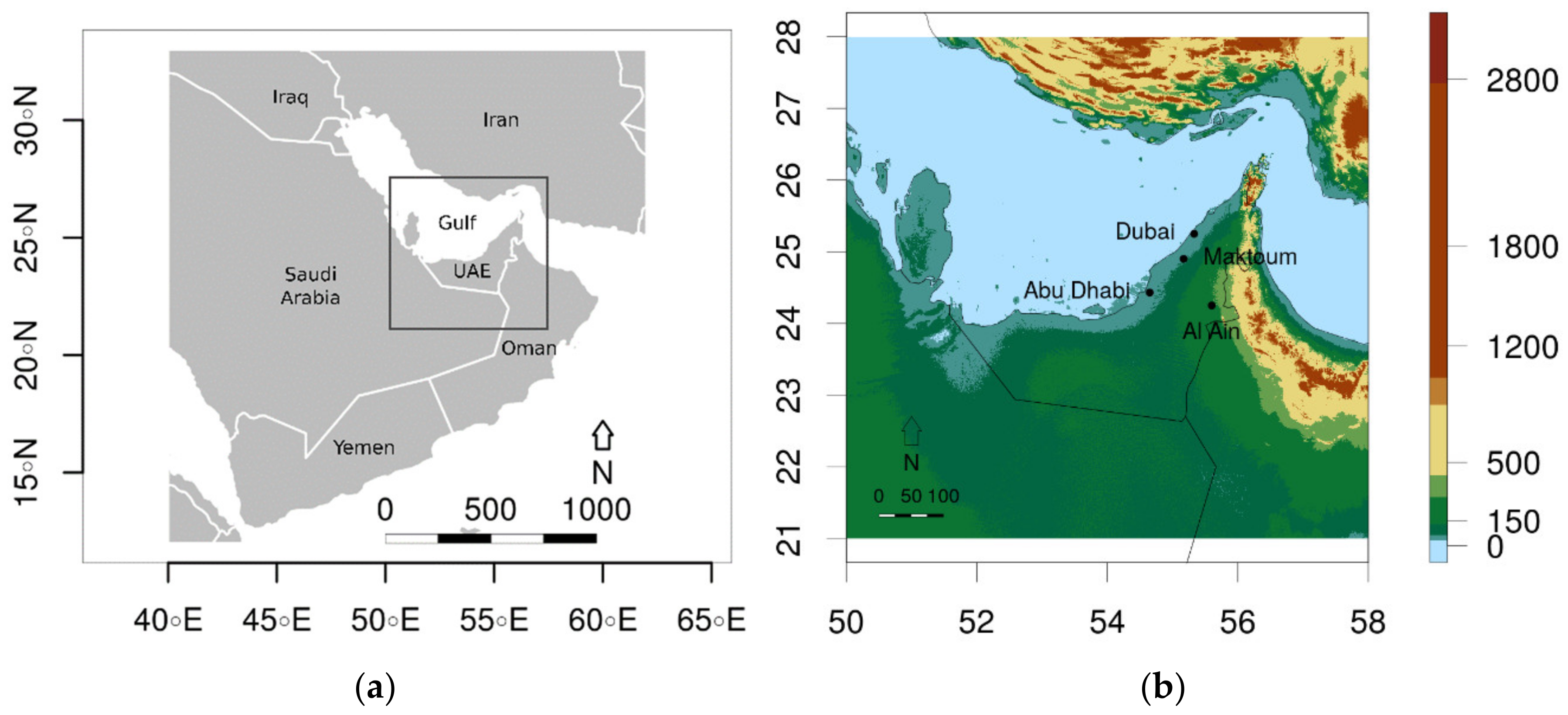
2.1. Study Area

The United Arab Emirates (UAE) is an arid country located on the northeastern edge of the Arabian Peninsula (Figure 1). It has sparse to bare vegetation and the main soil type is sand and loamy sand. It has a mean spatial annual rainfall of about 78 mm/year [13], and the dominant land cover type is bare or sparsely vegetated desert. The UAE experiences radiation fog, most frequently in winter months [14,15]. Low visibility events are more often associated with humid atmospheric conditions than with dry and dusty conditions [16,17]. The Persian Gulf is a warm and shallow water body and is located to the north of the UAE which is a source of water vapor in the atmosphere [18,19]. Fog formation requires that moisture be advected over the land from the Gulf during the day [20,21]. During the night, the land cools down quickly due to the high albedo of the desert and radiative cooling [20]. Fog forms mostly at night with peak fog occurring around sunrise [14]. Fog quickly dissipates after sunrise, although thick fog can persist until 10:00 h local time. Fog is often associated with a strong surface inversion layer [22,23]. Fog occurs most frequently over the land with a clear boundary at the coastline. The air over the Gulf is warmer at night and dew point temperature is seldom reached. Although marine fog does occur, it is less frequent than fog over the land.

2.2. Datasets

2.2.1. SEVIRI Data

SEVIRI data from Meteosat-10 situated over 9.5 °E was utilized for this study. Channel data from channel 4 (IR 3.9 µm) and 9 (IR 10.8 µm) were used in the fog detection algorithm [11,12]. The scene was subset to the region of interest and the resolution is around 3 km. Although SEVIRI data are available every 15 minutes, only hourly data (top of the hour) were used in the verification process, as they are coincident with meteorological aerodrome report (METAR) observations. The final fog mask field was further clipped to the borders of the UAE.

2.2.2. METAR Data

Meteorological aerodrome reports (METAR) were downloaded from NOAA National Climatic Data Center (NCDC) database in the integrated surface data (ISD) format. Data from four stations were used for verification, namely Abu Dhabi (OMAA, 54.65 E, 24.43 N), Dubai (OMDB, 55.33 E, 25.25 N) Al Ain (OMAL, 55.60 E, 24.25 N), and Al Maktoum (OMDW, 55.17 E, 24.90 N). These four stations have the highest frequency of fog events in the UAE [16]. Hourly and special reports (sub hourly) were used to identify fog events based on the weather description codes that indicate fog and where visibility was below 1000 m.

2.2.3. ERA5 Data

Land surface temperature from ERA5 data was used in the process of low cloud removal. ERA5 is a global atmospheric reanalysis product which is available from 1979 until the present [24,25]. Data is available hourly and at a resolution of 30 km. The data is the result of an ensemble of models, combined with observations. The land surface temperature field was downloaded from the Copernicus Climate Data Store for the months of interest [24].

2.3. Fog/Low Clouds Detection

We test a threshold-based method for detecting fog/low cloud from SEVIRI data. The method uses pseudo-emissivity (ems(3.9)), as described by Calvert and Pavolonis [11,12], to detect fog and low cloud. It uses adaptive threshold values that are determined on a pixel basis and vary monthly. The threshold was determined dynamically by modifying the method described by Cermak and Bendix [6]. In this method, the frequency distribution of pseudo-emissivity is calculated on a pixel basis. A threshold value along the distribution indicates a change in frequency, which represents a change in sky conditions. The assumption is that this threshold separates clear sky from fog cases. The threshold-based method in [6] was applied to the entire scene without accounting for potential spatial and temporal variabilities of the determined thresholds. In the present study, the threshold-based method is applied on a pixel basis while accounting for the monthly variability.
Our hypothesis is that the distribution should change in space, and thus a single threshold value across space will result in biases. A histogram of ems(3.9) was calculated per month for each pixel using a bin size of 0.032 and ranging from 0.4 to 1.072.
Pseudo-emissivity was calculated using equation (1) [11].
e m s 3.9 = R O b s 3.9 B 3.9 , B T 10.8 ,
where RObs is the radiance at 3.9 µm observed in the satellite data, BT is the brightness temperature at 10.8 µm, and B is the Planck function defined in equation (2) [26].
B v , t = C 1 v 3 e C 2 / v 1 ,
where B(ν,t) is the blackbody radiance (mW/m2-sr-cm−1), C1 = 1.19104 × 10⁻⁵ (mW/m2-sr-cm−4), C2 = 1.43877 × 10 (K cm), ν = wavenumber (cm−1), λ = wavelength (µm), and t = blackbody temperature (K).
Nighttime hours from 20:00 to 06:00 h local time were included in the sample size. The threshold value was determined from the first two values after the maximum count in the histogram, depending on which had the largest decrease in counts compared to the adjacent bin. In other words, if;
(count(indexmax)-(count(indexmax-1)) > (count(indexmax-1)-count(indexmax-2));
then
ems[index(countmax)-1] (line 1 in Figure 2);
else
ems[index(countmax)-2] (line 2 in Figure 2).
A further condition was activated if ems[index(countmax)-2] was selected, where half the bin size, 0.016 was added to the pseudo-emissivity value. A schematic of this approach is presented in Figure 2. This approach is dynamic and returns varying threshold spatially, which should result in increased verification scores.
The determination of the threshold described above is conducted by running an optimization process on the satellite data over the selected test sites. In this process, a range of threshold values for our verification sites is applied to obtain the first guess of the thresholds that should provide the best POD and FAR (described in Section 2.5) when compared to observed fog cases. Furthermore, the sensitivity of the obtained thresholds to the bin size was accounted for. Calvert and Pavolonis [11] proposed a bin size of 0.02. In this study, we found that the larger bin size of 0.032 along with the method for finding the threshold performed best for our region.

2.4. Low Cloud Detection

In the final analysis, fog and low cloud were distinguished from each other using a temperature difference method. This method makes use of an observed or proxy surface temperature value and the brightness temperature of the 10.8 channel. Similar approaches have been described by Ellrod [27] and Calvert and Pavolonis [11]. The theory here is that the window channel (10.8) is an approximation of land surface temperature for non-cloudy scenes, and cloud top temperature for cloudy scenes. When scenes are cloud free the temperature should be close to each other and when scenes contain cloud they should be further apart. ERA5 data was used in place of land surface temperature (LST) observations and 10.8 µm as the satellite brightness temperature (BT). Low cloud was defined when BT (10.8)-ERA5(LST) < −4 K. The threshold values were compared to fog cases and found to be suitable for our region. This threshold should be region-specific. An overview of the methodology is provided in Figure 3.

2.5. Verification

An assessment period of ten months, from December 2016 to March 2017 and October 2017 to March 2018, was used to determine the thresholds using a combination of collocated satellite and METAR records. This period is representative of two fog seasons. The satellite product was assessed over a 6-hour window from 00:00 to 06:00 h local time over the 10 month period. A hit is recorded when fog occurs in the METAR in any of the six hours and in the airport pixel from SEVIRI for any of the six hours (Table 1). This window was chosen as it was the period that fog was most active and it avoided sunlight hour events (solar zenith angle was greater than 90 at all verification points). Hourly matches were avoided as there was frequent contamination from higher thin cloud which affected the overall statistics. The aim was to assess daily fog frequency and not to assess hourly performance.
The probability of detection (POD), which is sometimes called hit rate, was calculated as follows:
P O D = T o t a l   h i t s T o t a l   h i t s + t o t a l   m i s s e s ,
where 1 is a perfect score. A score of 0.8 can be interpreted as 8 out of 10 observations are correctly identified. The false alarm ratio was calculated as follows:
F A R = T o t a l   f a l s e   a l a r m s T o t a l   h i t s + t o t a l   f a l s e   a l a r m s ,
where 0 is a perfect score as it would indicate no false alarms and the theoretical maximum is 1 (all events were false alarms). A score of 0.4 can be interpreted as 4 out of 10 identified events were false alarms.

3. Results and Discussion
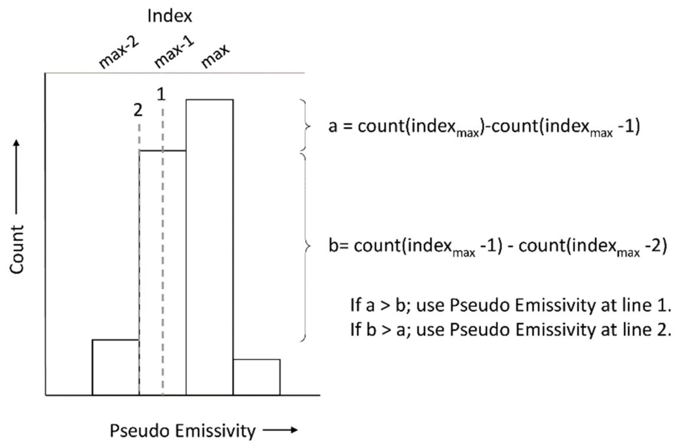
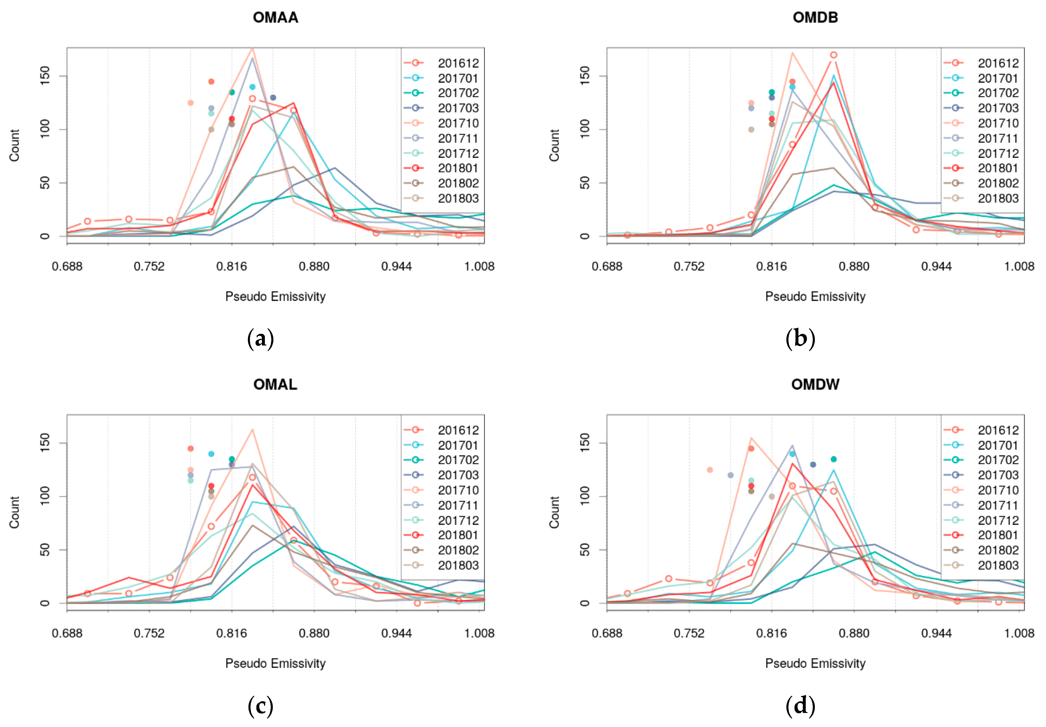
3.1. Histograms

A comparison between the optimal threshold and the calculated threshold at Abu Dhabi for January 2018 is shown in Figure 4. The optimal threshold was calculated as 0.80 (POD = 1, FAR = 0.2), while the calculated threshold was 0.82 (POD = 1, FAR = 0.33). Other months and sites (not shown) provided similar results. The similarity between the optimal and calculated thresholds demonstrate that the method used to determine the threshold value is suitable.
Initially our threshold value was indexmax-1. After the optimization, the thresholds were revised to allow lower values in some cases, which led to the inclusion of indexmax-2 (i.e., line 1 and 2 in Figure 2).
The ems(3.9) histogram shows a large spread in threshold values, which is due to the monthly variability of the calculated ems(3.9) values (Figure 5). Calvert and Pavolonis [11] found the optimal threshold to be 0.7. However, our results range from 0.78 to 0.85.
The threshold used by Calvert and Pavolonis [11] is intended for the ABI instrument on GOES-R. This instrument has a narrower bandwidth for the 3.9 µm channel of 0.2 µm compared to the SEVIRI instrument which has a bandwidth of 0.88 µm for the 3.9 µm channel [28]. SEVIRI also has a broader bandwidth for the 10.8 µm channel. This will result in different pseudo-emissivity values and alone may be the reason for the difference in threshold values.
However, three additional possibilities for this discrepancy are proposed. The first is that we use a dynamic threshold, both spatially and temporally. Our thresholds vary between sites and across the desert, which may suggest that a static threshold value may not be appropriate for the study case.
The second is a simple trade off. If we went with a more conservative threshold of 0.7, we would miss some events and decrease the POD score. In our approach we have tried to capture all possible events that were not affected by cloud cover. As such, the determined thresholds are more inclusive and may produce more false alarms. However, the third reason is that the study region is mostly homogenous in comparison to the study area in [11].
The study region in this paper is homogenous in many ways; the land cover is mostly desert, the terrain where fog forms is mostly flat/not complex, and the cloud phase is mostly warm and occurs in one season—winter. In comparison [11], study sites cover much more diverse characteristics over a larger area. As such our thresholds may be optimal for our region. Cermak [8] reported similarly in their study, that thresholds determined for Namibia may not be transferable to other regions. However, here we would like to highlight that our method in determining the threshold value is adaptive and has the potential to be transferred to other regions.

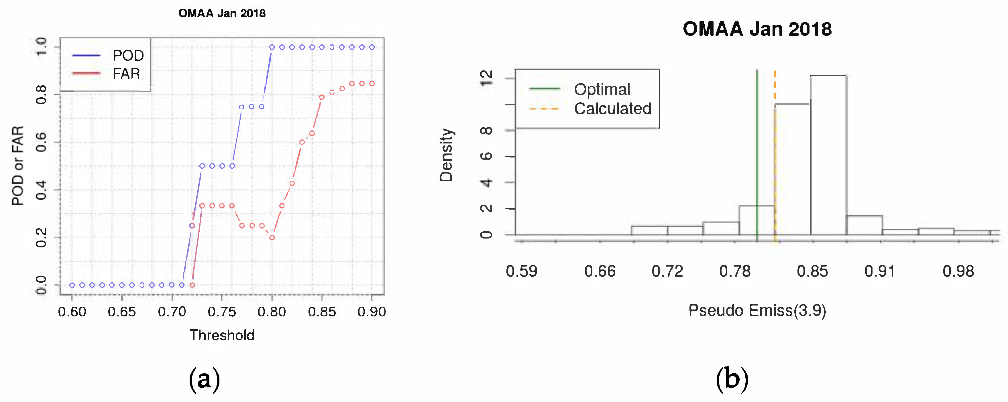
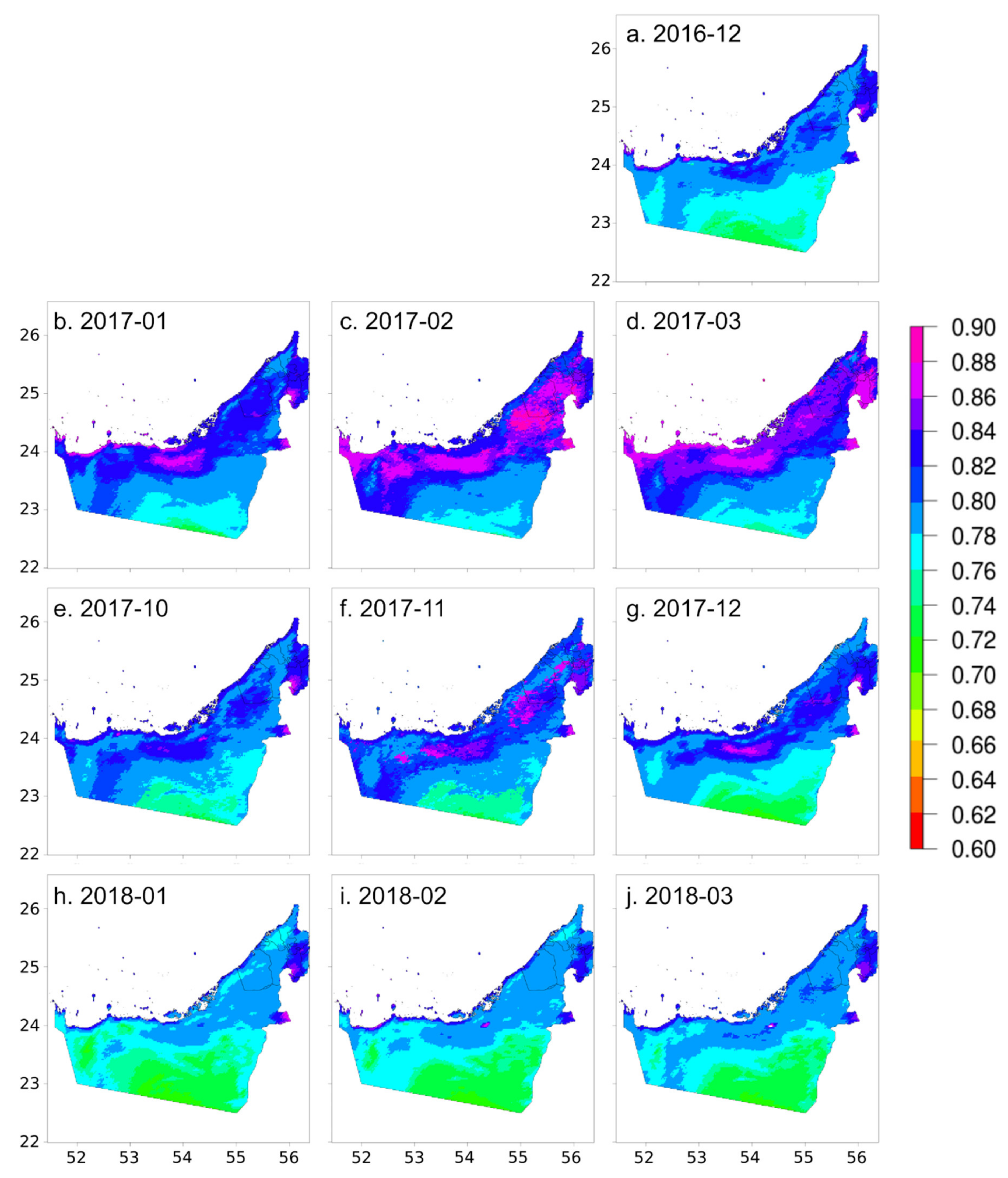
3.2. Monthly Threshold Maps: ems(3.9)

Monthly threshold maps produce similar spatial patterns of threshold values, with higher thresholds along the coast and lower thresholds further south at the start of the Empty Quarter (area of Saudi Arabia directly South of the UAE) (Figure 6). This suggests that the method accounts for the underlying spatial variation of emissivity from the desert [29], and that a spatially dynamic threshold is required for fog detection. The method shows gradual changes in spatial distribution from month to month, supporting that monthly threshold values should be used when identifying fog and low cloud. The ems(3.9) threshold shows a smooth transition from one threshold to the next along a gradient (i.e., there is no obvious inter pixel noise). This could be due to the choice of bin size in the histogram and the optimization approaches mentioned in the methodology section.
An example of the ems(3.9)-low cloud classification is shown in Figure 7 for an event at 03:00 h local time on 15 January 2018. This case is compared to the false color composite of the night microphysical product from EUMETSAT [30]. In this product, red is the difference between 12.0 and 10.8 µm channels (linear stretch −4 to 2 K), green is the difference between 10.8 and 3.9 µm channels (linear stretch 0 to 10 K) and blue is the 10.8 µm channel (linear stretch 243 to 293 K). This event is interesting as the fog patch extends across the threshold gradient from north to south, and yet is captured by the classification. This is true for many more cases (see Figures S1–S6 in the supplementary material) which corroborate that the reliability of the threshold value method is correct and should not create any spatial bias in determining fog frequency.

3.3. Assessment Over Two Fog Seasons

Here, we present the statistical verification of the ems(3.9) method over two fog seasons where 32 fog days were observed at Abu Dhabi, 12 at Dubai, 24 at Al Ain, and 30 at Al Maktoum. The first season is December 2016 to March 2017 and the second is October 2017 to March 2018, comprising 303 days in total.
The POD (FAR) was 0.81 (0.40), 0.83 (0.50), 0.83 (0.33), and 0.77 (0.44) at Abu Dhabi, Dubai, Al Ain, and Al Maktoum, respectively (Table 2). In all cases the total false alarms exceeded the total missed events, which means there is a positive bias in the fog classification. These biases were 34%, 66%, 25%, and 36% for Abu Dhabi, Dubai, Al Ain, and Al Maktoum, respectively. Of the six missed events at Abu Dhabi, three were affected by overhead cloud, two were events that occurred at 06:00 h local time (detection has a negative bias at 06:00 h), and one was due to the thick fog being thrown out as low cloud. Of the 10 missed events at Dubai, at least two were actual fog events (27 December 2016 and 25 December 2017), but surprisingly the visibility reported in the METAR was greater than 1 km. An inspection of the hourly fog masks revealed that many of the false alarms occurred when Dubai airport was on the edge of the fog event. The detection in these cases was larger than the actual event, which may be due to haze and mist at the edge of the fog being included in the classification. Thus, we suspect that the classification is including haze and mist in some cases. Similar cases of fog edge were identified for false alarms at Al Ain, although the performance at Al Ain was the best of the verification sites.
We acknowledge that further analysis, such as edge detection, can be applied to filter the false alarms and, therefore, improve the statistics which could be addressed in a future work. Other studies of nighttime fog detection have achieved lower FAR values after applying additional filters following the initial fog detection process [5,9,11,27]. Over Europe, Cermak, and Bendix [5] achieved POD (FAR) of 0.47 (0.17) using the BTD method on Meteosat SEVIRI. The low POD (below 0.5) is assigned to uncertainty in the observations by the authors. However, an important aspect in their study is that they account for the broader bandwidth of the 3.9 µm channel in SEVIRI which overlaps with CO2 absorption. This is possibly more important for scenes over Europe which have a lower viewing angle, but we note that we have not applied any such correction for our scene, which covers a much smaller area (i.e., CO2 absorption is more consistent across the scene). Application of the BTD method over desert regions and using GOES-R ABI produced POD (FAR) of 0.73 (0.14) [27]. Calvert and Pavolonis [11] applied the pseudo-emissivity method over the eastern United States (i.e., not desert) and reported POD (FAR) of 0.70 (0.15). The results from the last two studies suggest that the narrower bands on the GOES-R may allow for more distinct clustering of the histogram. Andersen and Cermak [9] applied a diurnal algorithm using SEVIRI over the Namib Desert and achieved POD (FAR) of 0.94 (0.12). In this case fog and low stratus were included in the verification, as that region experiences a high percentage of both cloud conditions. We have not included low cloud in our verification as the focus was on fog events mostly which were verified using METAR surface visibility observations. These comparisons confirm that the proposed methodology, despite its simplicity, produce a POD that is in the order of those obtained previous studies and serve as a good basis for further processing to reduce the FAR.

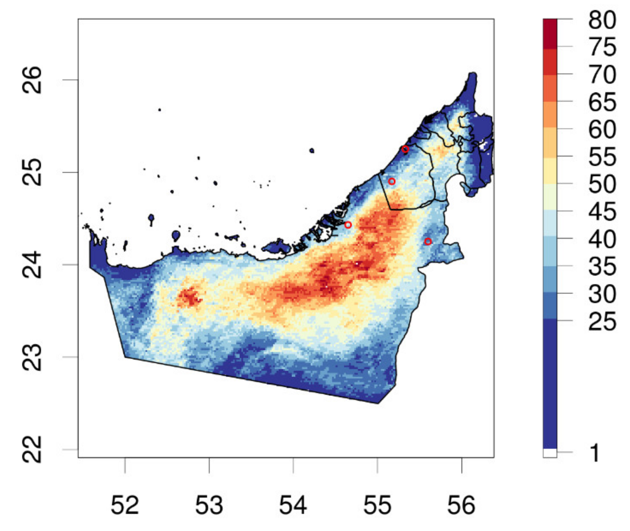
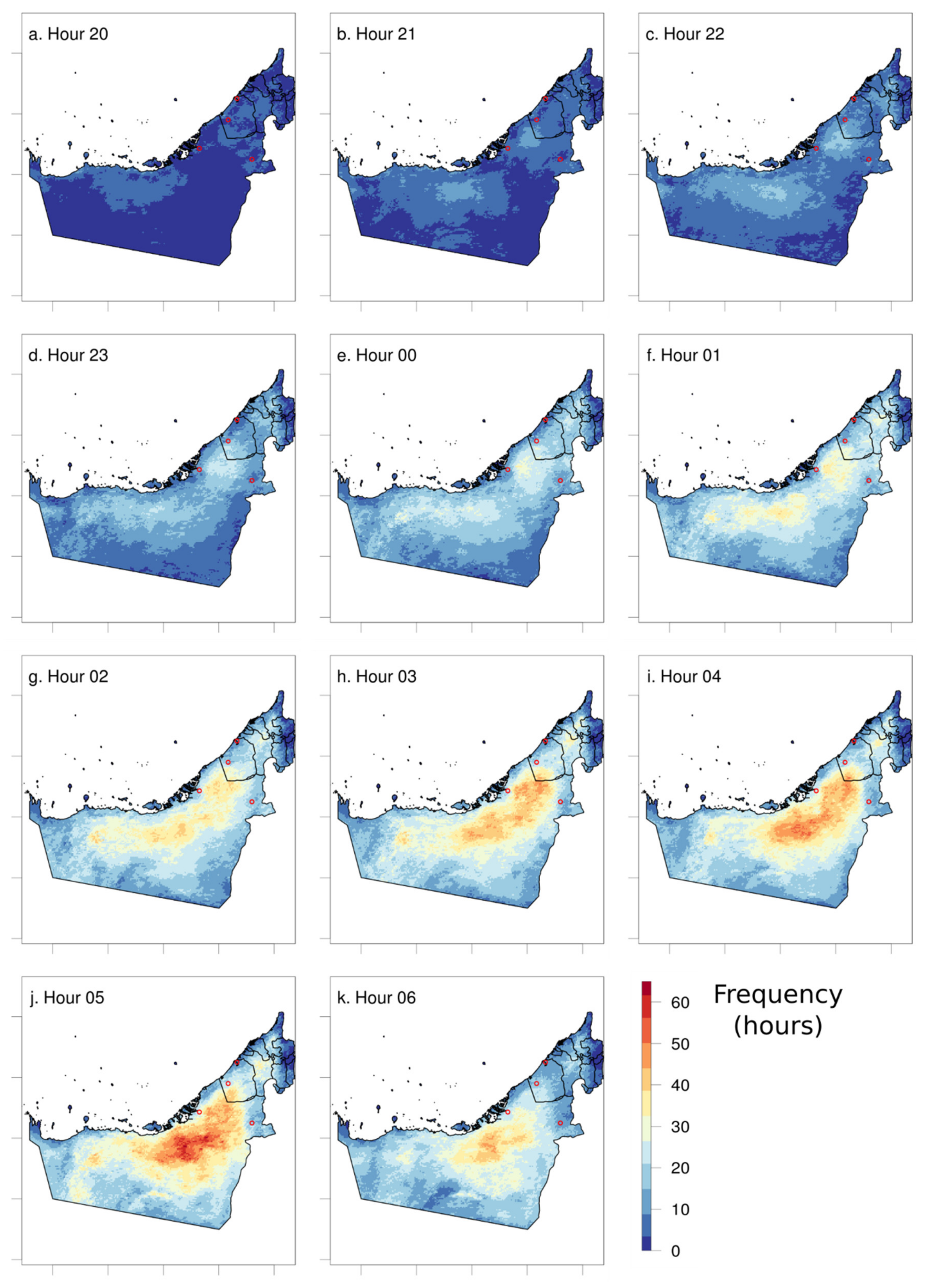
3.4. Analysis of Fog Frequency

The highest fog frequency of 80 days occurs inland and parallel to the coast, before decreasing to 25 days further inland (Figure 8). This is due to the fog dynamics in the region, which requires moisture transport from the gulf during the day and radiative cooling over the desert at night. The strip of land along the coast does not cool down as quickly as the inland desert as it is moderated by the maritime air. Thus, although it may have higher moisture content, dew point temperature is not reached as often. The area of highest fog activity is where both criteria are met: moisture is available and the air cools to dew point temperature. While further inland, fog is limited by moisture content. An interesting result is the area east of Dubai, where a small fog patch is often observed in the hourly maps that is disconnected from larger fog patches. This area is a strip of narrow land between the coast and the Hajar Mountains and most likely has slightly different dynamics in fog formation than the larger, inland fog patch.
The spatial distribution of fog days indicates that our verification sites occur outside the area of maximum fog activity. This supports the earlier statement that the stations are often at the edge of fog patches. The maximum value reported is 80 days of fog out of a maximum of 303 days in the sample. This may be an overestimate of 25% to 35 %, in line with the Abu Dhabi and Al Ain results presented in Table 2. However, this should not affect the spatial distribution, which would remain similar even if the magnitude was adjusted (i.e., scaled down). Upon inspection of hourly fog masks, we found the classification to be in line with the distributions seen here. To our knowledge, this is the first time the spatial distribution of fog over the UAE has been presented and verified.
Information on fog, the timing of fog formation, and its distribution throughout the UAE could be inferred from Figure 9. Two areas are visible as hot spots for fog formation, which are clearly demonstrated in the 21:00 h (local time) panel in Figure 9. The first area is situated between the three verification stations of Abu Dhabi, Dubai, and Al Ain (over the Sweihan desert) and the other is South West of Abu Dhabi. These areas remain visible up until hour 02:00 h when they merge. Thus, fog onset is much earlier in these hotspot areas.
The hourly maps do reveal a diurnal cycle that is in line with previously published results from the METAR observations [14]. Fog frequency increases as night progresses, highlighting the dependence on radiative cooling for fog formation. This is consistent with the obtained results especially those related to the spatial pattern of fog frequency, which may suggest that the proposed algorithm for determining the threshold does not require additional adjustment to account for diurnal variability, which seems to be correctly captured in Figure 9. Fog is shown to peak at 05:00 h local time and then decrease at 06:00 h. This is not in line with METAR observations which show that fog frequency is highest at 06:00 h and 07:00 h [14]. Thus, we should expect 06:00 h to be higher, however, analysis revealed a systematic bias at 06:00 h. Although we included 06:00 h in the sample as the solar zenith angle was greater than 90 (below the horizon), it is possible that there is some reflection at the top of the atmosphere, which increase the ems(3.9) value to increase above the threshold value. This is only expected to occur in October and March.

4. Discussion

The following limitations have been identified in this study and are recommended for further refinement in future studies. The negative bias at 06:00 h can most likely be corrected for by removing the reflected component of the radiance in the satellite observations. This should be useful as 06:00 h is still a nighttime hour and it will improve the verification and the diurnal cycle maps.
The method for removing low cloud could be improved upon. While it appears to work for our case, we identified potential issues, most notably that there is a diurnal cycle of the difference between BT(10.8) and LST(ERA5). This makes sense for cloud cases, where there is a lag between surface cooling and upper air cooling. As such, the constant threshold of −4 K used in this study may need to be adjusted diurnally. In some cases, low cloud was classified when no cloud was present. This can be for various reasons, like upper air dust or thin cloud [31], or a bias in the ERA5 data. However, these cases did not coincide with fog detection, and did not degrade the performance of the fog classification.
Haze and mist were often included in the classification, either in the hours preceding fog onset or at the edge of fog patches. These could potentially be reduced through a layer thickness approach similar to Cermak (2012) [8], where they calculate cloud top height to determine cloud thickness. The assumption here is that haze and mist may return lower cloud top heights than fully developed fog, but this remains to be tested.

5. Conclusions

In this paper we present the assessment of the pseudo-emissivity method for nighttime fog detection using the SEVIRI instrument from Meteosat-10. The method is similar to the one proposed for the GOES-R ABI which is largely untested with SEVIRI data. In addition, we implement an adaptive threshold method that allows the threshold to vary spatially and temporally. The spatial variation reduces the number of false alarms in the fog classification. The study area was the United Arab Emirates (UAE), a desert region on the Arabian Peninsula that experiences extensive fog during the winter months. The method verified well, with POD (FAR) ranging from 0.77 to 0.83 (0.33 to 0.5). We present the fog frequency for 10 months when fog is present over the UAE. This is the first time the spatial distribution of fog has been presented seamlessly across the UAE using satellite data. Previous studies relying on scarce station data did not capture the full spatial pattern of fog formation in the country and its dynamics. The fog classification had a positive bias, ranging from 25% to 66 %, mostly due to the inclusion of haze and mist in the classification. The hourly frequency is presented and is in line with in situ measurements, indicating peak fog frequency at 05:00 h local time. The results confirm that the pseudo-emissivity method is a reliable separator for fog detection in the UAE using SEVIRI data.

Supplementary Materials

The following are available online at https://www.mdpi.com/2072-4292/12/14/2281/s1, Figure S1. Examples of hits at Abu Dhabi at 2016-12-07 0200 (a–d) and Al Ain at (c,d). Times in UTC. Figure S2. Example of cloud effected fog days. The cloud in the RGB has a ems(3.9) above the threshold value and is not captured in the fog mask. Times in UTC. Figure S3. Example of miss at Al Ain. Although this was a miss at one location, the patch was still well represented and will, correctly, form part of the fog frequency map. Times in UTC. Figure S4. Example of false alarms at Dubai (a,b) and Abu Dhabi (c,d). Although images a-b are false alarms in the METAR, a fog patch is visible in the RGB adjacent to the airport. The patch is well represented and considered correct in terms of the fog frequency. The image c,d has no fog in the RGB and is a total false alarm. Times in UTC. Figure S5. Example of a false classification outside of airports. Although no fog was classified at any of the airports, there is a general over estimate of fog in this scene in the interior. This may contribute to an overestimation of fog frequency. Times in UTC. Figure S6. Examples of underestimation of fog at 06:00 h local time (UTC+4). This is most likely due to reflection at the top of the atmosphere just before sunrise. Times in UTC.

Author Contributions

Conceptualization, methodology, validation, formal analysis, writing—original draft preparation, M.W.; conceptualization, methodology, writing—review and editing, supervision, M.T. All authors have read and agreed to the published version of the manuscript.

Funding

Funding from Etihad Airways to support the research with focus on fog formation in the UAE.

Acknowledgments

The authors acknowledge the assistance of Mohan Thota for converting data formats of the satellite data.

Conflicts of Interest

The authors declare no conflict of interest.

References

  1. Gultepe, I.; Sharman, R.; Williams, P.D.; Zhou, B.; Ellrod, G.; Minnis, P.; Trier, S.; Griffin, S.; Yum, S.S.; Gharabaghi, B.; et al. A Review of High Impact Weather for Aviation Meteorology. Pure Appl. Geophys. 2019, 176, 1869–1921. [Google Scholar] [CrossRef]
  2. Yousef, L.A.; Temimi, M.; Wehbe, Y.A. Total cloud cover climatology over the United Arab Emirates. Atmos. Sci. Lett. 2019, 20, 1–10. [Google Scholar] [CrossRef]
  3. Eyre, J.R.; Brownscombe, J.L.; Allam, R.J. Detection of fog at night using Advanced Very High Resolution Radiometer (AVHRR) imagery. Meteorol. Mag. 1984, 113, 266–271. [Google Scholar]
  4. Turner, J.; Allam, R.J.; Maine, D.R. A case-study of the detection of fog at night using channels 3 and 4 on the Advanced Very High-Resolution Radiometer (AVHRR). Meteorol. Mag. 1986, 115, 285–290. [Google Scholar]
  5. Cermak, J.; Bendix, J. Dynamical nighttime fog/low stratus detection based on Meteosat SEVIRI data: A feasibility study. Pure Appl. Geophys. 2007, 164, 1179–1192. [Google Scholar] [CrossRef]
  6. Cermak, J.; Bendix, J. A novel approach to fog/low stratus detection using Meteosat 8 data. Atmos. Res. 2008, 87, 279–292. [Google Scholar] [CrossRef]
  7. Nilo, S.T.; Romano, F.; Cermak, J.; Cimini, D.; Ricciardelli, E.; Cersosimo, A. Fog detection based on Meteosat Second Generation-Spinning enhanced visible and infrared imager high resolution visible channel. Remote Sens. 2018, 10, 541. [Google Scholar] [CrossRef] [Green Version]
  8. Cermak, J. Low clouds and fog along the South-Western African coast—Satellite-based retrieval and spatial patterns. Atmos. Res. 2012, 116, 15–21. [Google Scholar] [CrossRef]
  9. Andersen, H.; Cermak, J. First fully diurnal fog and low cloud satellite detection reveals life cycle in the Namib. Atmos. Meas. Tech. 2018, 11, 5461–5470. [Google Scholar] [CrossRef] [Green Version]
  10. Egli, S.; Thies, B.; Bendix, J. A hybrid approach for fog retrieval based on a combination of satellite and ground truth data. Remote Sens. 2018, 10, 628. [Google Scholar] [CrossRef] [Green Version]
  11. Calvert, C.; Pavolonis, M. GOES-R Advanced Baseline Imager (ABI) Algorithm Theoretical Basis Document for Low Cloud and Fog; University of Wisconsin-Madison Space Science and Engineering Center: Madison, WI, USA, 2010. [Google Scholar]
  12. Pavolonis, M.J.; Heidinger, A.K. Advancements in identifying cirrus and multilayered cloud systems from operational satellite imagers at night. Appl. Weather Satell. II 2005, 5658, 225. [Google Scholar] [CrossRef]
  13. Ouarda, T.B.M.J.; Charron, C.A. Evolution of the rainfall regime in the united arab emirates. J. Hydrol. 2014, 514, 258–270. [Google Scholar] [CrossRef] [Green Version]
  14. De Villiers, M.; Van Heerden, J. Fog at Abu Dhabi international airport. Weather 2007, 62, 209–214. [Google Scholar] [CrossRef] [Green Version]
  15. TS, M.; Temimi, M.; Ajayamohan, R.S.; Fonseca, R.; Weston, M.; Valappil, V. On the investigation of the typology of fog events in an arid environment and the link with climate patterns. Mon. Weather Rev. 2020. [Google Scholar] [CrossRef]
  16. Aldababseh, A.; Temimi, M. Analysis of the long-term variability of poor visibility events in the UAE and the link with climate dynamics. Atmosphere 2017, 8, 242. [Google Scholar] [CrossRef] [Green Version]
  17. Karagulian, F.; Temimi, M.; Ghebreyesus, D.; Weston, M.; Kondapalli, N.K.; Valappil, V.K.; Aldababesh, A.; Lyapustin, A.; Chaouch, N.; Hammadi, F.A.; et al. Analysis of a severe dust storm and its impact on air quality conditions using WRF-Chem modeling, satellite imagery, and ground observations. Air Qual. Atmos. Health 2019, 1–18. [Google Scholar] [CrossRef] [Green Version]
  18. Elhakeem, A.; Elshorbagy, W.; Bleninger, T. Long-term hydrodynamic modeling of the Arabian Gulf. Mar. Pollut. Bull. 2015, 94, 19–36. [Google Scholar] [CrossRef]
  19. Sheppard, C.; Al-Husiani, M.; Al-Jamali, F.; Al-Yamani, F.; Baldwin, R.; Bishop, J.; Benzoni, F.; Dutrieux, E.; Dulvy, N.K.; Durvasula, S.R.V.; et al. The Gulf: A young sea in decline. Mar. Pollut. Bull. 2010, 60, 13–38. [Google Scholar] [CrossRef]
  20. Bartok, J.; Bott, A.; Gera, M. Fog Prediction for Road Traffic Safety in a Coastal Desert Region: Improvement of Nowcasting Skills by the Machine-Learning Approach. Bound.-Layer Meteorol. 2012, 157, 501–516. [Google Scholar] [CrossRef]
  21. Weston, M.; Chaouch, N.; Valappil, V.; Temimi, M.; Ek, M.; Zheng, W. Assessment of the Sensitivity to the Thermal Roughness Length in Noah and Noah-MP Land Surface Model Using WRF in an Arid Region. Pure Appl. Geophys. 2018. [Google Scholar] [CrossRef]
  22. Temimi, M.; Fonseca, R.M.; Nelli, N.R.; Valappil, V.K.; Weston, M.J.; Thota, M.S.; Wehbe, Y.; Yousef, L. On the analysis of ground-based microwave radiometer data during fog conditions. Atmos. Res. 2020, 231, 104652. [Google Scholar] [CrossRef]
  23. Chaouch, N.; Temimi, M.; Weston, M.; Ghedira, H. Sensitivity of the meteorological model WRF-ARW to planetary boundary layer schemes during fog conditions in a coastal arid region. Atmos. Res. 2016, 187, 106–127. [Google Scholar] [CrossRef]
  24. Copernicus Climate Change Service (C3S). ERA5: Fifth Generation of ECMWF Atmospheric Reanalyses of the Global Climate, Copernicus Climate Change Service Climate Data Store (CDS). 2017. Available online: https://climate.copernicus.eu/climate-data-store (accessed on 4 May 2018).
  25. Hersbach, H.; Bell, B.; Berrisford, P.; Hornyi, A.; Sabater, J.M.; Nicolas, J.; Radu, R.; Schepers, D.; Simmons, A.; Soci, C.; et al. Global reanalysis: Goodbye ERA-Interim, hello ERA5. ECMWF Newsl. 2019, 17–24. [Google Scholar] [CrossRef]
  26. Cao, C.; Shao, X. Planck Function. Available online: https://ncc.nesdis.noaa.gov/data/planck.html (accessed on 26 September 2019).
  27. Ellrod, G.P. Estimation of low cloud base heights at night from satellite infrared and surface temperature data. Natl. Weather Dig. 2002, 26, 39–44. [Google Scholar]
  28. Dammann, K.; Mueller, J.; Hanson, C.; Gartner, V.; Flewin, J.; Williams, M. MSG level 1.5 image data format description. EumetsatDarmstadtTech 2005, 3, 1–129. [Google Scholar]
  29. Hulley, G.C.; Hook, S.J.; Abbott, E.; Malakar, N.; Islam, T.; Abrams, M. The ASTER Global Emissivity Dataset (ASTER GED): Mapping Earth’s emissivity at 100 meter spatial scale. Geophys. Res. Lett. 2015, 42, 7966–7976. [Google Scholar] [CrossRef]
  30. EUMETSAT. Best Practices for RGB Compositing of Multi-Spectral Imagery; User Service Division, EUMETSAT: Darmstadt, Germany, 2009; p. 8. [Google Scholar]
  31. Weston, M.J.; Temimi, M.; Nelli, N.R.; Fonseca, R.M. On the Analysis of the Low-Level Double Temperature Inversion Over the United Arab Emirates : A Case Study During April 2019. IEEE Geosci. Remote Sens. Lett. 2020. [Google Scholar] [CrossRef]
Figure 1. (a) The United Arab Emirates (UAE) is located on the Arabian Peninsula. (b) Terrain (m.a.s.l.) and location of meteorological aerodrome report (METAR) stations used for verification.
Remotesensing 12 02281 g001
Figure 2. Schematic indicating how the threshold value was selected based on the histogram of pseudo-emissivity at each pixel.
Remotesensing 12 02281 g002
Figure 3. Overview of the Spinning-Enhanced Visible and Infrared Imager (SEVIRI) fog detection methodology. Gray boxes represent data layers and white boxes represent data processing. The numbers on the arrows represent the path on the first and second iteration, respectively. This method was applied per pixel and over a one-month period for each month in the study period.
Remotesensing 12 02281 g003
Figure 4. (a) Example of calculated optimal threshold at Abu Dhabi (OMAA) for January 2018. Here the optimal threshold is 0.80 (POD = 1, FAR = 0.2). (b) The calculated threshold was 0.82.
Remotesensing 12 02281 g004
Figure 5. Histogram of ems(3.9) at (a) Abu Dhabi (OMAA) (b) Dubai (OMDB), (c) Al Ain (OMAL) and (d) Al Maktoum (OMDW). Monthly threshold values are indicated by closed circles on the pseudo-emissivity plots. Placement on the y-axis is arbitrary for these dots in order to avoid concealment from overlap.
Remotesensing 12 02281 g005
Figure 6. Spatial distribution of monthly threshold value of ems(3.9) from (ad) December 2016 to March 2017 and (ej) October 2017 to March 2018.
Remotesensing 12 02281 g006
Figure 7. (a) Example of ems(3.9)-low cloud fog classification in comparison with (b) the EUMETSAT night microphysical product [30] for 2018-01-15 0300 local time.
Remotesensing 12 02281 g007
Figure 8. Fog frequency in days for ems(3.9)—low cloud over the 10 month period. Verification sites are indicated by red circles.
Remotesensing 12 02281 g008
Figure 9. Hourly fog frequency from 20:00 h to 06:00 h local time.
Remotesensing 12 02281 g009
Table 1. Contingency table.
METAR Fog YesMETAR Fog No
SEVIRI fog yesHitsFalse Alarms
SEVIRI fog noMissesCorrect Negative
Table 2. Dec 2016–Mar 2018.
OMAAOMDBOMALOMDW
Statisticems(3.9)—Low Cloudems(3.9)—Low Cloudems(3.9)—Low Cloudems(3.9)—Low Cloud
Total Hits26102023
Total Miss6247
Total False Alarms17101018
POD0.810.830.830.77
FAR0.400.500.330.44
Bias score1.341.661.251.36

