A Comparative Study of Estimating Auroral Electron Energy from Ground-Based Hyperspectral Imagery and DMSP-SSJ5 Particle Data

Abstract

Aurora, the spectacular phenomenon commonly occurring in high latitudes, is caused by the precipitation of energetic particles penetrating the Earth’s atmosphere. Being the result of solar-terrestrial interactions, electron precipitation significantly contributes to auroral production. To evaluate its magnitude, a physical quantity describing the characteristics of precipitating auroral electrons—their characteristic energy—is adopted. In this paper, this quantity is derived from joint data observed by the ground-based auroral spectroscopic imager located in Antarctica Zhongshan Station and the particle detectors “Special Sensor J5 (SSJ5)” on the Defense Meteorological Satellite Program (DMSP) satellites. A postprocessing scheme of ground-based spectral data is proposed to infer the characteristic energy that successively uses classical brute-force, recursive brute-force and self-consistent approximation strategies for step-up speed improvement. Then, the inferred characteristic energies are compared to the average energies calibrated from the relevant electron data detected by SSJ5 to confirm whether this inference is valid. Regarding DMSP F18/SSJ5, these two energy estimations about auroral electrons deviate slightly from each other and show a strong linear relationship. It sheds light on further applications of the valuable aurora spectral data.

1. Introduction

Solar activities interact with Earth’s atmospheric environment in multiple ways so that cause various natural phenomenon, change the climate, and affect electronic communications in our daily life. The interactions between the sun and Earth are driven by energetic particles, a portion of which enter the Earth near its magnetic poles, precipitate in the atmosphere, and cause ionization, optical emissions, etc. The atmospheric optical emissions are referred to as aurorae. Studies on them provide a way to understand how the atmosphere responds to the penetration of auroral particles [1,2,3] and unveil the very nature of solar-terrestrial interactions [4,5,6].

As the name suggests, auroral particles are the particles that induce aurora, most of which are electrons. Being an indirect indicator of the intensity of atmospheric precipitation and solar-terrestrial activities, the electron characteristic energy is investigated by drawing the help from both in situ and ground-based detections. In the former case, satellites [7,8,9] and sounding balloons [10] facilitate the direct electron measurements, in which the Special Sensor J5 (SSJ5) particle detector on the Defense Meteorological Satellite Program (DMSP) satellite monitors the electrons and protons along its orbital track with a 90° field of view (FOV). By contrast, ground-based instruments like all-sky imagers (ASI) [11,12], auroral spectrograph (ASG), etc. prevail for long-term observations. The first attempt to infer the characteristics energy of auroral electrons from the remotely-sensed data by these instruments was [13], focusing on the emission rate of 472.8 nm and three intensity ratios 630.0/427.8, 557.7/427.8 and 630.0/557.7 for inference. This work derived from simulating the temporal characteristics of ion densities and composition concerning a typical aurora [14,15]. Recently in [16], the characteristics of precipitating electrons were estimated for an “inverted-V” aurora event from ground-based emission data of 427.8, 557.7 and 844.6 nm by using the modified GLobal airglOW (ModGLOW) model [17]. Their comparison with the detected energies by Ground-to-Rocket Electrodynamics-Electrons Correlative Experiment (GREECE) shows the feasibility of such estimations. Besides, [18] analyzed the auroral radiations over Lowell, MA on 22–23 June 2015, and derived the precipitating electron energy and flux by using the GLobal airglOW (GLOW) model [19].

The inverse problem to solve the precipitation characteristics of auroral particles from ground-based data is difficult to achieve in practice, so the above-related studies all centre on modelling the auroral production instead. Models describing electron transportation in the atmosphere are used for the simulation of auroral emissions, considering that the precipitation electrons are the main energy source of aurorae. Starting from the exploration of the relationship between the relative atomic oxygen abundance and emissions of 427.8, 486.1, 630.0, 732.0 and 844.6 nm in the thermosphere [20], the Electron TRANSport (ETRANS) model was developed on the basis of an electron transport equation derived by applying altitude and energy boundary conditions to the Boltzmann equation [21]. Boltzmann 3-Constituent (B3C) [22] simulates the auroral electron precipitation by solving a Fokker–Planck equation, while Atmospheric Ultraviolet Radiance Integrated Code (AURIC) [23] takes the calculated data by B3C to model the airglow emissions in the far-ultraviolet and near-infrared. The application of [24] to electron transport equations led to the tomographic inversion of 630.0 nm emission [25,26], following by the development of GLOW based on Monte Carlo techniques. GLOW was later modified in various ways: employing a hybrid Monte Carlo/Two-stream (MC2S) to auto-solve the fluxes of auroral protons, hydrogen atoms and secondary electrons [27], involving the far-ultraviolet emissions of N₂ LBH band system, 135.6 nm and 149.3 nm doublets [28], updating the radiative and chemistry parameters with the latest data [17] and so on.

Essential for understanding the solar-terrestrial system, observations that monitor the auroral phenomena have been carried out at Chinese research stations in Antarctica and Arctic. Raw data generated by ground-based instruments are generally used to create the time-versus-latitude plots called keograms [29] that represent the time-evolution of auroras. Then, researchers familiar with relevant studies undertake a further study based on these plots. However, the truth is that these data per se contain much more auroral information to be represented. With this into consideration, this paper aims to provide an in-depth application of these data, so that even people who are new to solar-terrestrial research can have a comprehensive view of Earth’s atmospheric environment.

In this paper, the auroral electron energy is inferred from the ground-based aurora spectral data (ASD) (provided by the Meridian Space Weather Monitoring Project) generated by the ASG equipped in Chinese Zhongshan Station (located at 76.38°E, 69.37°S) (ZHS) [30,31]. To infer this energy as fast as possible, the strategies that make the simulated auroral events converge to the real events retrieved from these spectral data in brute-force, recursively brute-force and self-consistent manners are developed. The estimation of auroral electron energy from the data observed by ASG is compared to the estimation from DMSP F16–F18 satellite data jointly observed with ASG for a mutual validation between both estimations.

The rest of this paper is structured as follows. Section 2 describes ASG and ASD in details essential for the following sections. Section 3 proposes our adopted model for simulating the electron transportation and three different approximation strategies used for estimating the auroral electron energy from ASD based on this model. Section 4 presents the respective implementations of these strategies concerning a specific frame of ASD. Section 5 introduces the procedures of estimating the auroral electron energy from the observed electron data by SSJ5, then compares the estimated energies from both ASD and F16~F18 SSJ5 data. Section 6 summaries the paper.

2. Ground-Based Hyperspectral Imagery

At ZHS, auroral characteristics are currently acquired with the help of an enhanced synchronous observation system [32]. Besides ASG, this system consists of multiwavelength all-sky imagers, multiscale imagers and a radiometer. Up to now, many auroral studies have been presented on the basis of their observed data [33,34,35].

ASG, the instrument exclusively used for the spectroscopic observations of aurorae occurring over ZHS, acquires auroral spectral information along the magnetic meridian and could produce successive frames of ASD every 20 s. As illustrated in Figure 1, it comprises of six units: (1) a fish-eye lens with 180° FOV, (2) a slit with the width of 0.07 mm that controls the light flux, (3) a relay lens, (4) a grism dispersing the incident light into several monochromatic components, (5) a fixed focus lens, and (6) an electron-multiplying charge-coupled device (EMCCD) Andor DU8201 which is the key assembly for photoelectric conversion.

Each frame of ASD is generated within 15 s and formatted as Flexible Image Transport System (FITS) file. Containing not only hyperspectral information but also morphological information about aurorae, such a file stores a fixed number of 16-bit digital counts that can be visualized as an image with a size of 1024 × 1024. Figure 2 illustrates an example ASD frame. The horizontal and vertical axes represent the magnetic latitude and bandwidth linearly varying with the position index, respectively, and the spectral and spatial resolutions are determined by spectrograph calibrations. Analogous to the pixel value as to images, each digital count can be accessed by using its corresponding spatial and spectral position indexes together.

3. The Scheme to Estimate the Precipitating Electron Energy

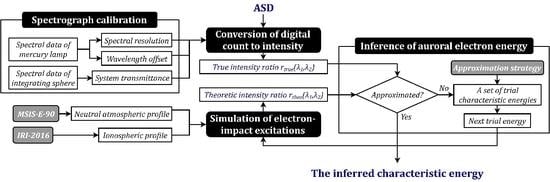
3.1. Schematic Diagram and Some Basic Concepts

The major procedures of deriving the auroral electron characteristic energy from raw ASD are indicated by the black rounded rectangles in Figure 3. They center on the conversion of true intensity ratio from digital counts after calibrating the spectrograph ASG, and successive computation of the theoretical ratio by substituting different trial characteristic energies into an electron transport model until both ratios are approximate enough. Besides, the adopted approximation strategy determines the set of trial characteristic energies, so affects the overall time spent for the derivation.

It is apparent that the intensity ratios between two optical emissions are the key intermediate for derivation. The true ratio relates to the constitution of the spectroscopic system. As mentioned in the previous section, the imaging unit of ASG is an Andor EMCCD camera with the sensor CCD201-20. Using the knowledge about EMCCD imaging and count conversion concerning Andor cameras [36], the true ratio concerning the emissions of ${\lambda }_1$ and ${\lambda }_2$ can be expressed as follows if ASG is regarded as an equivalent EMCCD sensor.

$$r_{\mathrm{true}}\left({\lambda }_1,{\lambda }_2\right)=\frac{p_{{\lambda }_1}}{p_{{\lambda }_2}}\cdot \frac{Q{E}_{{\lambda }_2}{T}_{{\lambda }_2}^{*}}{Q{E}_{{\lambda }_1}{T}_{{\lambda }_1}^{*}}$$

(1)

In Equation (1), $p_{\lambda }$ is the spectrally-averaged digital count with respect to the emission of $\lambda$, while $QE$ and $T^{*}$ denote the sensor’s quantum efficiency value and the equivalent system transmittance, respectively. The digital counts of each emission are averaged in the spectral dimension because it covers several spectral position indexes in practice due to line broadening effect [37].

On the other hand, the intensity ratio can be numerically calculated as $r_{\mathrm{theo}}$ in Equation (2) by using an electron transport model which requires inputting the energy spectrum of auroral electrons. For modelling, the absolute emission intensity is expressed in the unit of column emission rate $\epsilon$. Due to the difficulty in quantitatively measuring the column length for a light beam, it is the integral of volume emission rate $\eta$ over the available range of altitude $h$.

$$\begin{gathered} r_{\mathrm{theo}}\left({\lambda }_1,{\lambda }_2\right)=\frac{\epsilon \left({\lambda }_1\right)}{\epsilon \left({\lambda }_2\right)} \\ \epsilon \left(\lambda \right)={{\displaystyle \int }}_0^{\infty }\eta \left(\lambda ,h\right)dh \end{gathered}$$

(2)

According to the basic principles of spectroscopy, optical emission accompanies with energy loss when an atom or molecules undergo the transition between different energy levels. For instance, a particle $X$ loses energy by emitting a photon of the particular wavelength with a certain probability if it is excited from a low-level energy state $l_0$ to a high-level state $u$ and finally stays in a state $l$ that has the energy lower than $u$ but higher than $l_0$. In this case, the volume emission rate is related to the transition probability $A_{u\to l}$, namely Einstein A coefficient of transition $u\to l$, and the number density of the particles of the upper state $n_u$ as follows.

$$\eta \left(\lambda \right)=A_{u\to l}\cdot n_u$$

(3)

Being the important physical quantity for calculating the absolute intensity and relative intensity ratio, $n_u$ is simulated by using the electron transport model described in the next subsection.

3.2. The Modified Rees’s Electron Transport Model

Here the electron-impact excitation part of [15], which models the major reaction to excite the atmospheric neutral constituents, is modified to simulate the transportation of precipitating electrons. Given the electron energy spectrum, this modified model requires the profiles of neutral atmosphere and initial ionosphere as the input, implements the equations from (4) to (10), and finally returns the time derivative of $n_u$. Among these equations, (7)–(9) are referred from the papers of [14], [38] and [39], respectively.

Table 1. Units for physical quantities.

Symbol	Quantity	Common Unit a	Equation Number
ε	Column emission rate	R	(2)
η	Volume emission rate/Production rate	cm−3 s−1	(2)–(7)
A	Transition probability	s−1	(3), (4)
a	Deactivation coefficient	cm3 s−1	(4)
n	Number density	cm−3	(3)–(5), (8), (10)
Φ	Flux	cm−2 s−1 eV−1	(5), (6)
E	Energy	eV/keV	(5)–(10)
σ	Cross section	cm2	(5), (10)
f	Shape factor	eV−1	(7)
ρ	Mass density	g cm−3	(8)
z	Atmospheric depth	g cm−2	(8)
dE/dx	Stopping power	eV cm−1	(9), (10)

^a R = Rayleigh [40], cm = center miter, s = second, eV = electron volt, keV = kilo electron volt, g = gram.

gives the units of physical quantities.

$$\partial n_u/\partial t={\eta }_u-[A_u+{\displaystyle \sum }_i^{N}a\left(Q_i\right)n\left(Q_i\right)]n_u$$

(4)

$${\eta }_u=n_0{{\displaystyle \int }}_{E_{th}}^{\infty }{\Phi }_s\left(E_s,h\right){\sigma }_{0u}\left(E_s\right)d{E}_s$$

(5)

$${\Phi }_s\left(E_s\right)={{\displaystyle \int }}_{E_s}^{\infty }\frac{{\eta }_s\left(E\right)dE}{\left(\frac{dE}{dx}{|}_{\mathrm{ele}}+\frac{dE}{dx}{|}_{\mathrm{neut}}\right)}$$

(6)

$${\eta }_s\left(E_s\right)=\frac{{{\displaystyle \sum }}_{i=1}^3{S}_{X_i}{f}_{X_i}\left(E_s\right)}{{{\displaystyle \sum }}_{i=1}^5{S}_{X_i}{f}_{X_i}\left(E_s\right)}\cdot q$$

(7)

$$\begin{array}{c}q=n_0{\displaystyle {\int }_{E_{p\min }}^{E_{p\max }}\frac{{\rho }_{z_{\max }}}{z_{\max }\Delta E_{\mathrm{ion}}}}\cdot \frac{n{(M)}_z}{n{(M)}_{z_{\max }}}\cdot \Lambda (z/z_{\max })\cdot n(E_p)E_{p}d{E}_p\\ z(h)={\displaystyle {\int }_h^{\infty }\rho }(h^{\prime })d{h}^{\prime }\begin{array}{cc},& z_{\max }=4.57\times {10}^{-6}{E}_p^{1.75}\end{array}\end{array}$$

(8)

$$\frac{dE}{dx}{|}_{ele}=\{\begin{array}{c}\frac{{\omega }_p^2{e}^2}{\nu }ln\frac{m{\nu }^3}{\gamma e^2{\omega }_p},kT\le E_s\le \frac{m{e}^4}{2{\hslash }^2}\\ \frac{{\omega }_p^2{e}^2}{\nu }ln\frac{m{\nu }^2}{\hslash {\omega }_p},E_s>\frac{m{e}^4}{2{\hslash }^2}\end{array}$$

(9)

$$\frac{dE}{dx}{|}_{neut}={\displaystyle \sum }_{i}n\left(X_i\right){\displaystyle \sum }_j{W}_{ij}{\sigma }_{ij}\left(E_s\right)$$

(10)

The overall production of excited particles is primarily contributed by electron-impact excitation and reduced by the quenching effect. Variables $A_u$, $n$ and $a$ in Equation (4) represent the spontaneous emission rate of the excited particles, the number density and the collisional deactivation coefficient concerning the quenching species $Q_i$, respectively. Equation (5) calculates for the volume emission rate of these particles. Regarding this equation, $n_0$ is the number density of particles in the initial state $l_0$, $E_{th}$ the threshold energy in the unit of eV, ${\mathsf{\Phi }}_s$ the altitude-dependent differential secondary electron flux and ${\sigma }_{0u}$ the energy-dependent excitation cross section.

For secondary electrons, Equations (6) and (7) are combined to solve their flux $\mathsf{\Phi }$ and production rate ${\eta }_s$. $E_s$ is their energy in the unit of eV, ${\left(dE/dx\right)|}_{\mathrm{ele}}$ is the stopping power of these electrons, while ${\left(dE/dx\right)|}_{\mathrm{neut}}$ is that of the neutral gas. Denoted by $X_1$~$X_5$, N₂, O₂, N, He and H are five major neutral constituents in the atmosphere. Their weights $S_{X_1}$~$S_{X_5}$ are 1.15, 1.5, 0.56, 0.43 and 0.8, respectively. $f$, the shape factor that determines the energy distribution of secondary electrons, depends on the energies of both primary (auroral) and secondary electrons.

Directly determining the production rate of secondary electrons, the total ionization rate $q$ weakly depends on the energy distribution of primary electrons. As given in Equation (8), it is obtained by integrating the modulated differential energy flux of primary electrons $n\left(E_p\right)E_{p}d{E}_p$ over $\left(E_{p\min },E_{p\max }\right)$, where the unit of $E_p$ is keV and the upper limit of the primary energy interval is normally taken as a value much larger than the lower limit. In this integral function, $\mathsf{\Delta }{E}_{\mathrm{ion}}$ is the energy loss to produce an ion pair and $\mathsf{\Lambda }$ is the energy dissipation function. $n{\left(M\right)}_z$ is the total number densities at the atmospheric depth $z$ calculated by purely using the mass density profile, while $n{\left(M\right)}_{z_{\max }}$ corresponds to the maximum atmospheric depth $z_{\max }$ that is directly decided by the primary electron energy.

Equations (9) and (10) both express the stopping powers. When to calculate the stopping power of secondary electrons, there are two cases distinguished by the magnitude of their energy. In their corresponding equations, $m$, $e$, $\nu$ and $T$ are the mass, charge, speed and temperature of electrons, respectively, and ${\omega }_p$ is the frequency of electron plasma, $ln\gamma$ is the Euler’s constant equal to 0.577. With respect to the neutral stopping power, $W_{ij}$ denotes the excitation potential and ${\sigma }_{ij}$ the excitation cross section for a transition from level $X_i$ to $X_j$.

In fact, Equation (4) is a first-order linear differential function because the production rate ${\eta }_u$ is indeed independent of time. Thus, it can be theoretically and experimentally inferred that $n_u$ converges to a limit value within a certain time, as expressed by Equation (11). This coincides with common sense that the excited particle loses energy in its lifetime until becoming stable.

$$n_u\left(t\right)=\frac{{\eta }_u}{A_{u\to l}+{{\displaystyle \sum }}_i^{N}a\left(Q_i\right)n\left(Q_i\right)}$$

(11)

Then, the absolute intensity of emission $\lambda$ is derived by combining Equations (2), (3) and (11).

$$\epsilon \left(\lambda \right)={{\displaystyle \int }}_0^{\infty }{A}_{u\to l}{\eta }_{\lambda ,u}/[A_u+{\displaystyle \sum }_i^{N}a\left(Q_{\lambda ,i}\right)n\left(Q_{\lambda ,i}\right)]dh$$

(12)

Accordingly, the theoretical intensity ratio is

$$r_{\mathrm{theo}}\left({\lambda }_1,{\lambda }_2\right)=\frac{{{\displaystyle \int }}_0^{\infty }{A}_{u_1\to l_1}{\eta }_{{\lambda }_1,u}/\left[A_{u_1}+{{\displaystyle \sum }}_i^{N}a\left(Q_{{\lambda }_1,i}\right)n\left(Q_{{\lambda }_1,i}\right)\right]dh}{{{\displaystyle \int }}_0^{\infty }{A}_{u_2\to l_2}{\eta }_{{\lambda }_2,u}/\left[A_{u_2}+{{\displaystyle \sum }}_i^{N}a\left(Q_{{\lambda }_2,i}\right)n\left(Q_{{\lambda }_2,i}\right)\right]dh}$$

(13)

3.3. Approximation Strategies

3.3.1. Classical Brute-Force Approximation

In most cases, the energy spectrum of precipitating electrons follows either a Maxwellian or an exponential distribution [38,41,42], that is, $n\left(E_p\right)E_{p}d{E}_p=n_{\alpha }{e}^{-E_p/\alpha }d{E}_p$ or $n\left(E_p\right)E_{p}d{E}_p=n_{\beta }{e}^{-\beta }d{E}_p$. $\alpha$ and $\beta$, the parameters determine the distribution shape, are in the unit of keV. Accordingly, the energy-independent number fluxes $n_{\alpha }$ and $n_{\beta }$ are in the unit of cm⁻² s⁻¹ keV⁻¹. Defined as the ratio of energy flux to number flux [43] given in Equation (14), the characteristic energy of auroral electrons is $\alpha$ or $\beta /2$ if these electrons are Maxwellian- or exponential-distributed. These characteristic energies are just the auroral characteristics to be derived in this paper.

$$\langle E_p\rangle =\frac{{\displaystyle \int }{n}_p{E}_{p}d{E}_p}{{\displaystyle \int }{n}_{p}d{E}_p}$$

(14)

As described above, the absolute intensity of any emission can be simulated from such an energy spectrum with the help of electron transport model, but it is difficult to reverse this simulation because the simulated intensity is an integration over the altitude range. Taking this into consideration, the strategies concerning approximation solving are considered for calculating the characteristics of electrons from the intensities of certain emissions induced by these electrons.

Let $P_N$ be the profile of the neutral atmosphere, $P_I$ the initial ionospheric profile and $E$ the trial value of the characteristic energy ($\alpha$ or $\beta /2$), the function representing the electron transport model is denoted by $r_{\mathrm{theo}}=DeduceRatio\left(P_N,P_I,E\right)$. The preliminary simulations show that $r_{\mathrm{theo}}$ increases with the trial energy $E$. On this basis, the core of approximation solving is to take successively the value of $E$ from a set of energies until the intensity ratio $r_{\mathrm{theo}}$ simulated by using this model is approximate to the true ratio $r_{\mathrm{true}}$ converted from the digital counts of ASD. Then, the auroral characteristic energy is estimated as the last trial energy.

Using the brute-force approximation strategy, it is simple to estimate the auroral characteristic energy by increasing $E$ with a step of $dE$ from the initial energy $E_l$ and terminating this increment once $r_{\mathrm{theo}}\approx r_{\mathrm{true}}$. In this paper, the termination condition holds when the absolute difference between both ratios is no more than $5\times {10}^{-5}$.

3.3.2. Recursive Brute-Force Approximation

To improve the computational efficiency of brute-force solving, fast implementation is developed by dynamically adjusting the energy increment $dE$. Algorithm 1 provides its pseudo code, the major part of which is a nested while loop that controls the iterative increment of $E$, of which the outer and inner loops adjust the incremental step $dE$ and the incremental interval $\left(E_l,E_r\right)$, respectively. Besides, $r_r$ denotes the calculated ratio in the current iteration, while $r_l$ stores the ratio of the last iteration. According to the monotonic direct relationship between the calculated ratio and trial energy, it can be derived that the characteristic energy is within $\left(E_l,E_r\right)$ if $r_{\mathrm{true}}$ falls into the interval $\left(r_l,r_r\right)$. In such cases, the inner loop is terminated early with the adjusted $\left(E_l,E_r\right)$ being the incremental interval of E for the following iterations, meanwhile, the incremental step is reduced by a factor of 10. The iteration number largely decreases due to the autoscaling of iterative steps, while the precision concerning the estimation of characteristic energy remains the same as the traditional brute-force strategy.

Algorithm 1. The brute-force strategy

Input: The true intensity ratio $r_{\mathrm{true}}$ Output: The trial characteristic energy $E$ Initialize: $E_l=-0.9$, $E_r=10.1$, $dE=0$, $r_l=0$, $r_r=0$ Algorithm:  while $E_l<E_r$ do   $E\leftarrow E_l+dE$ $E=E_l+dE$   while $E<E_r$ do    $r_r=DeduceRatio\left(P_N,P_I,E\right)$    if $\left|r_r-r_{\mathrm{true}}\right|<5\times {10}^{-5}$ then     $E_l=E_r$     break    end if    if $r_{\mathrm{true}}>r_l$ and $r_{\mathrm{true}}<r_r$ then     $E_r=E$     break    end if    $E_l=E$    $r_l=r_r$    $E=E+dE$   end while    $dE=dE/10$  end while

3.3.3. Recursive Brute-Force Approximation

The computational complexities of the described brute-force strategies are somewhat high for practical applications. Thus, the self-consistent approximation strategy as represented in Algorithm 2 is developed for a further speedup. This strategy implements the self-consistent convergence of $E$ by using only one while loop that adaptively updates $k$.

The experimentally observed quasilinear relationship between the simulated intensity ratio and trial value of characteristic energy, which is manifested as $r=E·k$, ensures the self-consistency of approximation solving. It also accords with the empirical conclusion drawn by analyzing the dayside arc data jointly acquired from DMSP and instruments in the Chinese Arctic Yellow River Station [44].

Algorithm 2. The recursive strategy.

Input: The true intensity ratio $r_{\mathrm{true}}$ Output: The trial characteristic energy $E$ Initialize: $k=k_0$, $r_{\mathrm{theo}}=0$ Algorithm:  while $\left|r_r-r_{\mathrm{true}}\right|\ge 5\times {10}^{-5}$ do   $E=r_{\mathrm{true}}/k$   $r_{\mathrm{theo}}=DeduceRatio\left(P_N,P_I,E\right)$   $k=r_{\mathrm{theo}}/E$  end while

4. An Example—Derivation

Among all the visible emissions contained by ASD, the ones with wavelengths of 557.7 and 630.0 nm appear yellow-green and red, respectively. They both are the optical signatures of Earth’s auroras caused by the excitation of oxygen atoms, so here we focus on them for the following derivation. Essential for the ratio calculation concerning their true intensities based on Equation (1), $QE$ and $T^{*}$ are 94.2% and 91.0% regarding emission 557.7 nm, and are 92.7% and 63.4% regarding emission 630.0 nm, respectively. For any emission, the calculated true ratios are dependent on the spatial position index indicating the viewing zenith angle of ASG.

Regarding Figure 2, $r_{\mathrm{true}}$ equals to 6.3966 taken as the maximum ratio in terms of all spatial positions. It is used by different approximation strategies for deriving the characteristic energy of auroral electrons. Then, the auroral productions for different characteristic energies are simulated under the assumption that the simulated auroral electrons are typical, viz. Maxwellian-distributed. This is accomplished by using the electron transport model DeduceRatio to calculate a number of theoretical ratios between the intensities of emissions 557.7 and 630.0 nm. Certain atmospheric parameters are required by this model, including number densities of N₂, O₂, N, He and H, total mass density, electron density, and temperatures of neutral constitutes, electrons and ions within the altitude range of 80~1000 km above ZHS. These parameters are calculated with the help of Mass Spectrometer Incoherent Scatter Extension 1990 (MSIS-E-90) [45] and International Reference Ionosphere 2016 (IRI-2016 [46] that model the neutral atmosphere and ionosphere, respectively.

Table 2. Parameters used in the electron transport model.

λ (nm)	557.7	630.0
u→l	O(1S)→O(1D)	O(1D)→O(3P)
Eth (eV)	4.18	1.96
Au→l (s−1)	1.26	6.478 × 10−3 a
Au(s−1)	1.26	8.58 × 10−3 a
Q1~QN	O2, O	N2, O2
a(Q1)~a(QN) (s−1)	1 × 10−13, 2 × 10−13	8 × 10−11, 3 × 10−11

^a Referred from [48].

lists other essential parameters for $DeduceRatio$, where the transition probabilities and deactivation coefficients except the ones with superscripts are referred from [47].

When the recursive brute-force approximation is adopted, the trial value of characteristic energy $E$ is initialized to increment by 1 keV every iteration from 0.1 keV.

Table 3. Iterative variation of the incremental step dE and incremental interval (E_l, E_r) of trial energy in the recursive brute-force derivation regarding Figure 2.

Incremental Step dE (eV)	Trial Energy E (eV) (Theoretical Ratio rr)	Updated Interval (El,Er)
1000	1010 (3.1)→2010 (6.1)l→3010 (9.2)r→	(2010,3010)
100	2110 (6.44)r→	(2010,2110)
10	2020 (6.16)→2030 (6.19)→2040 (6.22)→2050 (6.25)→2060 (6.28)→ 2070 (6.31)→2080 (6.34)→2090 (6.38)l→2100 (6.41)r→	(2090,2100)
1	2091 (6.378)→2092 (6.381)→2093 (6.384)→2094 (6.387)→2095 (6.391)→ 2096 (6.394)l→2097 (6.3967)r→	(2096,2097)
0.1	2096.1 (6.3939)→2096.2 (6.3942)→2096.3 (6.3945)→2096.4 (6.3948)→ 2096.5 (6.3951)→2096.6 (6.3954)→2096.7 (6.3957)→2096.8 (6.3961)→ 2096.9 (6.3964)l→	(2096.9,2097)
0.01	2096.91 (6.3964)→2096.92 (6.3964)→2096.93 (6.3964)→2096.94 (6.3965)→2096.95 (6.3965)→2096.96 (6.39654)→2096.97 (6.39657)

represents the specific derivation process of Figure 2. In this table, the number in the bracket denotes the theoretical ratio calculated by inputting the trial energy listed before this bracket into $DeduceRatio$. Superscripts “l” and “r” mark the energy-ratio pairs corresponding to the updated lower and upper bounds of the incremental interval $\left(E_l,E_r\right)$, respectively. It can be observed that the incremental step $dE$ has auto-scaled for five times until becoming 0.01 eV, and at last the characteristic energy corresponding to the true ratio of 6.3966 is estimated to be 2096.97 eV. To sum up, there are 37 iterations executed in total. By contrast, if using the classical brute-force strategy with $dE$ set as 0.01 eV to guarantee that the estimation error is still less than $5\times {10}^{-5}$, the electron transport model should run 199,697 times. Undoubtedly, the recursive brute-force strategy is much more efficient.

On this basis, the energy-ratio pairs corresponding to the iterations given in Table 3 are plotted as points in the “${\log }_{10}(E)$-${\log }_{10}(r_r)$” coordinate system, as represented in Figure 4. Equation (15) expresses the line fitted by using these points, in which case both the Pearson correlation and adjusted R-Square coefficients are more than 99.9%. The slop of the fitted line is pretty close to 1, suggesting a linear relationship between the trial characteristic energy $E$ and theoretical ratio $r_r$ which is just the basic of performing the self-consistent approximation.

$${log}_{10}(r_r)=1.0093{log}_{10}(E)+0.4813$$

(15)

As to this approximation, Figure 5 represents its implementations for different initial values of $k$. For each implementation, the characteristic energy is estimated as 2096.98 eV. From this figure, it can be seen that the trial energy $E$ approximates to this estimation after only one iteration and converges within few iterations. Though the initialization of $k$ does not affect the estimated results, it influences the time overhead of self-consistent approximation. The processing time reduces when $k$’s initial value is close to its true value. For instance, this true value is 100.4813 ≈ 3.029 according to Equation (15) and there are fewest iterations performed when $k=3$. In addition, the self-consistent strategy exhibits a significant improvement in convergence speed than the brute-force ones as it decreases the number of iterations by about ten times, from 37 to three or four, so it is adopted for the practical derivations with $k$ always initialized as three for simplicity.

5. Experimental Studies

Limited by the current techniques, any in situ instrument cannot provide the continuous energy spectra of its measured particles. Under this circumstance, because there are no standard data served as a basis for comparison, the estimation about auroral electron energy by using the above-described scheme cannot be validated unless other estimations being considered for comparative validation. In this section, two estimations based on the ASD and SSJ5 data acquired during the joint observations of ASG and DMSP satellites, respectively, are compared for validating each other. Clearly, if one of them agrees with the other, our proposed scheme is feasible.

5.1. Joint Observations by ASG and DMSP SSJ5

DMSP satellites are in their respective polar-orbits that pass above or nearly above Earth’s poles with an orbital period of about 101 min. Each of them sometimes observes the same regions of the atmosphere as ASG. As particles within the loss cone will precipitate in the atmosphere, a portion of the energetic particles characterized by SSJ5 cause the auroral emissions imaged by ASG. Thus, SSJ5 and ASG could form a joint observing system.

Observations by SSJ5 and ASG are considered as joint when satisfying: the geographic distance between a DMSP satellite and ZHS is small, which means this satellite passes over ZHS and is likely to capture the precipitating auroral electrons. Such distances are calculated by using the respective two-line element sets for F16~F18 satellites, and here the ASD and SSJ5 data corresponding to distances of no more than 50 km are selected for performing the comparative estimations.

Besides, ASG scans along the magnetic meridian with a finite FOV and DMSP satellite passes the plane of this meridian through a specific position. As represented in Figure 6, the effective FOV is indicated by the green curve while the trajectory of the satellite is in blue. The intersection of the green and blue curves is just the cross point through which this satellite passes the magnetic meridian plane, corresponding to the viewing zenith angle of ${\alpha }_1$. Assuming that ASG has a maximum viewing zenith angle of ${\alpha }_{\max }$, there is no doubt that the data generated when ${\alpha }_1$ is more than ${\alpha }_{\max }$ should be removed from the already-selected joint data because the DMSP satellite is out of ASG’s FOV in such cases.

5.2. Estimation Concerning the Particle Energy Data Detected by SSJ5

Up to now, the practicability of SSJ5 has been proved by a series of successful observations and its applications. The first launched SSJ5 monitored the particles of KeV and MeV during the 2003 Halloween Storms [49]. Then, the empirical relationship between the acquired data by Special Sensor Ultraviolet Spectrographic Imager (SSUSI) and SSJ5 was investigated for their conversion [50]. It is presented in [51] that F19/SSJ5 confirmed its passage through the cusp so as to provide the basis for solving the tomographic reconstruction problem concerning the cusp.

This device divides into six sections to count the number of electrons and ions incident in its discrete energy channels of specific energies within the range of 30 eV~30 keV [52]. In the mode of data acquisition, it returns the sum of particle counts from all sections by second. These summed counts are 9-bit words consisting of 4-bit exponents and 5-bit mantissas, which are log-compressed for telemetering and then log-uncompressed in the ground stations. Air Force Research Laboratory (ARFL) developed a calibration algorithm for the uncompressed counts to attenuate the influence of penetrating particles. According to the description in [52], the mean energy of the detected particles in a specific second (denoted by ${\overline{E}}_{\mathrm{SSJ}}$) is estimated from the corresponding calibrated count by using the following equation:

$$\begin{gathered} J_i=\frac{C_i}{G_i\cdot \Delta t},J{E}_i=J_i{E}_i \\ J={\displaystyle \sum }_i{J}_i\Delta E_i,JE={\displaystyle \sum }_{i}J{E}_i\Delta E_i \\ {\overline{E}}_{\mathrm{SSJ}}=\frac{JE}{J} \end{gathered}$$

(16)

where $\Delta t$ is the channel integration time, $C_i$, $E_i$, $\mathsf{\Delta }{E}_i$, $G_i$, $J_i$, $J{E}_i$ are the calibrated count, mean energy, differential energy, channel geometric factor, calibrated particle flux and calibrated particle energy flux corresponding to the $i$-th energy channel, respectively. These parameters are provided in [53].

In the combination of Equations (14) and (16), the definitions of $\langle E_p\rangle$ and ${\overline{E}}_{\mathrm{SSJ}}$ are similar. Recall that each frame of ASD is generated within 15 s, so $\langle E_p\rangle$ indicates the averaged characteristic energy over the exposure time. Accordingly, the 1-s mean energies ${\overline{E}}_{\mathrm{SSJ}}$ of captured particles throughout the joint observation by SSJ5 are averaged and the averaged ${\overline{E}}_{\mathrm{SSJ}}$ is denoted by $\langle E_{\mathrm{SSJ}}\rangle$ to be consistent with $\langle E_p\rangle$.

Generally lasting for 10~20 s, the duration of joint observation is adjusted to further ensure the consistency of the estimated ASD and SSJ5 data. Taking an example, if a joint observation event starts at $t_0$ and ends at $t_1$, while ASG starts to expose at $t_2$ and a frame of ASD is generated 15 s later, then the starting and ending times of this event should be adjusted as $t_0=max\left(t_0,t_2\right)$ and $t_1=\min \left(t_1,t_2+15\right)$, respectively.

5.3. Comparative Estimations Based on the Joint Observations

In this subsection, our estimations of the auroral electron energy from ASD are compared to the estimations from the joint data generated by SSJ5 detectors on the on-orbit DMSP satellites, namely F16, F17 and F18. It is mentioned above that for our estimation, the true intensity ratio of a specific spatial position index is used for deriving $\langle E_p\rangle$. Here the true ratio of the spatial position index corresponding to the viewing zenith angle of ASG at the satellite is taken for the comparison because there is a linear mapping between such indexes and ASG’s viewing zenith angles.

In the visualized ASD frame of Figure 6, the region between green lines represents the acquired atmospheric information, while the red line represents the information about the cross point of the DMSP satellite that is remotely-sensed by ASG and the tag ${\alpha }_1$ below this line denotes the viewing zenith angle of ASG when DMSP passes the magnetic meridian plane. Applying the sine law to the red triangle shown in Figure 7, this angle is calculated from

$$\frac{sin{\alpha }_1}{R+h}=\frac{sin({\alpha }_1-\beta )}{R}$$

(17)

where $\beta$ is the geocentric angle, $R$ and $h$ are the radius of the earth and the altitude of the DMSP satellite, respectively.

On this basis, the joint observation events since 2013 are analyzed and the estimations about the characteristic energy of auroral electrons are compared for these events. Relevant results are given in

Table 4. Estimations from both auroral spectral data (ASD) and acquired data by Special Sensor J5 (SSJ5) particle detector concerning various joint observing events.

Satellite	Day	Frame	$\langle {\mathit{E}}_{\mathit{p}}\rangle \left(\mathbf{eV}\right)$	$\langle {\mathit{E}}_{\mathrm{SSJ}}\rangle \left(\mathbf{eV}\right)$	${\mathit{t}}_1-{\mathit{t}}_0 \left(\mathbf{s}\right)$	${\mathit{t}}_{\mathbf{eff}} \left(\mathbf{s}\right)$
F16	13/05/31	134903	262.1	285.9	8	8
	13/07/15	223614	609.1	145.9	14	7
	13/07/31	223243	527.6	8026.8	11	1
	13/08/08	223051	318.5	5806.7	14	1
	13/08/16	222858	253.2	187.2	8	6
	13/08/18	134406	234.7	1472.4	15	15
	13/09/03	134027	245.5	2698.8	14	14
	13/09/16	223435	300.8	567.3	7	5
	13/09/24	223245	237.8	141.1	11	7
	14/04/09	221632	435.0	93.6	9	4
	14/04/25	221113	354.6	220.8	14	8
	14/06/29	131721	225.1	332.6	12	12
	14/07/20	220700	309.0	97.8	5	4
F17	13/06/17	230821	303.0	189.6	7	7
	13/06/19	142314	245.4	123.8	6	6
	13/07/18	231147	235.9	189.5	5	5
	13/08/03	230707	424.5	170.0	11	11
	13/08/11	230443	258.0	175.7	8	4
	13/08/26	231257	364.9	135.9	11	10
	13/09/03	231036	341.5	180.3	10	7
	13/09/11	230800	392.0	194.1	10	10
	13/09/19	230541	355.4	117.2	10	10
	14/04/01	231257	364.9	170.8	14	10
	14/04/26	143045	535.2	123.0	13	10
	14/08/18	231620	320.9	200.5	7	7
F18	13/05/13	163600	281.6	292.9	15	13
	13/05/28	012655	251.3	316.3	10	10
	13/06/06	011810	285.5	47.2	10	6
	13/07/10	163610	269.5	181.5	10	10
	13/08/03	011818	322.6	181.1	6	6
	13/08/11	012139	239.4	175.4	12	12
	13/08/19	012501	229.5	530.5	9	9
	13/10/01	163401	335.6	388.8	6	6
	14/06/30	011110	1124.6	1060.2	5	5
	14/07/25	010740	288.4	126.7	12	12

. The column of “Frame” gives the creation times of ASD, for example, the frame “134,903” is created at 13:49:03 UT. Besides, SSJ5 produce unusable negative counts once performing the anomaly detection concerning particles, so its acquired data under such circumstances should be ignored for calculating $\langle E_{\mathrm{SSJ}}\rangle$ and the total time of effective detection for each joint observing event is listed in the column of $t_{\mathrm{eff}}$.

Clearly, the deviation between both estimations cannot be avoided since the measured particles by SSJ5 are not always the ones detected by ASG. From this table, it can be observed that the larger of the estimated auroral characteristic energies $\langle E_p\rangle$ and $\langle E_{\mathrm{SSJ}}\rangle$ is several times the smaller in most cases. However, they differ significantly from each other if the effective detection of SSJ5 lasts for a short time. For instance, when one second of SSJ5′s acquired data is used for the energy estimation, $\langle E_p\rangle$ and $\langle E_{\mathrm{SSJ}}\rangle$ are 527.6 and 8026.8 eV, respectively, or 318.5 and 5806.7 eV. Also, this significant difference happens for the case that SSJ5 carries out a long-time (14 or 15 s) effective detection.

For the events corresponding to F16~F18 satellites, the average differences between $\langle E_p\rangle$ and $\langle E_{\mathrm{SSJ}}\rangle$ are 1414.5, 180.9 and 118.8 eV, respectively, while the standard deviations are 2293.6, 93.5 and 86.9 eV. Accordingly, the corresponding ratios of the average energy difference to the average energy deviation are 395.7%, 49.5% and 42.5%. It can be concluded that the energies estimated by using the observed data from F17 and F18 satellites are more similar to our estimated energies.

Besides, $\langle E_p\rangle$ varies with the event more gently than $\langle E_{\mathrm{SSJ}}\rangle$. Its standard deviation is 161.6 eV, while that of $\langle E_{\mathrm{SSJ}}\rangle$ is 1622.1 eV. As illustrated in Figure 8, our estimated energies are within the derivation range of the estimated energies by using the data from F18 satellite. The fact is that $\langle E_p\rangle$ is relevant to $\langle E_{\mathrm{SJJ}}\rangle$ with a high correlation coefficient of 0.85 with respect to this satellite. However, the differences between $\langle E_p\rangle$ and $\langle E_{\mathrm{SSJ}}\rangle$ are mostly beyond the standard deviation range of any of them regarding the F16 satellite.

6. Conclusions

Being the manifestation of atmospheric optical emissions, aurora phenomenon is caused by the particle precipitation. In this paper, the joint observed data by ground-based hyperspectral imaging and satellite-borne particle detection are used for estimating the characteristic energy of auroral electrons. The estimation from spectral data is accomplished with the help of our proposed scheme that obtains such energies by approximating the modelled intensity ratio between emissions 557.7 and 630.0 nm to a value considered as the true ratio. The classical brute-force, recursive brute-force and self-consistent approximation strategies are successively developed for the progressive improvements in the whole computation efficiency. Further, this estimation is compared to the estimation based on the detected electron data by SSJ5 sensors on the DMSP satellites.

The auroral electron characteristic energies estimated from both ground-based ASD and DMSP SSJ5 data inevitably deviate from each other. However, their comparison reveals that there is a strong correlation between our estimation and the estimation based on F18/SSJ5 data. This reveals the possibility to jointly use remotely sensed and in situ data for investigating the auroral characteristics. Furthermore, the validity of our proposed scheme is confirmed in a somewhat indirect way.

This scheme considerably uses the implicit atmospheric information of the spectral data, which fills the vacancy in the related studies about aurora spectral data of ZHS. However, the atmospheric processes that take place are too complex to be simulated. Moreover, the ground-based hyperspectral imagery of auroral emissions inevitably differs from the in situ detection of these emissions because of their attenuation in passing through the atmosphere. For a wide application of estimating the auroral characteristics, these shortcomings should be addressed.

Fortunately, including sufficient atmospheric physical and chemical reactions in the simulation of electron transportation ensures the estimation accuracy to a certain extent, so this is one direction of our future work. Taking the attenuation effect into account also benefits the further modification of our proposed scheme and helps correct the difference between the estimations from ASD and SSJ5 data. The goal of such corrections is to make the estimation from remotely sensed imagery close to that from in situ data, but, as mentioned above, only a part of the detected particles by SSJ5 will induce the atmospheric optical emissions observed by ASG, indicating that this difference cannot be eliminated. Considering this, determining the cross-calibration factor between both ground-based and in situ data is an attractive attempt.

References

1. Ergun, R.; Andersson, L.; Main, D.; Su, Y.J.; Newman, D.; Goldman, M.; Carlson, C.; Hull, A.; McFadden, J.; Mozer, F. Auroral particle acceleration by strong double layers: The upward current region. J. Geophys. Res. Space Phys. 2004, 109, A12220. [Google Scholar] [CrossRef] [Green Version]
2. Newell, P.T.; Sotirelis, T.; Wing, S. Diffuse, monoenergetic, and broadband aurora: The global precipitation budget. J. Geophys. Res. Space Phys. 2009, 114, A09207. [Google Scholar] [CrossRef]
3. Ni, B.; Thorne, R.M.; Zhang, X.; Bortnik, J.; Pu, Z.; Xie, L.; Hu, Z.-J.; Han, D.; Shi, R.; Zhou, C. Origins of the Earth’s diffuse auroral precipitation. Space Sci. Rev. 2016, 200, 205–259. [Google Scholar] [CrossRef]
4. Sandholt, P.; Farrugia, C.; Stauning, P.; Cowley, S.; Hansen, T. Cusp/cleft auroral forms and activities in relation to ionospheric convection: Responses to specific changes in solar wind and interplanetary magnetic field conditions. J. Geophys. Res. Space Phys. 1996, 101, 5003–5020. [Google Scholar] [CrossRef]
5. Kozlovsky, A.; Safargaleev, V.; Østgaard, N.; Turunen, T.; Koustov, A.; Jussila, J.; Roldugin, A. On the motion of dayside auroras caused by a solar wind pressure pulse. Ann. Geophys. 2005, 23, 509–521. [Google Scholar] [CrossRef]
6. Milan, S.E. Sun et Lumière: Solar wind-magnetosphere coupling as deduced from ionospheric flows and polar auroras. In Proceedings of Magnetospheric Plasma Physics: The Impact of Jim Dungey’s Research; Springer: Cham, Switzerland, 2015; pp. 33–64. [Google Scholar]
7. Onsager, T.; Grubb, R.; Kunches, J.; Matheson, L.; Speich, D.; Zwickl, R.W.; Sauer, H. Operational uses of the GOES energetic particle detectors. In GOES-8 and Beyond; International Society for Optics and Photonics: Bellingham, WA, USA, 1996; pp. 281–290. [Google Scholar]
8. Sauvaud, J.; Moreau, T.; Maggiolo, R.; Treilhou, J.-P.; Jacquey, C.; Cros, A.; Coutelier, J.; Rouzaud, J.; Penou, E.; Gangloff, M. High-energy electron detection onboard DEMETER: The IDP spectrometer, description and first results on the inner belt. Planet. Space Sci. 2006, 54, 502–511. [Google Scholar] [CrossRef]
9. Nesse Tyssøy, H.; Sandanger, M.I.; Ødegaard, L.K.; Stadsnes, J.; Aasnes, A.; Zawedde, A. Energetic electron precipitation into the middle atmosphere—Constructing the loss cone fluxes from MEPED POES. J. Geophys. Res. Space Phys. 2016, 121, 5693–5707. [Google Scholar] [CrossRef] [Green Version]
10. Woodger, L.; Halford, A.; Millan, R.; McCarthy, M.; Smith, D.; Bowers, G.; Sample, J.; Anderson, B.; Liang, X. A summary of the BARREL campaigns: Technique for studying electron precipitation. J. Geophys. Res. Space Phys. 2015, 120, 4922–4935. [Google Scholar] [CrossRef] [PubMed]
11. Janhunen, P. Reconstruction of electron precipitation characteristics from a set of multiwavelength digital all-sky auroral images. J. Geophys. Res. Space Phys. 2001, 106, 18505–18516. [Google Scholar] [CrossRef]
12. Hu, Z.J.; Yang, H.; Liang, J.; Han, D.; Huang, D.; Hu, H.; Zhang, B.; Liu, R.; Chen, Z. The 4-emission-core structure of dayside aurora oval observed by all-sky imager at 557.7nm in Ny-Ålesund, Svalbard. J. Atmos. Sol. Terr. Phys 2010, 72, 638–642. [Google Scholar] [CrossRef]
13. Rees, M.H.; Luckey, D. Auroral electron energy derived from ratio of spectroscopic emissions 1. Model computations. J. Geophys. Res. 1974, 79, 5181–5186. [Google Scholar] [CrossRef]
14. Jones, R.A.; Rees, M.H. Time dependent studies of the aurora—I. Ion density and composition. Planet. Space Sci. 1973, 21, 537–557. [Google Scholar] [CrossRef]
15. Rees, M.H.; Jones, R.A. Time dependent studies of the aurora—II. Spectroscopic morphology. Planet. Space Sci. 1973, 21, 1213–1235. [Google Scholar] [CrossRef]
16. Grubbs, G.; Michell, R.; Samara, M.; Hampton, D.; Jahn, J.M. Predicting electron population characteristics in 2-D using multi-spectral ground-based imaging. Geophys. Res. Lett. 2018, 45, 15–20. [Google Scholar] [CrossRef] [Green Version]
17. Grubbs, G.; Michell, R.; Samara, M.; Hampton, D.; Hecht, J.; Solomon, S.C.; Jahn, J.-M. A comparative study of spectral auroral intensity predictions from multiple electron transport models. J. Geophys. Res. Space Phys. 2018, 123, 993–1005. [Google Scholar] [CrossRef]
18. Aryal, S.; Finn, S.C.; Hewawasam, K.; Maguire, R.; Geddes, G.; Cook, T.; Martel, J.; Baumgardner, J.L.; Chakrabarti, S. Derivation of the energy and flux morphology in an aurora observed at midlatitude using multispectral imaging. J. Geophys. Res. Space Phys. 2018, 123, 4257–4271. [Google Scholar] [CrossRef]
19. Solomon, S.C. Auroral electron transport using the Monte Carlo method. Geophys. Res. Lett. 1993, 20, 185–188. [Google Scholar] [CrossRef]
20. Lummerzheim, D.; Rees, M.H.; Romick, G.J. The application of spectroscopic studies of the aurora to thermospheric neutral composition. Planet. Space Sci. 1990, 38, 67–78. [Google Scholar] [CrossRef]
21. Lummerzheim, D.; Lilensten, J. Electron transport and energy degradation in the ionosphere: Evaluation of the numerical solution, comparison with laboratory experiments and auroral observations. Ann. Geophys. 1994, 12, 1039–1051. [Google Scholar] [CrossRef]
22. Strickland, D.J.; Book, D.L.; Coffey, T.P.; Fedder, J.A. Transport equation techniques for the deposition of auroral electrons. J. Geophys. Res. 1976, 81, 2755–2764. [Google Scholar] [CrossRef]
23. Strickland, D.J.; Bishop, J.; Evans, J.S.; Majeed, T.; Shen, P.M.; Cox, R.J.; Link, R.; Huffman, R.E. Atmospheric Ultraviolet Radiance Integrated Code (AURIC): Theory, software architecture, inputs, and selected results. J. Quant. Spectrosc. Radiat. Transf. 1999, 62, 689–742. [Google Scholar] [CrossRef]
24. Banks, P.M.; Nagy, A.F. Concerning the influence of elastic scattering on photoelectron transport and escape. J. Geophys. Res. 1970, 75, 1902–1910. [Google Scholar] [CrossRef]
25. Solomon, S.C.; Abreu, V.J. The 630 nm dayglow. J. Geophys. Res. Space Phys. 1989, 94, 6817–6824. [Google Scholar] [CrossRef]
26. Solomon, S.C.; Hays, P.B.; Abreu, V. The auroral 6300 Å emission - Observations and modeling. J. Geophys. Res. Space Phys. 1988, 93, 9867–9882. [Google Scholar] [CrossRef]
27. Solomon, S.C. Auroral particle transport using Monte Carlo and hybrid methods. J. Geophys. Res. Space Phys. 2001, 106, 107–116. [Google Scholar] [CrossRef] [Green Version]
28. Solomon, S.C. Global modeling of Thermospheric airglow in the Far-Ultraviolet: Global airglow model. J. Geophys. Res. Space Phys. 2017, 122, 7834–7848. [Google Scholar] [CrossRef]
29. Mende, S. Photometric investigation of precipitating particle dynamics. J. Geomag. Geoelec. 1978, 30, 407–418. [Google Scholar] [CrossRef] [Green Version]
30. Kong, W.; Wu, J.; Hu, Z.; Jeon, G. Lossless compression codec of aurora spectral data using hybrid spatial-spectral decorrelation with outlier recognition. J. Vis. Commun. Image Represent. 2019, 62, 174–181. [Google Scholar] [CrossRef]
31. Kong, W.; Wu, J.; Hu, Z.; Anisetti, M.; Damiani, E.; Jeon, G. Lossless Compression for aurora spectral images using fast online bi-dimensional decorrelation method. Inf. Sci. 2016, 381, 33–45. [Google Scholar] [CrossRef]
32. Hu, Z.J.; He, F.; Liu, J.; Huang, D.; Han, D.; Hu, H.; Zhang, B.C.; Yang, H.G.; Chen, Z.T.; Li, B.; et al. Multi-wavelength and multi-scale aurora observations at the Chinese Zhongshan Station in Antarctica. Polar Sci. 2017, 14, S1873965217300348. [Google Scholar] [CrossRef]
33. Liu, J.; Hu, H.; Han, D.; Araki, T.; Hu, Z.; Zhang, Q.; Yang, H.; Sato, N.; Yukimatu, A.; Ebihara, Y. Decrease of auroral intensity associated with reversal of plasma convection in response to an interplanetary shock as observed over Zhongshan station in Antarctica. J. Geophys. Res. Space Phys. 2011, 116, A03210. [Google Scholar] [CrossRef] [Green Version]
34. Hu, Z.J.; Yang, H.G.; Hu, H.Q.; Zhang, B.C.; Huang, D.H.; Chen, Z.T.; Wang, Q. The hemispheric conjugate observation of postnoon “bright spots”/auroral spirals. J. Geophys. Res. Space Phys. 2013, 118, 1428–1434. [Google Scholar] [CrossRef] [Green Version]
35. He, F.; Hu, H.Q.; Yang, H.G.; Hu, Z.J. A comparative study of the cosmic noise absorption Keograms generated by two different quiet day curve techniques. Chin. J. Geophys. 2015, 58, 1–11. [Google Scholar] [CrossRef]
36. Count Convert - Quantifying Data in Electrons and Photons. Available online: http://www.andor.com/learning-academy/count-convert-quantifying-data-in-electrons-and-photons (accessed on 19 June 2020).
37. Samson, J.A. Line broadening in photoelectron spectroscopy. Rev. Sci. Instrum. 1969, 40, 1174–1177. [Google Scholar] [CrossRef]
38. Rees, M.H. Auroral electrons. Space Sci. Rev. 1969, 10, 413–441. [Google Scholar] [CrossRef]
39. Schunk, R.W.; Hays, P.B. Photoelectron energy losses to thermal electrons. Planet. Space Sci. 1971, 19, 113–117. [Google Scholar] [CrossRef] [Green Version]
40. Hunten, D.; Roach, F.; Chamberlain, J. A photometric unit for the airglow and aurora. J. Atmos. Sol. Terr. Phys. 1956, 8, 345–346. [Google Scholar] [CrossRef]
41. Fontheim, E.; Stasiewicz, K.; Chandler, M.; Ong, R.; Gombosi, E.; Hoffman, R. Statistical study of precipitating electrons. J. Geophys. Res. Space Phys. 1982, 87, 3469–3480. [Google Scholar] [CrossRef] [Green Version]
42. Whittaker, I.C.; Gamble, R.J.; Rodger, C.J.; Clilverd, M.A.; Sauvaud, J.A. Determining the spectra of radiation belt electron losses: Fitting DEMETER electron flux observations for typical and storm times. J. Geophys. Res. Space Phys. 2013, 118, 7611–7623. [Google Scholar] [CrossRef] [Green Version]
43. Mauk, B.; Mitchell, D.; McEntire, R.; Paranicas, C.; Roelof, E.; Williams, D.; Krimigis, S.; Lagg, A. Energetic ion characteristics and neutral gas interactions in Jupiter’s magnetosphere. J. Geophys. Res. Space Phys. 2004, 109, A09S12. [Google Scholar] [CrossRef]
44. Qiu, Q.; Yang, H.G.; Lu, Q.-M.; Hu, Z.-J. Correlation between emission intensities in dayside auroral arcs and precipitating electron spectra. Chin. J. Geophys. 2017, 60, 1–11. [Google Scholar] [CrossRef]
45. MSIS-E-90 Atmosphere Model. Available online: http://ccmc.gsfc.nasa.gov/modelweb/models/msis_vitmo.php (accessed on 19 June 2020).
46. International Reference Ionosphere – IRI 2016. Available online: https://ccmc.gsfc.nasa.gov/modelweb/models/iri2016_vitmo.php (accessed on 19 June 2020).
47. Omholt, A. The Optical Aurora; Springer: Berlin, Germany, 1971; pp. 105–142. [Google Scholar]
48. Fischer, C.F.; Tachiev, G. Breit–Pauli energy levels, lifetimes, and transition probabilities for the beryllium-like to neon-like sequences. At. Data Nucl. Data Tables 2004, 87, 1–184. [Google Scholar] [CrossRef]
49. Kadinsky-Cade, K.; Holeman, E.; McGarity, J.; Rich, F.; Denig, W.; Burke, W.; Hardy, D. First results from the SSJ5 precipitating particle sensor on DMSP F16: Simultaneous observation of keV and MeV particles during the 2003 Halloween storms. Eos Trans. AGU. 2004, 85 (Jt. Assem. Suppl.), Abstract SH53A-03. [Google Scholar]
50. Sotirelis, T.; Korth, H.; Hsieh, S.Y.; Zhang, Y.; Morrison, D.; Paxton, L. Empirical relationship between electron precipitation and far-ultraviolet auroral emissions from DMSP observations. J. Geophys. Res. Space Phys. 2013, 118, 1203–1209. [Google Scholar] [CrossRef]
51. Fritz, B.; Dymond, K.; Lessard, M.; Kenward, D. Tomographic Reconstruction of the Cusp Using RENU 2 and DMSP Measurements. Available online: http://cedarweb.vsp.ucar.edu/wiki/images/1/1d/2018CEDAR_ITIT-09_Fritz.pdf (accessed on 19 June 2020).
52. Redmon, R.J.; Denig, W.F.; Kilcommons, L.M.; Knipp, D.J. New DMSP database of precipitating auroral electrons and ions. J. Geophys. Res. Space Phys. 2017, 122, 9056–9067. [Google Scholar] [CrossRef] [PubMed]
53. Ober, D.M.; Holeman, E.; Rich, F.J.; Gentile, L.C.; Wilson, G.R.; Machuzak, J.A. The DMSP Space Weather Sensors Data Archive Listing (1982–2013) and File Formats Descriptions (No. AFRL-RV-PS-TR-2014-0174); Air Force Research Laboratory Kirtland AFB: Kirtland, OH, USA, 2014; p. 72. Available online: http://www.dtic.mil/get-tr-doc/pdf?AD=ADA613822 (accessed on 19 June 2020).
Figure 1. Auroral spectrograph (ASG) equipped at Zhongshan Station (ZHS).
Remotesensing 12 02259 g001
Figure 2. Illustration of the aurora spectral data (ASD) frame acquired at Universal Time (UT) 15:41:14 on28 March 2014, at ZHS.
Remotesensing 12 02259 g002
Figure 3. Diagram of the scheme to derive the auroral electron energy.
Remotesensing 12 02259 g003
Figure 4. Base-10 logarithm of theoretical ratio rr varies with that of trial characteristic energy E for the recursive brute-force approximation.
Remotesensing 12 02259 g004
Figure 5. Base-10 logarithm of theoretical ratio rr varies with that of trial characteristic energy E for the self-consistent approximation.
Remotesensing 12 02259 g005
Figure 6. Illustration of the Defense Meteorological Satellite Program (DMSP) satellite’s passing through the magnetic meridian above ZHS.
Remotesensing 12 02259 g006
Figure 7. Diagram used for calculating the viewing zenith angle corresponding to the cross point.
Remotesensing 12 02259 g007
Figure 8. A bar plot of the estimations from both ASD and acquired data by SSJ5 with error bars representing their respective standard derivations.
Remotesensing 12 02259 g008