Archival Aerial Images Georeferencing: A Geostatistically-Based Approach for Improving Orthophoto Accuracy with Minimal Number of Ground Control Points

Abstract

Georeferenced archival aerial images are key elements for the study of landscape evolution in the scope of territorial planning and management. The georeferencing process proceeds by applying to photographs advanced digital photogrammetric techniques integrated along with a set of ground truths termed ground control points (GCPs). At the end of that stage, the accuracy of the final orthomosaic is assessed by means of root mean square error (RMSE) computation. If the value of that index is deemed to be unsatisfactory, the process is re-run after increasing the GCP number. Unfortunately, the search for GCPs is a costly operation, even when it is visually carried out from recent digital images. Therefore, an open issue is that of achieving the desired accuracy of the orthomosaic with a minimal number of GCPs. The present paper proposes a geostatistically-based methodology that involves performing the spatialization of the GCP errors obtained from a first gross version of the georeferenced orthomosaic in order to produce an error map. Then, the placement of a small number of new GCPs within the sub-areas characterized by the highest local errors enables a finer georeferencing to be achieved. The proposed methodology was applied to 67 historical photographs taken on a geo-morphologically complex study area, located in Southern Italy, which covers a total surface of approximately 55,000 ha. The case study showed that 75 GCPs were sufficient to garner an orthomosaic with coordinate errors below the chosen threshold of 10 m. The study results were compared with similar works on georeferenced images and demonstrated better performance for achieving a final orthomosaic with the same RMSE at a lower information rate expressed in terms of nGCPs/km².

1. Introduction

The study of the evolutionary dynamics of environmental landscapes is typically performed by means of archival aerial image analysis. From such photographs, a large range of details can be grasped about areas of interest at different times that can provide support to many study fields, such as analyses of land-use [1,2,3,4,5], urban area [6], glacier volume and lake surface [7], and landslide evolution [8,9,10] changes. Despite AAPs’ (archival aerial photos) informative potential, so far, their usage has been scarce owing to the processing difficulty related to the lack of some key information (e.g., external and internal camera parameters [11]). Fortunately, a recently introduced technology (structure from motion) has been demonstrated to be able to overcome the limitations of classic photogrammetry [7], opening possibilities to a larger exploitation of this kind of informative support. In general, AAPs, in order to be compared with current images [12], must be (i) converted from analog to digital; (ii) georeferenced; and then (iii) imported into some kind of geographic information system (GIS).

The key stage of the above process is georeferencing, which consists of producing an absolute image orientation in a specific geographic system. However, to successfully carry out that stage, the treatment of the digital image must be supervised by means of a set of ground-referenced information. The most common method for finding suitable ground references is by seeking ground control points (GCPs), namely points whose coordinates are measured with maximal accuracy. According to the technical literature, GCPs can be detected directly in the field by means of ground positioning systems (GPS) or manually (visually) using ancillary orthoimages or digital terrain model (DTM) in GIS environments [13,14,15]. GCPs are then introduced into the structure from motion (SfM) process, at the stage termed block bundle adjustment (BBA).

At present, there are some open issues concerning the georeferencing stage outcomes: (i) the definition of an effective accuracy descriptor of the generated orthophoto [16]; (ii) determining the optimal amount of GCPs in relationship to the study area size or, alternatively, to the number of images available [17]; and (iii) assessing the relationship, if any, between the spatial distribution of GCPs and georeferencing accuracy [18].

The accuracy of the georeferencing is typically assessed by computing the root mean square error (RMSE) [4,7,19,20,21]. That index is an average measure of the difference between the GCPs’ in-field caught coordinates and those garnered after georeferencing [6]. Criticisms have been raised against such an index, for instance, by [22] and [23]; they highlighted that, owing to the averaging effect, RMSE could mask relevant local errors. In this manner, a georeferenced orthophoto could be characterized by sub-areas with different degrees of reliability. Such a consideration suggests that a theoretical framework able to manage local errors could be more appropriate for assessing reliably the accuracy of a georeferenced orthophoto rather than a single global index.

The literature indications regarding the correct number of GCPs required for achieving a given accuracy do not provide a univocal answer [4,7,14,24]. According to the desired accuracy, the resolution of the final orthophotograph, and the size of the study area, that number can range from few units to hundreds, as reported in Table 11 [21,25,26]. In addition, during the digitalization stage of AAPs [24], deformations and noise can be introduced into the image, an issue that can increase the difficulty of finding a large number of reliable GCPs visually [17,26]. Therefore, a parsimonious approach in GCP searching should be considered.

Although there exists a large body of literature about the GCP number and its relationship with final orthophoto accuracy, few studies can be found about their ideal spatial placement to achieve a fine georeferencing with a minimal number of GCPs [18,27]. Nevertheless, studies comparing the accuracy performances of georeferencing supported by GCP sets characterized by different sizes and spatial distributions showed that, considering configurations of the same sizes, changes in the spatial distribution of the GCPs can have a significant impact on the georeferencing accuracy [17,18,26,27].

In summary, it emerges that the best strategy for GCP selection over the study area should be related to the concepts of local accuracy improvement, GCP position exploitation, and parsimony in their identification.

Considering the efforts devoted by researchers to the issue of optimizing the number and the placement of GCPs over the study area, it appears that a methodology addressing such an issue could be a valuable tool. To find an appropriate theoretical framework for modelling the involved concepts, the following points should be clarified: (i) the conditions leading to low accuracy in georeferencing and (ii) the main properties’ characteristics of georeferencing errors.

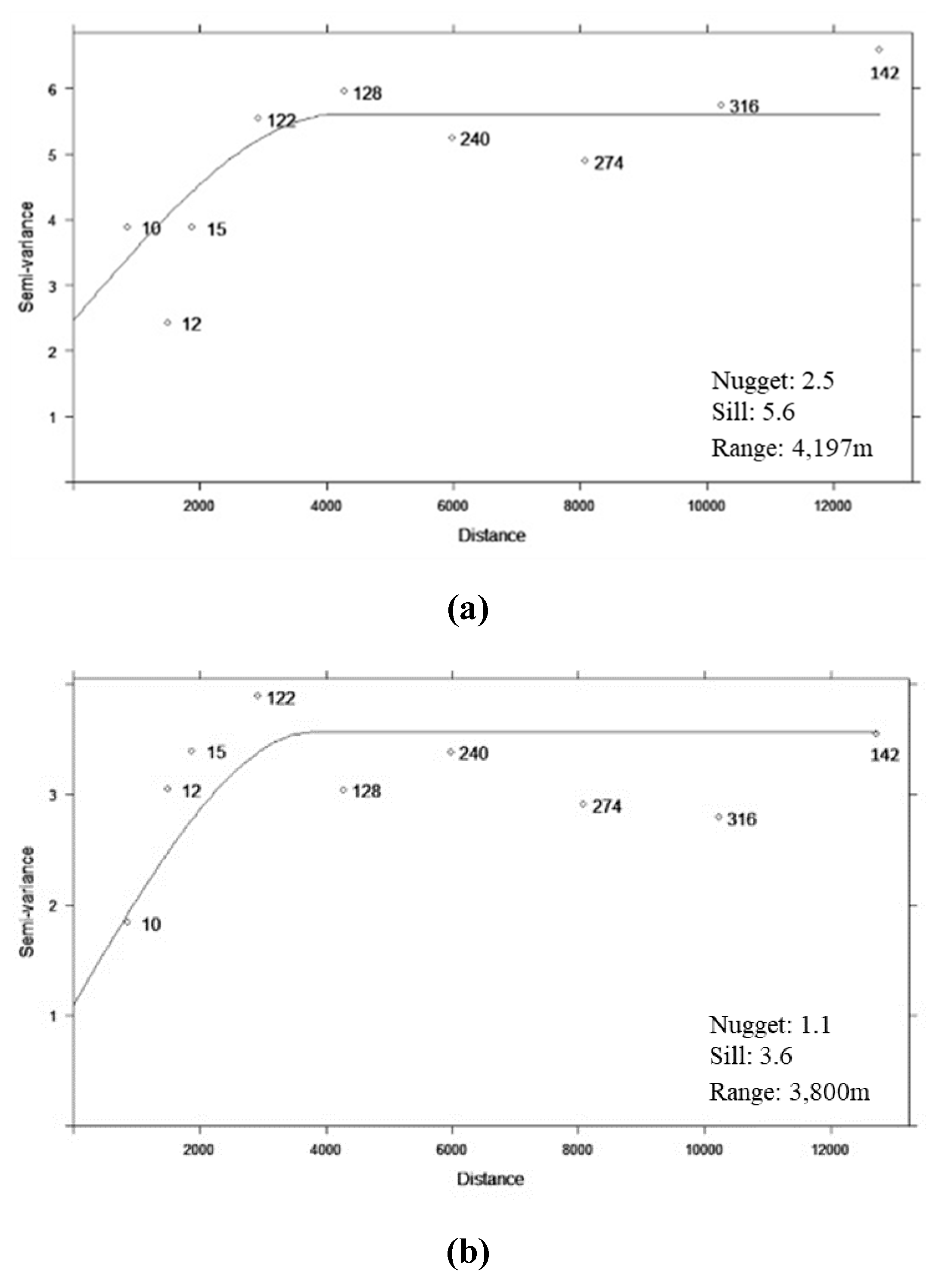
GCPs play a crucial role both for bringing the coordinates of the original orthoimage grid into the desired coordinate system and for assessing the georeferencing final accuracy beside the check points (CPs). In fact, accuracy is assessed determining the mismatch between GCP coordinates before and after the georeferencing stage. During that stage, misalignments propagate from GCPs to nearby locations, favouring the onset of areas characterized by low accuracy (weak areas) [16]. The similarity of error values at neighbouring locations makes evident the spatially auto-correlated nature of coordinate errors. Hence, geostatistics [28,29] appear to be the most suitable theoretical framework to effectively model those errors [30].

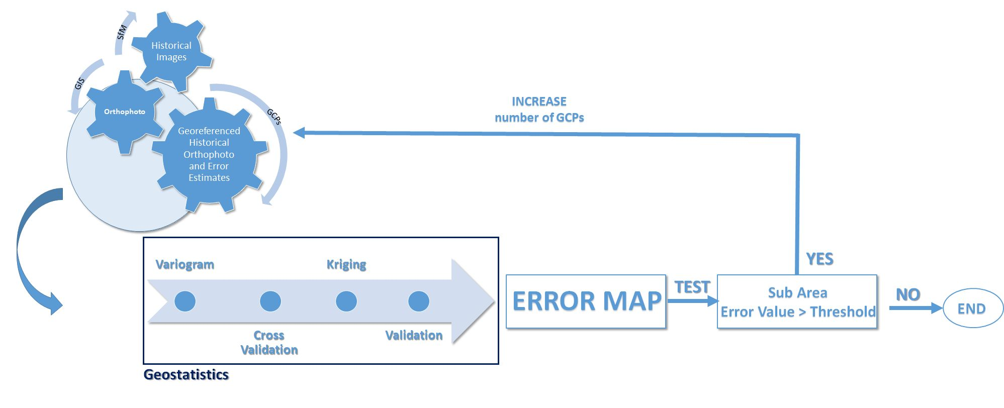
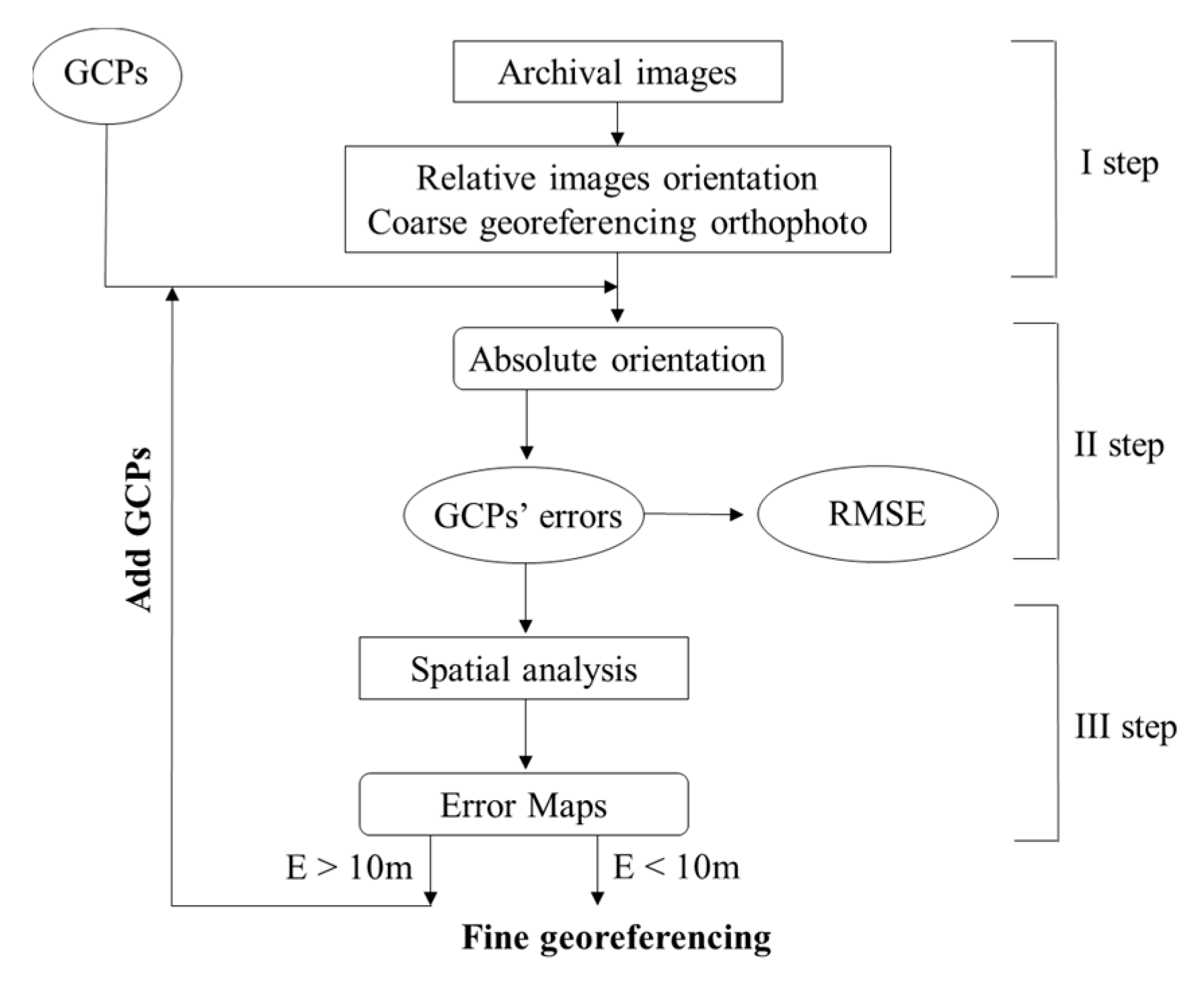
The rationale of the proposed methodology is as follows: at the first stage, a deliberately gross version of the considered orthomosaic is produced by means of a small number of GCPs randomly spread over the study area. GCPs (local) errors, assessed by means of Pix4D software, are then spatialized by use of the kriging interpolator. An error raster map is thus produced, where sub-areas characterized by high local errors can be easily identified. The initial set is then integrated by new GCPs that are placed within or neighbouring such sub-areas. Therefore, the spatial distribution of GCPs is stratified; the first stratum is random, and the second is preferential. The georeferencing procedure is then re-run, and the accuracy of the resulting orthomosaic is assessed once more; if that accuracy is deemed unsatisfactory, GCPs’ errors are re-modelled for re-defining weak areas where new GCPs are placed. That procedure can be repeated as many times as desired until large errors are completely filtered out [31]. In summary, the random distributed stratum is defined at the first stage, once for all, whereas the second stratum can be recursively increased until the desired accuracy is obtained. The effectiveness of the proposed error model is confirmed by [27]. In fact, that paper reports that errors are not indefinitely compressible, but there is a threshold of the GCP number beyond which there is no further improvement in the accuracy. That finding is not particularly surprising because it is actually inherent to the considered theoretical framework. In conclusion, it was shown that the proposed procedure addresses all three open issues mentioned above.

The presented case study concerns the georeferencing of 67 archival AAPs dating back to the 1950s with a desired error threshold of 10 m, which is typical within the forestry scope for large-scale studies. The study results, compared with similar works on archival photographic georeferencing, showed better performance in achieving a final orthomosaic with the same RMSE at a lower information cost computed in terms of nGCPs/km² [18,27,32].

The present study is a follow-up of the QUALIGOUV project (IG-MED 08-392), financed by the European Regional Development Fund, aimed at improving the governance and quality of forest management in protected Mediterranean areas. The proposed methodology was also developed for the ‘Alta Murgia’ National Park (Southern Italy) in order to study the evolution of the reforestations owned by the Puglia region, managed by the A.R.I.F. (Regional Agency for Irrigation and Forestry).

2. Study Area and Data Description

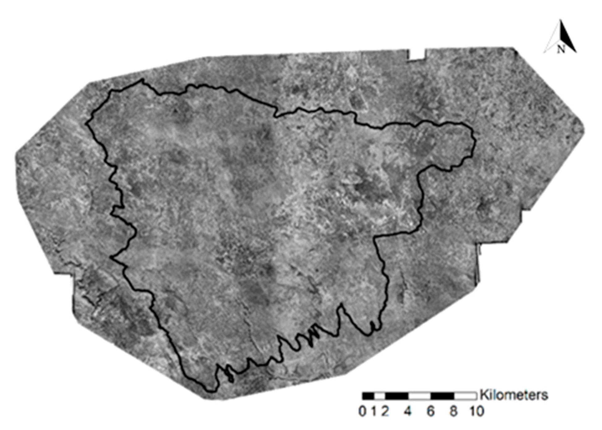
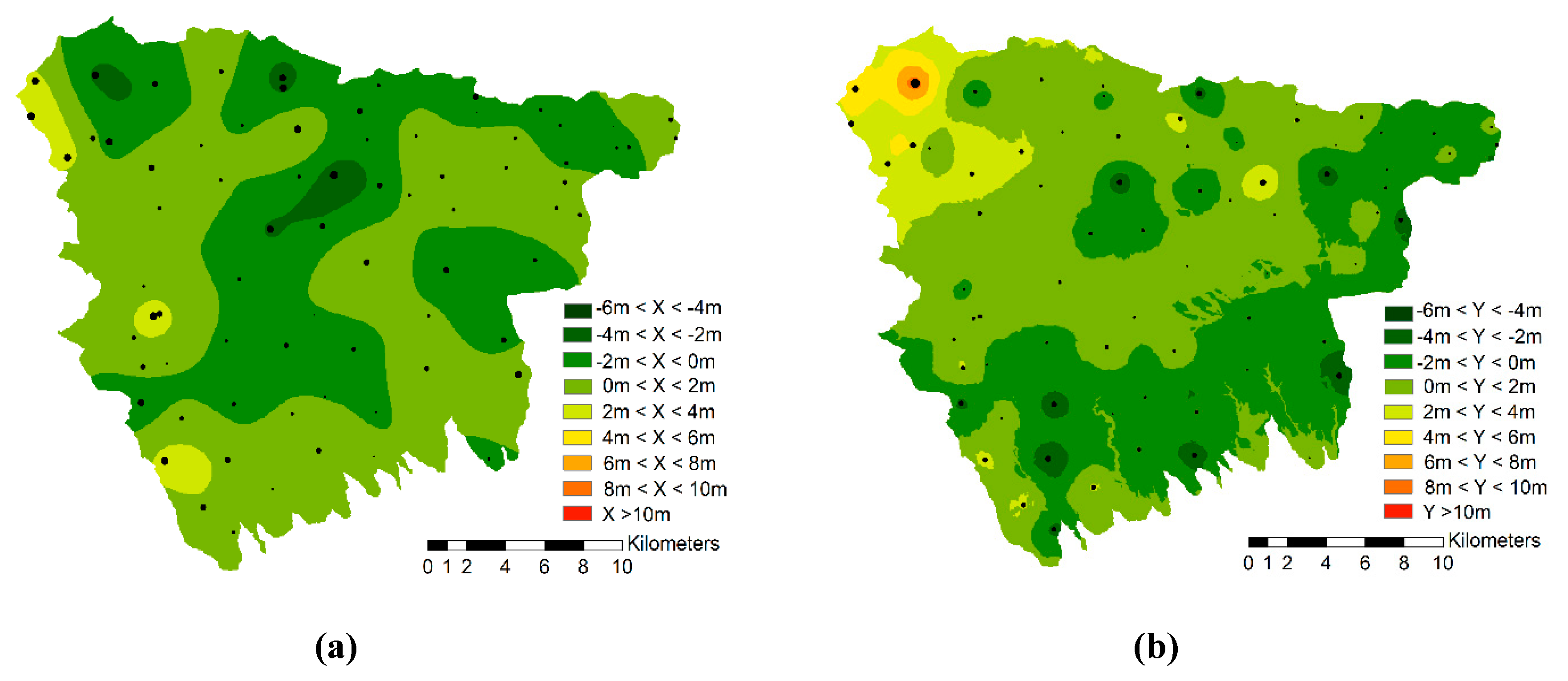
The study area covers a surface of approximately 55,000 ha, and is located on the border between two regions, Puglia and Basilicata, in Southern Italy. It is included in the ‘Murge’, a low limestone plateau dominating the landscape of the central part of the Puglia region. The delineation of the study area was carried out considering the hydrographic basin system of the streams crossing the western part of the Regional Natural Park ‘Terra delle Gravine’.

The area can be divided into three different longitudinal strips that differ in terms of altitude, morphology, land cover, and presence of forest vegetation (Figure 1a).

The northern zone, between 500 and 380 asl, is characterized by hills generally with south- and south-east exposure, where there are forests of Quercus trojana Webb. The central area, between 400 and 220 asl, consists of a slightly wavy plain, used almost everywhere for agricultural crops [33]. The southern zone, between 350 and 160 asl, is morphologically more complex owing to the presence of a series of deep incisions that appear similar to North American canyons [34], termed ‘gravine’ (Figure 1b). The vegetation mainly comprises forest communities characterized by an accentuated physiognomic and compositional heterogeneity [33]. The transects reported in Figure 2 show the inhomogeneity of the study area and the different degrees of morphological complexity of the three zones reported in Figure 1.

The present study was based on 67 AAPs captured in black and white between 1954 and 1955 during the first Italian National Planimetric Survey. The photographs (23 cm × 23 cm) were taken with metric cameras at a height of 6000 m with an acquisition scale of 1:34,000. The analogue AAPs were digitalized by means of an Epson Expression 1640 XL nonphotogrammetric scanner with a resolution of 800 dpi (or equivalently, 31.75 µm). AAPs were purchased already digitalized from the IAGO/IGM retailer (Italian Army Geographical Office/Istituto Geografico Militare). Scanned images had different orientations relative to the original images, and they had an overlap of approximately 60%.

Furthermore, a digital terrain model (DTM) was obtained by merging DTMs of Apulian and Basilicata regions, which have a resolution of 8 m and 5 m, respectively. Digital orthoimages of the 2016 flight for the Puglia region and that of 2013 for the Basilicata region were used. The two orthophotographs have a scale of 1:5000 with a 50 cm pixel resolution.

3. Materials and Methods

3.1. Methodology

The proposed workflow can be divided into three main steps (Figure 3): (i) orthomosaic production and GCP selection; (ii) absolute orthoimage orientation and GCPs’ coordinates error assessment; and (iii) spatial analysis and error map production. Orthomosaic production is described in Section 3.1.1, and GCP selection is outlined in Section 3.1.2. Variables considered for the improvement of the final orthomosaic accuracy (Section 3.1.3) are the coordinate errors along the X and Y directions that were subjected to spatial analysis (Section 3.1.4).

In conclusion, by analyzing the obtained error maps, areas overcoming a given user-threshold are sought (Section 3.1.4). If these areas are found, the GCP number is then increased (Section 3.1.5); otherwise, the final fine georeferenced orthomosaic is gained.

3.1.1. SfM and Orthomosaic Production

The conventional stereo-approach requires information regarding interior and exterior camera orientation, such as focal length, radial distortion, and fiducial marks [7] located at the four angles of each image. In our case, scans lack the required information. The data characteristics resemble those used in [7,20], and the authors of those contributions highlighted that such cases can be successfully managed by means of the structure from motion–multi-view stereo (SfM–MVS) approach. The basic difference between SfM–MVS and classical photogrammetry consists of three aspects: (i) features that can be automatically identified and matched in images at differing scales, viewing angles, and orientations are considered; (ii) the equations used in the algorithm can be solved without information of camera positions or GCPs, although both can be added and used; and (iii) camera calibration can be automatically solved or refined during the process. The SfM–MVS workflow can be summarized in a number of steps, as follows. During the initial processing, a binary descriptor of the SIFT (scale-invariant feature transform) algorithm is used to extract and then match the features from photographs. On the basis of these features and GCPs, (i) an iterative routine of camera self-calibration, (ii) automatic aerial triangulation (AAT), and (iii) BBA to determine and optimize interior and exterior parameters are performed. After initial processing, maximum point cloud densification is carried out, based on multi-view stereo (MVS) [35,36,37,38]. The final processing steps concern the derivation of a digital elevation model (DEM) and the orthomosaic.

The above-mentioned procedure has been implemented in the software Pix4Dmapper [39]; a commercial product that has a primary point of strength of processing large numbers of images without any knowledge of the camera’s calibration parameters [40].

The procedure includes the following steps:

- Image matching

In each image, key points (points of interest characterized by high contrast or particular textures in the images) are automatically recognized and tied together by the software in relation to their neighbourhood characteristics [7], using SfM algorithms. The number of key points depends on the following: (i) the size of the images and (ii) the visual content. At this step, the image size where the key points were searched and extracted was set to ½, whereas the minimum number of key points to search in each image was set at 10,000 to provide more calibrated images.

- Performing bundle adjustment

Using these key points, the AAT and BBA algorithms were performed to recognize the position and orientations of the camera [41]. During this step, the outputs of SfM–MVS are scaled and georeferenced based on GCPs. The 3D point cloud was densified by setting in the software the point density to optimal, which means that every 3D point was calculated for each 4/image scale pixel, and the minimum number of matching among images was set to 2.

- Creation of final orthomosaic

At the end of the three stages of SfM–MVS, the mosaic of AAPs was orthorectified on the basis of the DEM obtained from the photogrammetric process.

3.1.2. GCP Selection

The GCP selection was carried out considering, for the entire study area, initially 50 GCPs that were easily identifiable, such as man-made structures [17], in order to balance the need to obtain an initial gross georeferencing of the orthomosaic and a nearly sufficient points number for geostatistical treatment. The amount of GCPs considered is a medium-low number with respect to that reported in the scientific literature [42,43,44,45,46], because it is related to the local spatial variability of the considered variable, which, for the case at hand, is not excessively large.

GCPs were found manually after a visual comparison between old scanned photographs and present orthoimages, which returned a substantially random GCPs sampling [47] with an initial ratio of 50/550 ~0.1 GCPs/km². The planimetric coordinates of the GCPs (X and Y) were determined in a geographical information system (GIS) using the digital orthophotos, whereas Z coordinates were extrapolated from the DTMs. The reference system used for frame image georeferencing was WGS84/UTM 33N. After the geostatistical analysis, the second stratum of GCPs is selected within the areas characterized by high local errors. In conclusion, the set of GCPs is sampled in a stratified fashion with a first random stratum and a second preferential stratum.

3.1.3. Variables of Interest

The error value at each GCP coordinate (Error X and Error Y) was computed as the difference between the coordinates estimated by Pix4Dmapper in the archival orthomosaic and the real ones identified by the user in a more recent orthophotograph.

In more formal language, an error at a spatial point with coordinates x can be modelled as a sum of two components (1):

$$E\left(x\right)=\eta \left(x\right)+\epsilon \left(x\right), x\in D$$

(1)

where η is the spatially auto-correlated component, ε is the pure random spatially un-correlated component (white noise), and D is the study area [48]. The white noise component represents the uncompressible error, whereas η (auto-correlated error) can be suitably modelled and reduced (filtered out) by adding new GCPs.

Errors in the X and Y directions were selected as variables to be modelled. The variable error Z was not considered during the geostatistical analysis because the study purpose, being oriented to forestry scope, was to assess only the planimetric accuracy of the final orthomosaic. The maximum error (in absolute value) allowed in terms of accuracy was set to 10 m for both the X and Y coordinates. This threshold was considered appropriate by the authors for the purposes of the study.

3.1.4. Spatial Analysis

Spatial analysis scope includes the following:

• statistics for checking the spatial auto-correlation with Moran index;
• techniques to analyze and model (variography) the spatial heterogeneity of the variables of interest;
• methods to perform predictions of considered variables over the study area (kriging) [46].

- Moran Index

The predisposition of the considered variables to be spatialized is commonly checked using Moran’s autocorrelation index (2), which is an extension of the Pearson product–moment correlation coefficient [49]:

$$I=\frac{N}{S_0}\frac{{{\displaystyle \sum }}_{i=1}^N{{\displaystyle \sum }}_{j=1}^N{\omega }_{i,j}{z}_i{z}_j}{{{\displaystyle \sum }}_{i=1}^N{z}_i^2}$$

(2)

where $z_i=\left(x_i-\overline{x}\right)$, $z_j=\left(x_j-\overline{x}\right)$ and $S_0={\displaystyle \sum }_{i=1}^N{\displaystyle \sum }_{j=1}^N{\omega }_{i,j}$

Moran’s index computes a weighted correlation of a variable against itself, where the weights are related to the variable’s spatial arrangement [50].

- Geostatistics

The geostatistical analysis is applied for evaluating the spatial heterogeneity of the considered variables (errors along the Cartesian axis) through the structural analysis (variography) and producing maps by means of spatial prediction methods (kriging).

Variography is a two-stage approach, where a function derived from observations, namely the experimental variogram (the grey dotted line in Figure 4), is used to derive a variogram model (the solid line in Figure 4). This model is the mathematical law ruling the spatial heterogeneity of the considered variable [48].

- Variogram fitting

The computational process from experimental variogram to variogram model is referred to as variogram fitting The selection of the best theoretical model is performed by means of an index of goodness-of-fitting termed $SSErr$, which measures the difference between the discrete experimental variogram and the fitted theoretical model at the same lag value (3):

$$SSErr={\displaystyle \sum }_{i=1}^N\frac{N_i}{h^2{}_i}{\left({\gamma }_{exp}\left(h_i\right)-{\gamma }_{theor}\left(h_i\right)\right)}^2$$

(3)

where ${\gamma }_{theor}\left(i\right)$ is the variogram model value for the distance $h_i$, ${\gamma }_{exp}\left(h_i\right)$ is the analogous value of the experimental variogram, and ${\mathrm{N}}_{\mathrm{i}}$ is the number of point pairs for lag i [51]. The selected model is that having the lowest value of $SSErr$ among all those analyzed during the optimization process.

- Kriging

Variography requires a complementary interpolation method to provide predictions of the variables of interest at unsampled points. The main predictive method in the geostatistical framework is kriging. It is substantially a weighted average, the weights of which are derived from the variogram model. Formula (4) refers to ordinary kriging, which is the most commonly used predictive geostatistical method:

$$\widehat{z}\left({\mathit{s}}_0\right)={\displaystyle \sum }_{i=1}^N{\lambda }_i·z\left({\mathit{s}}_i\right)$$

(4)

where ${\mathit{s}}_0$ is the spatial location associated to the desired prediction, ${\lambda }_i$ are kriging weights, and $z\left({\mathit{s}}_i\right)$ is the observations at the generic location $s_i$. On the basis of its definition, kriging is a best linear unbiased predictor (BLUP) [46]. Afterwards, a spatial map of predictions can be produced.

- Cross-validation and validation stages

Cross-validation and validation are two quite different processes used for model validation. In the first, validation data are the same as those used previously to calibrate the variogram model; whereas in the second case, validation data are different from those used for model calibration.

(Leave-one-out) cross-validation is a procedure in which, given $Z\left(s_i\right)$ a set of n observations at spatial locations $s_i$, the method extracts one observation $Z\left(s_i\right)$ at a time and makes the prediction of that observation, referred to as $\widehat{Z}{\left(s_j\right)}_{-i}$, using the remaining observations (Figure 5).

In the present study, the validation stage was performed using another 25 CPs, selected independently from the GCPs used for the georeferencing. Finally, a scatterplot of the predictions versus the observations can be drawn to determine whether they align along the first quadrant bisector, which would indicate a good capability of the model for capturing the features of the spatial process [48].

- Lin’s concordance index

In general, the agreement between predictions and observations is carried out by means of Pearson or Spearman indices. In the present paper, Lin’s concordance (agreement) coefficient is preferred to quantify the goodness of model adaptation, checking the agreement between observed versus predicted values. Lin’s concordance coefficient provides a measure of overall accuracy that takes into account both bias correction (closeness of the prediction to the actual value) and precision (variability in the predictions). Bias correction is calculated from two bias measures, constant (location-shift) and systematic (scale-shift) bias [52]. The formula as follows (5):

$${\rho }_{c=\frac{2·r·s_X·s_Y}{s_Y^2+s_X^2+{\left(m_{Y }-m_X\right)}^2}}$$

(5)

where $\mathrm{r}$ is the Pearson’s coefficient; $s_X·s_Y$ are the standard deviations of the true and predicted values, respectively; $m_X$ and $m_Y$ are the means; and $s_Y^2$ and $s_X^2$ are the variances of the true and predicted values, respectively.

The R [53,54] libraries used to perform the above mentioned computations were carried out using {RGeostats} [55] and {automap} [51], {Hmisc} [56], and {spdep} [57].

3.1.5. GCP Increasing Strategy

If the local accuracy assessed by means of the kriging maps of error X and error Y shows values above the given threshold, to improve that accuracy, a number of new GCPs will be introduced. The applied strategy to increase the GCP number works as follows:

-

the areas surrounding the worst local errors for error X and error Y maps are delineated;

-

each area is multiplied by the ratio between the initial number of GCPs and the study area size to obtain the number of GCPs to be introduced (0.1 for the case at hand);

-

these new GCPs are located with priority within the weak areas where man-made structures are recognizable, otherwise they are placed in the closest allowed positions.

4. Results

4.1. Stage 1: 50 GCPs

According to the methodology described at the specific section, at the first stage, the orthomosaic with a ground sampling distance (GSD) of 1.73 m. was generated, based on the technical characteristics of the considered photographs (Figure 6).

In the first step, 50 GCPs were randomly selected over the area of interest for georeferencing such an orthomosaic.

4.1.1. Basic Statistics

At the end of the georeferencing process, an error matrix (50 × 3) was provided containing the errors of each GCP (termed error X, error Y, and error Z, respectively) along the (X, Y, Z) axes and three summary RMSE values (

Table 1. Root mean square error (RMSE) values referring to the 50 ground control point (GCP) and 25 check point (CP) dataset.

Variables	Error X	Error Y	Error Z
RMSE (m)—GCP	2.82	3.29	4.84
RMSE (m)—CP	3.56	2.50	6.31

). As already mentioned, only the error X and error Y variables were analyzed; nevertheless, for the sake of completeness, the statistics related to error Z will also be reported at each process stage. From comparison between RMSE from GCPs and CPs, it emerges that the differences are not particularly marked, even if the RMSEs of CPs are generally slightly larger, as expected.

It is noteworthy that all the RMSE values (Table 1) are far below the chosen threshold (10 m), but it should be borne in mind that such an index, being based on an average value, hides possible large local errors. According to such an index, the error Z value appears to be the most uncertain, in contrast to error X. Conversely, the general analysis of GCP errors (

Table 2. Basic statistic of the 50 GCP dataset.

Variables	Minimum	Maximum	Mean	Median	Standard Deviation	Skewness	Kurtosis
	(m)	(m)	(m)	(m)	(m)
Error X	−6.23	11.35	0.21	−0.21	2.84	1.09	3.94
Error Y	−3.84	14.74	0.69	0.41	3.25	2.52	9.21
Error Z	−19.19	14.57	−0.22	−0.22	4.88	−0.93	5.10

) can be helpful in understanding the spatial distribution of the large errors to ensure a final orthomosaic with the desired degree of accuracy over the entire study area.

In fact, from the observation of the extreme (maximum and minimum) values, it can be understood if GCPs errors that overcome the given error threshold exist. In fact, all three maximum values of the considered variables overcome the threshold.

4.1.2. Spatial Analysis

For assessing the extent of weak areas of such high error values, geostatistics provides an effective working environment and tools capable of delineating such areas populated by values above the given threshold.

Because geostatistics requires data Gaussianity, skewness and kurtosis were analyzed. The skewness is always different from zero, indicating an asymmetric shape of the empirical distributions, whereas the analysis of kurtosis values highlights that both the distributions (error X and error Y) have high peaks compared with the normal one, particularly accentuated for the second variable (Table 2). The errors along the Z-axis (error Z) were neglected in the following analysis, as mentioned previously.

The quantile-quantile plots (QQ-plots) corresponding to the considered variables (Figure 7) indicate the presence of some outliers, confirming that the distributions generally depart slightly from Gaussianity; however, it was preferred not to transform the datasets to ease the interpretation of the phenomenon.

Before applying geostatistics, a correlation analysis was carried out to determine whether the variables error X and error Y are correlated with the three coordinates (X, Y, Z). Because such a correlation was found (

Table 3. Correlation matrix and p-value referring to the error values with 50 GCP dataset.

Variables	Correlation			p-Value
	X	Y	Z	X	Y	Z
Error X	−0.42	−0.21	−0.08	0.0024 *	0.1349	0.5837
Error Y	−0.41	0.22	0.20	0.0035 *	0.1201	0.1537
Error Z	0.13	−0.24	−0.27	0.3521	0.0989	0.0547

* symbol beside a p-value indicates that the corresponding correlation value is significantly different from zero.

), it is possible to apply as predictor the universal kriging rather than the ordinary kriging, and consequently produce more accurate maps.

Because the distributions were not Gaussian, the non-parametric Spearman correlation index was computed. For the case at hand, a correlation was found, although not particularly strong, with the X coordinate (Table 3).

Moran’s local autocorrelation index showed a significant predisposition of the errors to be spatialized at different ranges. Error X showed a range of 2500 m (Moran’s index = 0.325), whereas error Y showed a Moran’s index of 0.44 at a range of 3500 m. Therefore, the structural analysis (variography) of these variables was performed, and the experimental and spherical variograms and its main parameters are reported below (Figure 8a,b). The selection of the theoretical models was performed using as the fitness function the lowest value of $SSErr$, which measures 6.3 × 10⁻⁶ for error X and 7.8 × 10⁻⁶ for error Y.

The goodness of fit of the variogram models was checked using the cross-validation and the successive validation stage. The validation was performed using a set of 25 CPs selected independently from the 50 GCPs. The outcomes of this stage are also reported in

Table 4. Cross validation and validation results with the 50 GCP dataset.

Variables	Cross Validation	p-Value	Validation	p-Value
	Overall Accuracy (Lin)		Overall Accuracy (Lin)
Error X	0.78	0.009	0.73	0.36
Error Y	0.90	5.47 × 10−5	0.90	0.84

.

The goodness-of-fit quality of cross-validations can be considered quite satisfactory. Conversely, the validations are not equally good, not because of the value assumed by Lin’s coefficient, but, in fact, owing to its non-significance. The reasons for the low performances of the validation stages can be assumed to be related to different causes. Firstly, a cause can be found in the relatively large extent of the nugget with respect to the sill. In fact, the nugget represents substantially a form of spatially uncorrelated random error that, for the case at hand, impacts adversely on the validation outcomes. Nonetheless, because a correlation structure, although weak, is evident from the variograms (Figure 8a,b), the maps were taken into account, anyway. Secondly, from a purely statistical perspective, the low performances of the validation stage can depend on the number of GCPs (50), which is, probably, too low to be a statistically significant sample of the population. In the following, two maps of errors along X and Y, respectively, are reported (Figure 9).

The produced maps can be considered acceptable because a substantial correspondence can be found between observations and predictions, confirming the overall accuracy of values reported above (Table 4). A quick visual inspection of such maps highlights the presence of weak areas that overcome the given error threshold (10 m). The percentage size of such inaccurate areas is 0.21% for error X and 2.53% for error Y, corresponding to approximately 114.5 ha and 1377 ha of the total study area, respectively. The largest errors are located in the north-west and southern parts of the considered maps. Such errors can be related to the poor quality of the archival photographs, leading to increased uncertainty in the choice of points and to an edge effect. The final result highlights that the orthomosaic accuracy cannot be considered completely satisfying for the purpose of the study; hence, it was necessary to increase the number of GCPs, the location of which was suggested by the two error maps.

4.2. Stage 2: 75 GCPs

For the case at hand, 25 new GCPs were introduced following the methodology outlined in Section 3.1.5. The number of GCPs was achieved by summing the weak areas’ sizes of error X and error Y, approximately 250 km², and multiplying that value by 0.1; that is, the ratio between the initial number of GCPs and the entire study area size (see Section 3.1.2). The placement of the new GCPs was pursued by seeking man-made structures over or close to weak areas; hence, such additional sampling is preferential. In Figure 10, the spatial distribution over the two errors maps of the 25 GCPs just introduced are reported.

4.2.1. Basic Statistics

Once identified, the GCPs were added to the dataset, and the georeferencing of the orthomosaic was repeated, producing an error matrix of 75 × 3.

The results of the RMSE values are shown in

Table 5. RMSE values referring to the 75 GCP and 25 CP dataset.

Variables	Error X	Error Y	Error Z
RMSE (m)—GCP	2.42	2.24	3.32
RMSE (m)—CP	3.08	2.54	4.66

.

The table shows that the RMSEs of GCPs values related to error X and error Y decreased (13.94% and 31.87%, respectively), but as already noted, the analysis of such a parameter is insufficient to establish the absence of weak areas. The RMSE related to error X improved by 13.55%, confirming the improvement of RMSE of GCPs. The RMSE related to error Y showed a worsening of 1.35%.

Therefore, a statistical analysis of GCPs was performed once more.

The basic statistics referring to the errors of the three coordinates of the GCPs highlight a noticeable improvement characterized by the decrease in absolute terms of the extreme values (minimum and maximum) (

Table 6. Basic statistic of the 75 GCP dataset.

Variables	Minimum	Maximum	Mean	Median	Standard Deviation	Skewness	Kurtosis
	(m)	(m)	(m)	(m)	(m)
Error X	−5.59	5.08	0.18	0.38	2.43	−0.08	−0.33
Error Y	−3.82	9.26	0.32	0.41	2.24	0.79	2.38
Error Z	−7.20	8.50	0.16	0.12	3.34	0.03	0.56

).

The QQ-plots, skewness, and kurtosis of error X and error Y variables (Figure 11) show a distribution closer to a Gaussian one, with the exception of error Y, which still has outlier values, but they were lower than the threshold.

4.2.2. Stage 1 vs. Stage 2

Given the peculiar methodology structure, the values of the first 50 GCP errors at this stage can be compared with the values of the same GCPs at the previous stage.

It can be demonstrated that the worst values (minimums and maximums) had improved significantly after the increase of the GCPs, as reported in

Table 7. Fifty GCP stage 1 vs. 50 GCP stage 2.

Variables	Minimum	Maximum	Mean
	(%)	(%)	(%)
Error X	−28.54	−58.62	−107.93
Error Y	−0.60	−37.20	−90.94
Error Z	−114.33	−41.61	−260.54

.

In more detail, such an analysis can be broadened to check how many points have improved and how many worsened and to what extent they were changed (Figure 12).

Table 8. Improvement and worsening of the first 50 GCPs compared with the first and second steps.

Variables	GCPs Improved	GCPs Worsened	Improvement Mean	Worsening Mean
	n.	n.	(m)	(m)
Error X	22	28	1.15	−0.45
Error Y	28	22	0.95	−0.50
Error Z	33	17	1.85	−1.21

summarizes the results in Figure 12 for all variables.

Concerning error X, the result can seem poor in absolute terms because the number of improvements is less than that of worsening. However, when examining the average values related to the improvements and worsening, it is clear that the average improvements outperform the worsening by approximately threefold. Hence, worsening, when it takes place, can be considered to be practically negligible.

Concerning the error Y results, in this case, the number of improvements overcomes the number of worsening and, once more, the average intensity of the improvement outperforms by about two times the worsening. The comparison of the standard deviation values indicates a tendency to decrease. The error X value goes from 2.84 to 2.22 m; error Y from 3.25 to 2.34 m; and, in particular, the error Z value decreases from 4.88 to 3.25 m. This result indicates that, in general, the model equalizes the error values, making them more similar to each other in this second step than in the first one.

4.2.3. Spatial Analysis

The most relevant result is that both error X and error Y present no more local values that overcome the given threshold. Hence, the addition of a further 25 points enables the desired goal to be achieved, and the spatial analysis was performed anyway to compare the maps obtained by 50 and 75 GCPs. As noted previously, the correlation analysis between the variables and coordinates was performed. From

Table 9. Correlation matrix and p-value referring to error values with the 75 GCP dataset.

Variables	Correlation			p-Value
	X	Y	Z	X	Y	Z
Error X	−0.18	−0.20	−0.12	0.1306	0.0846	0.2904
Error Y	−0.39	0.25	0.21	0.0006 *	0.0282 *	0.0682 *
Error Z	−0.07	−0.15	−0.13	0.5357	0.2097	0.2734

* symbol beside a p-value indicates that the corresponding correlation value is significantly different from zero.

, it can be seen that error Y is correlated significantly to all three coordinates. The other two errors do not present any significant correlation.

Moran’s local index indicated a spatial autocorrelation at lower ranges compared with the previous step; error X and error Y have a range of 1500 m (Moran’s index = 0.48) and 2000 m (Moran’s index = 0.31), respectively, indicating that a part of the structural error was filtered out after new GCPs addition. The spherical model reported lower values of $SSErr$ 2.7 × 10⁻⁵ for error X and 6.5 × 10⁻⁶ for error Y, highlighting a clear improvement of the variograms, the parameters and goodness of fit indices of which are reported in Figure 13.

Table 10. Cross validation and validation results with the 75 GCP dataset.

Variables	Cross Validation	p-Value	Validation	p-Value
	Overall Accuracy (Lin)		Overall Accuracy (Lin)
Error X	0.56	0.009	0.53	0.00
Error Y	0.85	7.53 × 10−6	0.82	0.03

reports the overall accuracies related to cross validation and validation stages. Error X shows an accuracy that is nearly sufficient, whereas error Y shows accuracy values that are quite satisfactory.

An explanation for such different behaviour can be tied to the selection of the 25 new points; they lowered the structural part of error X, whereas error Y was only impacted negligibly. This difference may be owing to a different uncertainty degree related to the X coordinate (uncompressible error) with respect to the Y coordinate (auto-correlated error).

Finally, two maps of errors along X and Y, respectively, were reported (Figure 14).

By analyzing both maps, it can be observed that, after using 75 GCPs for georeferencing the orthomosaic, some residual weak areas with high error values are located approximately at the same positions (Error Y map); however, in absolute terms, the error values are far below those at the earlier stage.

5. Discussion

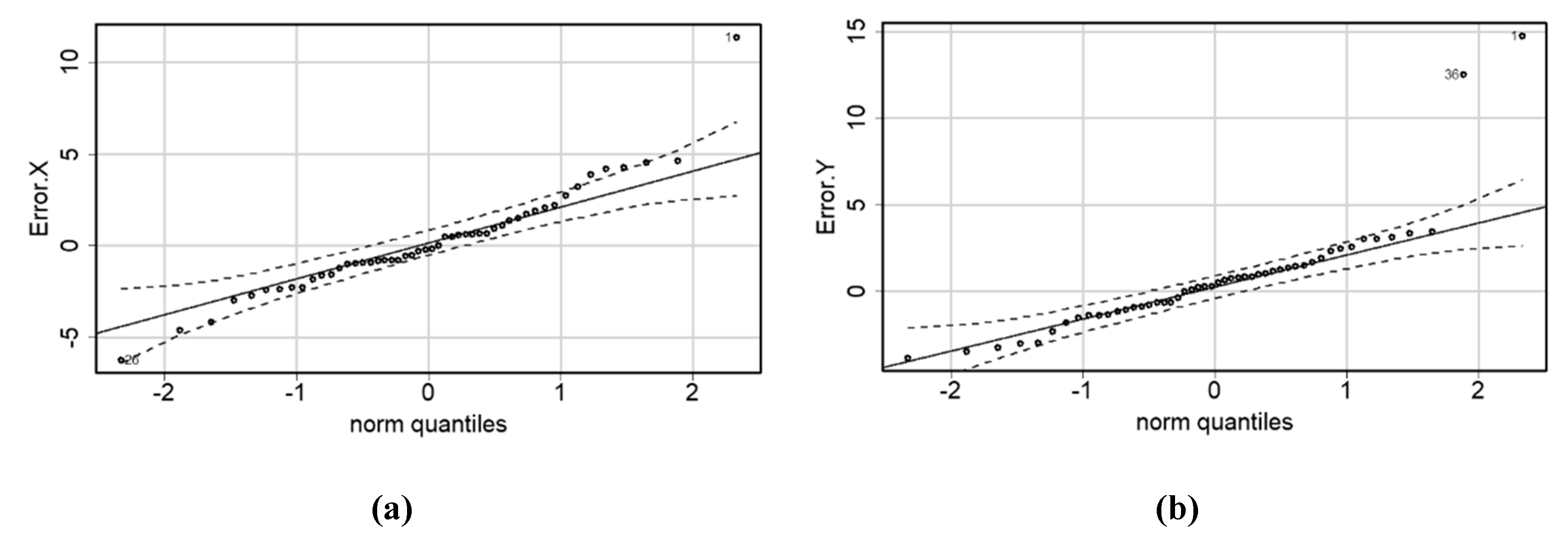
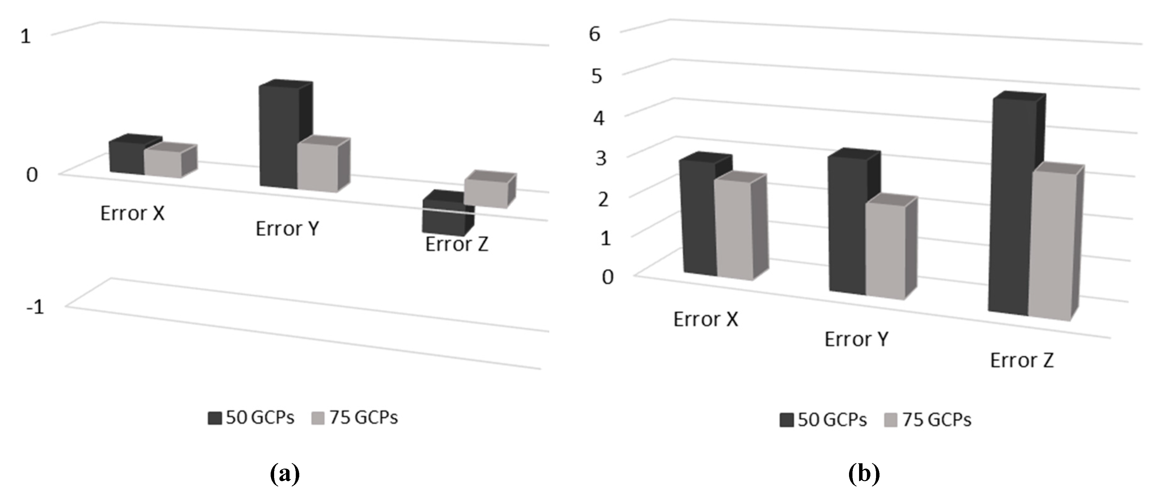
Figure 15a shows the variation of the mean values related to the three errors before and after the application of the proposed methodology. As a first remark, it is noticeable that the mean values were reduced and tend to zero. Another feature of this result is the sign of the mean value that is positive after the methodology application, which suggests that there is a tendency to overestimate the error values during the kriging application. 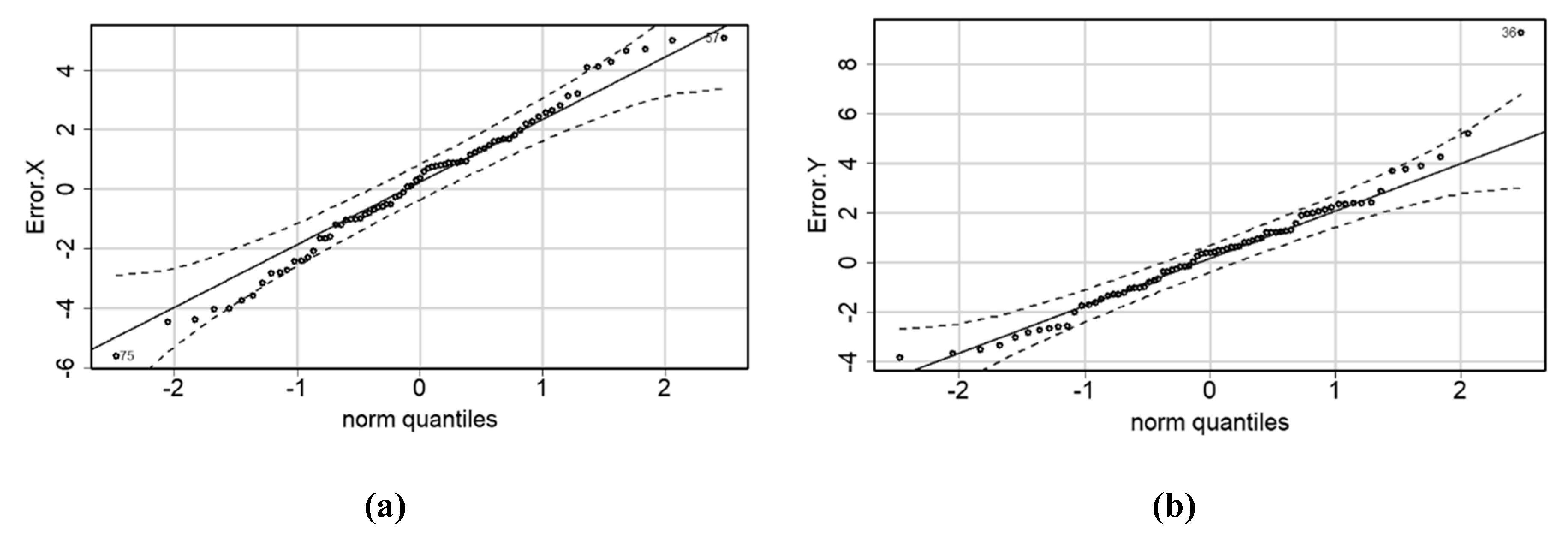Concerning Figure 15b, a decrease in the standard deviation values is apparent. An interpretation of this result is that a tendency exists towards an equalization of the error values; that is to say, the structural error vanishes, and the white noise remains, as expected. In fact, the three error distributions become even more similar to the general white noise distribution that is Gaussian centred on zero.

To provide a judgement regarding the appropriateness of this methodology, it is necessary to compare the achieved results with the existing literature. After a review, it emerged that authors typically tend to lower RMSE values and achieve a fine georeferencing using a large information rate for unit area (ratio between number of GCPs and the size of the study area), which can be measured as nGCPs/Km² [18,32] (see

Table 11. Comparison between the present study and the literature.

	Area Surface	Archival Images	GCPs	nGCPs/Km2	RMSE Mean
	(km2)	(n)	(n)		(m)
Present study	550	67	50	0.09	3.65
Present study	550	67	75	0.13	2.66
[1] Vuorela et al., 2002	9	-	108	12	4.80
[7] Molg and Bolch, 2017	16	7	24	1.5	4.88
[18] Martínez-Carricondo et al., 2018	0.18	160	20	113.38	0.048
[21] Gonçalves, 2016	0.3	24	8	26.67	4.7
[25] Micheletti, et al., 2015	20	12	169	8.45	0.34
[27] Oniga et al., 2020	0.08	-	150	1.87	2.1

). Hence, there is a general tendency for neglecting the GCPs’ positions in favour of their number.

The issue of minimizing the GCP number optimally has been addressed by many authors. Table 11 reports the results derived from a set of papers, the contributions of which can be grouped into three main categories: (i) the use of archival aerial photogrammetry to quantify the landscape change [1,25]; (ii) the application of SfM for orientation, orthorectification, and mosaic composition of historical aerial images [7,21]; and (iii) the optimal distribution [18] and number [27] of GCPs to optimize the accuracy of the georeferencing process obtained by unmanned aerial vehicle (UAV) photogrammetry.

Table 11 demonstrates clearly that, by comparing results from the scientific literature with those achieved in the present paper, it is, in fact, possible to reach the same RMSE values with a reduced information rate for area unit. This was reached by selecting GCPs in the areas highlighted during the geostatistical analysis (weak areas).

Therefore, this finding demonstrates that GCP position can be a key piece of information for achieving a fine georeferencing as much as the GCP number. In Table 11, the references reporting a better result compared with the present study are those of [25,27] and [18]. However, it should be highlighted that the nGCPs/Km² is approximately 65, 10, and 871 times larger than the results obtained here, and the corresponding size areas are substantially smaller than the presented study area. It may be that it would have been possible to achieve a similar goal with a smaller increase in the information rate, but such an analysis was beyond the objective of the present study.

Another important result is that the optimal (minimal) number of GCPs required to achieve the study’s main objective is within the range of 50 < opt ≤ 75. Furthermore, it is noticeable that the RMSE related to error Z improved strongly, notwithstanding the fact the GCPs were selected with respect to errors X and Y only. This association suggests the possible existence of inter-relationships between the three errors and that, probably, an improvement along a single direction can impact positively upon all the remaining errors. Therefore, applying the methodology to a single direction could achieve similar results in terms of accuracy by simplifying the overall complexity of the procedure to a significant degree.

From a computational standpoint, it can be stated that the proposed methodology converged after only a single run for the presented case study. This is not surprising, because simulation trials demonstrated that, at most, a couple of runs are sufficient to reach the desired accuracy. Therefore, the methodology is generally also particularly rapid.

6. Conclusions

This research has presented a geostatistically-based methodology aimed at the following: (i) assessing and mapping the local accuracy of a grossly georeferenced archival orthomosaic; and (ii) improving that accuracy to meet a given error threshold (10 m) by selecting a number of GCPs within or close to areas affected by large errors [16] reported by error maps.

After the methodology’s application, (i) the target error was, in fact, reached along all three axes, and (ii) the target was reached with a minimal quantity of GCPs. The (ii) point was gained not by chance, but as an effect of limiting areas within which GCPs were found.

To compare two different GCP configurations over two different areas, the information rate per unit area, measured in terms of nGCPs/Km², can be an effective index.

A review reported in Table 11 shows that the rate was substantially lower than those considered in this study. To test the proposed methodology, a wide and morphologically complex study area was considered. The methodology found the convergence towards a satisfying solution after only one run. The results showed a significant improvement for error X, which decreased far below the given threshold; in fact, the largest local error was approximately 5 m, only half of the required target. The same large positive impact was found for error Z, notwithstanding the fact that the GCP selection strategy was not driven by such a variable. At first sight, error Y, observing the behaviour of the largest errors, would appear to be influenced in a lower measure by the proposed procedure, but this impression is incorrect because the RMSE improved by approximately 32%. In addition, as emerged following the geostatistical analysis, the structural error was not completely filtered out [31], demonstrating potential room for further improvement. However, because the largest errors decreased below the given threshold (even if by only a small amount), and the local errors converged towards a uniform value over the entire study area, the procedure was stopped.

Therefore, the procedure can be considered validated and the application fully successful. Regarding the next developments, we consider that the addressed topic deserves further investigation. In particular, research into the error propagation during georeferencing process is presently in progress. The initial results are interesting and are likely to be of high significance.

References

1. Vuorela, N.K.; Alho, P.; Kalliola, R. Systematic Assessment of Maps as Source Information in Landscape-change Research. Landsc. Res. 2002, 27, 141–166. [Google Scholar] [CrossRef]
2. Redweik, P.; Roque, D.; Marques, A.; Matildes, R.; Marques, F. Triangulating the Past—Recovering Portugal’s Aerial Images Repository. Photogramm. Eng. Remote Sens. 2010, 76, 1007–1018. [Google Scholar] [CrossRef]
3. Mojses, M.; Petrovič, F. Land use changes of historical structures in the agricultural landscape at the local level—Hriňová case study. Ekologia 2013, 32, 1–12. [Google Scholar] [CrossRef] [Green Version]
4. Frankl, A.; Seghers, V.; Stal, C.; de Maeyer, P.; Petrie, G.; Nyssen, J. Using image-based modelling (SfM–MVS) to produce a 1935 ortho-mosaic of the Ethiopian highlands. Int. J. Digit. Earth 2014, 8, 421–430. [Google Scholar] [CrossRef] [Green Version]
5. Lallias-Tacon, S.; Liébault, F.; Piégay, H. Use of airborne LiDAR and historical aerial photos for characterising the history of braided river floodplain morphology and vegetation responses. Catena 2017, 149, 742–759. [Google Scholar] [CrossRef]
6. San-Antonio-Gómez, C.; Velilla, C.; Manzano-Agugliaro, F. Urban and landscape changes through historical maps: The Real Sitio of Aranjuez (1775–2005), a case study. Comput. Environ. Urban Syst. 2014, 44, 47–58. [Google Scholar] [CrossRef]
7. Mölg, N.; Bolch, T. Structure-from-Motion Using Historical Aerial Images to Analyse Changes in Glacier Surface Elevation. Remote Sens. 2017, 9, 1021. [Google Scholar] [CrossRef] [Green Version]
8. del Soldato, M.; Riquelme, A.; Bianchini, S.; Tomas, R.; di Martire, D.; de Vita, P.; Moretti, S.; Calcaterra, D. Multisource data integration to investigate one century of evolution for the Agnone landslide (Molise, southern Italy). Landslides 2018, 15, 2113–2128. [Google Scholar] [CrossRef] [Green Version]
9. Cencetti, C.; di Matteo, L.; Romeo, S. Analysis of Costantino Landslide Dam Evolution (Southern Italy) by Means of Satellite Images, Aerial Photos, and Climate Data. Geosciences 2017, 7, 30. [Google Scholar] [CrossRef] [Green Version]
10. Notti, D.; Galve, J.P.; Mateos, R.M.; Monserrat, O.; Lamas-Fernández, F.; Fernández-Chacón, F.; Roldán-García, F.J.; Pérez-Peña, J.V.; Crosetto, M.; Azañón, J.M. Human-induced coastal landslide reactivation. Monitoring by PSInSAR techniques and urban damage survey (SE Spain). Landslides 2015, 12, 1007–1014. [Google Scholar] [CrossRef]
11. Ma, R.; Broadbent, M.; Zhao, X. Historical Photograph Orthorectification Using SfM for Land Cover Change Analysis. J. Indian Soc. Remote Sens. 2019, 48, 341–351. [Google Scholar] [CrossRef]
12. Cléri, I.; Pierrot-Deseilligny, M.; Vallet, B. Automatic Georeferencing of a Heritage of old analog aerial Photographs. ISPRS Ann. Photogramm. Remote Sens. 2014, 33–40. [Google Scholar] [CrossRef] [Green Version]
13. Nurminen, K.; Litkey, P.; Honkavaara, E.; Vastaranta, M.; Holopainen, M.; Lyytikäinen-Saarenmaa, P.; Kantola, T.; Lyytikäinen, M. Automation Aspects for the Georeferencing of Photogrammetric Aerial Image Archives in Forested Scenes. Remote. Sens. 2015, 7, 1565–1593. [Google Scholar] [CrossRef] [Green Version]
14. Nocerino, E.; Menna, F. Multi-temporal analysis of landscapes and urban areas. Int. Arch. Photogramm. 2012, 85–90. [Google Scholar] [CrossRef] [Green Version]
15. Necsoiu, M.; Dinwiddie, C.; Walter, G.R.; Larsen, A.; Stothoff, S. Multi-temporal image analysis of historical aerial photographs and recent satellite imagery reveals evolution of water body surface area and polygonal terrain morphology in Kobuk Valley National Park, Alaska. Environ. Res. Lett. 2013, 8, 025007. [Google Scholar] [CrossRef] [Green Version]
16. Aguilar, M.A.; Aguilar, F.J.; Fernández, I.; Mills, J.; Torres, M. Ángel A. Accuracy Assessment of Commercial Self-Calibrating Bundle Adjustment Routines Applied to Archival Aerial Photography. Photogramm. Rec. 2012, 28, 96–114. [Google Scholar] [CrossRef]
17. Giordano, S.; le Bris, A.; Mallet, C. Toward automatic georeferencing of archival aerial photogrammetric surveys. ISPRS Ann. Photogramm. Remote Sens. 2018, 4, 105–112. [Google Scholar] [CrossRef] [Green Version]
18. Carricondo, P.J.M.; Vega, F.A.; Carvajal-Ramirez, F.; Mesas-Carrascosa, F.-J.; García-Ferrer, A.; Pérez-Porras, F.-J. Assessment of UAV-photogrammetric mapping accuracy based on variation of ground control points. Int. J. Appl. Earth Obs. Geoinf. 2018, 72, 1–10. [Google Scholar] [CrossRef]
19. Verhoeven, G.; Taelman, D.; Vermeulen, F. Computer vision-based orthophoto mapping of complex archaeological sites: The ancient quarry of Pitaranah (Portugal-Spain). Archaeometry 2012, 54, 1114–1129. [Google Scholar] [CrossRef]
20. Bakker, M.; Lane, S.N. Archival photogrammetric analysis of river-floodplain systems using Structure from Motion (SfM) methods. Earth Surf. Process. Landforms 2016, 42, 1274–1286. [Google Scholar] [CrossRef] [Green Version]
21. Gonçalves, J.A. Automatic orientation and mosaicking of archived aerial photography using structure from motion. Int. Arch. Photogramm. Remote Sens. Spatial Inf. Sci. 2016, 3, 123–126. [Google Scholar] [CrossRef]
22. Willmott, C.; Matsuura, K. Advantages of the mean absolute error (MAE) over the root mean square error (RMSE) in assessing average model performance. Clim. Res. 2005, 30, 79–82. [Google Scholar] [CrossRef]
23. Willmott, C.J.; Matsuura, K.; Robeson, S.M. Ambiguities inherent in sums-of-squares-based error statistics. Atmosph. Environ. 2009, 43, 749–752. [Google Scholar] [CrossRef]
24. Ayoub, F.; Leprince, S.; Avouac, J.-P. Co-registration and correlation of aerial photographs for ground deformation measurements. ISPRS J. Photogramm. Remote Sens. 2009, 64, 551–560. [Google Scholar] [CrossRef]
25. Micheletti, N.; Lane, S.N.; Chandler, J. Application of archival aerial photogrammetry to quantify climate forcing of alpine landscapes. Photogramm. Rec. 2015, 30, 143–165. [Google Scholar] [CrossRef]
26. Giordano, S.; le Bris, A.; Mallet, C. Fully automatic analysis of archival aerial images status and challenges. In Proceedings of the 2017 Joint Urban Remote Sensing Event (JURSE), Dubai, UAE, 6–8 March 2017; pp. 1–4. [Google Scholar] [CrossRef]
27. Oniga, V.-E.; Breaban, A.-I.; Pfeifer, N.; Chirila, C. Determining the Suitable Number of Ground Control Points for UAS Images Georeferencing by Varying Number and Spatial Distribution. Remote. Sens. 2020, 12, 876. [Google Scholar] [CrossRef] [Green Version]
28. Matheron, G. Principles of geostatistics. Econ. Geol. 1963, 58, 1246–1266. [Google Scholar] [CrossRef]
29. Barca, E.; Castrignanò, A.; Ruggieri, S.; Rinaldi, M. A new supervised classifier exploiting spectral-spatial information in the Bayesian framework. Int. J. Appl. Earth Obs. Geoinf. 2020, 86, 101990. [Google Scholar] [CrossRef]
30. Tobler, T.A. Computer Movie Siulating Urban Growth in the Detroit Region. Econ. Geogr. 1970, 46, 234–240. [Google Scholar] [CrossRef]
31. Barca, E.; de Benedetto, D.; Stellacci, A.M. Contribution of EMI and GPR proximal sensing data in soil water content assessment by using linear mixed effects models and geostatistical approaches. Geoderma 2019, 343, 280–293. [Google Scholar] [CrossRef]
32. Siqueira, H.L.; Marcato, J.; Matsubara, E.T.; Eltner, A.; Colares, R.A.; Santos, F.M.; Junior, J.M. The Impact of Ground Control Point Quantity on Area and Volume Measurements with UAV SFM Photogrammetry Applied in Open Pit Mines. In Proceedings of the IGARSS 2019 IEEE International Geoscience and Remote Sensing Symposium, Yokohama, Japan, 28 July–2 August 2019; Institute of Electrical and Electronics Engineers (IEEE): Piscataway, NJ, USA, 2019; pp. 9093–9096. [Google Scholar]
33. Greco, R. Frammentazione Delle Comunità Forestali ed eEerogeneità Ambientale: Il Caso del Parco Naturale Regionale Terra delle Gravine. Ph.D. Thesis, University of Bari, Bari, Italy, 2012. [Google Scholar]
34. Marchant, B.; Lark, R.M. Optimized Sample Schemes for Geostatistical Surveys. Math. Geol. 2007, 39, 113–134. [Google Scholar] [CrossRef]
35. Ullman, S. The interpretation of structure from motion. Proc. R. Soc. Lond. B. 1979, 203, 405–426. [Google Scholar] [CrossRef] [PubMed]
36. Robertson, D.P.; Cipolla, R. Structure from motion. In Practical Image Processing and Computer Vision; Varga, M., Ed.; Wiley: New York, NY, USA, 2009. [Google Scholar]
37. Westoby, M.J.; Brasington, J.; Glasser, N.; Hambrey, M.; Reynolds, J. ‘Structure-from-Motion’ photogrammetry: A low-cost, effective tool for geoscience applications. Geomorphology 2012, 179, 300–314. [Google Scholar] [CrossRef] [Green Version]
38. Verhoeven, G.; Sevara, C.; Karel, W.; Ressl, C.; Doneus, M.; Briese, C. Undistorting the Past: New Techniques for Orthorectification of Archaeological Aerial Frame Imagery. In The Archaeometallurgy of Copper; Springer Science and Business Media LLC: Berlin/Heidelberg, Germany, 2013; pp. 31–67. [Google Scholar]
39. Pix4Dmapper 4.1. User Manual; Pix4D SA: Lausanne, Switzerland, 2017.
40. Broadbent, M. Reconstructing the Past in 3D Using Historical Aerial Imagery. Ph.D. Thesis, University of Redlands, Redlands, CA, USA, 2017. [Google Scholar]
41. Daponte, P.; de Vito, L.; Mazzilli, G.; Picariello, F.; Rapuano, S. A height measurement uncertainty model for archaeological surveys by aerial photogrammetry. Measurement 2017, 98, 192–198. [Google Scholar] [CrossRef]
42. Watson, G.S.; Journel, A.G.; Huijbregts, C.J. Mining Geostatistics. J. Am. Stat. Assoc. 1980, 75, 245. [Google Scholar] [CrossRef]
43. Rutter, C.M.; Isaaks, E.H.; Srivastava, R.M. An Introduction to Applied Geostatistics. J. Am. Stat. Assoc. 1991, 86, 548. [Google Scholar] [CrossRef]
44. Stein, M.L.; Chilès, J.-P.; Delfiner, P. Geostatistics: Modeling Spatial Uncertainty. J. Am. Stat. Assoc. 2000, 95, 335. [Google Scholar] [CrossRef]
45. Wackernagel, H. Multivariate Geostatistics; Springer Science and Business Media LLC: Berlin/Heidelberg, Germany, 2003. [Google Scholar]
46. Webster, R.; Oliver, M.A. Geostatistics for Environmental Scientists; Wiley: New York, NY, USA, 2007. [Google Scholar]
47. de Gruijter, J.J.; Bierkens, M.F.P.; Brus, D.J.; Knotters, M. Sampling for Natural Resource Monitoring; Springer Science and Business Media LLC: Berlin/Heidelberg, Germany, 2006. [Google Scholar]
48. Barca, E.; Porcu, E.; Bruno, D.; Passarella, G. An automated decision support system for aided assessment of variogram models. Environ. Model. Softw. 2017, 87, 72–83. [Google Scholar] [CrossRef]
49. Moran, P.A.P. Notes on Continuous Stochastic Phenomena. Biometrika 1950, 37, 17. [Google Scholar] [CrossRef]
50. Rura, M.J.; Griffith, D.A. Spatial Statistics in SAS. In Handbook of Applied Spatial Analysis; Fischer, M., Getis, A., Eds.; Springer: Berlin/Heidelberg, Germany, 2010. [Google Scholar]
51. Hiemstra, P.H.; Pebesma, E.; Twenhofel, C.J.; Heuvelink, G.B. Real-time automatic interpolation of ambient gamma dose rates from the Dutch radioactivity monitoring network. Comput. Geosci. 2009, 35, 1711–1721. [Google Scholar] [CrossRef]
52. Barnhart, H.X.; Haber, M.; Song, J. Overall concordance correlation coefficient for evaluating agreement among multiple observers. Biometrika 2002, 58, 1020–1027. [Google Scholar] [CrossRef] [PubMed]
53. Development Core Team. R: A Language and Environment for Statistical Computing; R Foundation for Statistical Computing: Vienna, Austria, 2008. [Google Scholar]
54. RStudio Team. RStudio: Integrated Development for R; RStudio, Inc.: Boston, MA, USA, 2015. [Google Scholar]
55. Renard, D.; Bez, N.; Desassis, N.; Beucher, H.; Ors, F.; Laporte, F. RGeostats: The Geostatistical Package; Version 11.0.2; MINES Paris Tech: Paris, France, 2016. [Google Scholar]
56. Harrell, F.E., Jr. Package ‘Hmisc’. CRAN. 2019, pp. 235–236. Available online: https://cran.r-project.org/web/packages/Hmisc/Hmisc.pdf (accessed on 6 April 2020).
57. Bivand, R.; Piras, G. Comparing Implementations of Estimation Methods for Spatial Econometrics. J. Stat. Softw. 2015, 63. [Google Scholar] [CrossRef] [Green Version]
Figure 1. The study area localized in Southern Italy: (a) division of the area into three longitudinal strips. The red line indicates the edge of the study area; (b) Gravina of Laterza (Taranto, Southern Italy).
Remotesensing 12 02232 g001
Figure 2. Elevation sections of the study area from northern (a), central (b), and southern (c) zones.
Remotesensing 12 02232 g002aRemotesensing 12 02232 g002b
Figure 3. Methodology workflow. GCP, ground control point; RMSE, root mean square error.
Remotesensing 12 02232 g003
Figure 4. Experimental and variogram model with corresponding parameters. The total sill ( σ 2 ) corresponds to the sum of the nugget effect and partial sill (the maximum variability degree of the process); the range (α) can be interpreted as the distance beyond which the spatial correlation becomes negligible [48].
Remotesensing 12 02232 g004
Figure 5. Cross validation workflow.
Remotesensing 12 02232 g005
Figure 6. Orthomosaic generated by 67 historical aerial photographs (1954–1955). The black line indicates the study area.
Remotesensing 12 02232 g006
Figure 7. QQ-plots corresponding to the variables calculated with the 50 GCP dataset: (a) error X; (b) error Y.
Remotesensing 12 02232 g007
Figure 8. Experimental variogram and fitted variogram model with the 50 GCP dataset: (a) error X; (b) error Y.
Remotesensing 12 02232 g008
Figure 9. Error maps along the two axes. (a) Error X; (b) error Y. The black points indicate the 50 GCP dataset. The size of each point represents the error value; the larger points correspond to higher error values.
Remotesensing 12 02232 g009
Figure 10. Error maps along the two axes. (a) Error X; (b) error Y. The black points indicate the 50 GCP dataset, whereas the red triangular points represent the newly introduced GCPs.
Remotesensing 12 02232 g010
Figure 11. QQ-plots corresponding to variables calculated with the 75 GCP dataset: (a) error X; (b) error Y.
Remotesensing 12 02232 g011
Figure 12. Bar chart comparing errors along the X (a), Y (b), and Z (c) directions after the first and second steps.
Remotesensing 12 02232 g012aRemotesensing 12 02232 g012b
Figure 13. Experimental variogram and fitted variogram model with the 75 GCP dataset: (a) error X; (b) error Y.
Remotesensing 12 02232 g013
Figure 14. Error maps along the two axes. (a) Error X; (b) error Y. The black points indicate the 75 GCP dataset. The size of each point represents the error value; the larger points correspond to higher error values.
Remotesensing 12 02232 g014
Figure 15. Variation of mean and standard deviation values after the two steps. (a) Mean values; (b) standard deviation values.
Remotesensing 12 02232 g015