Article

Atmospheric Forcing of the High and Low Extremes in the Sea Surface Temperature over the Red Sea and Associated Chlorophyll-a Concentration

by
Kamal A. Alawad
1,2,*,
Abdullah M. Al-Subhi
1,
Mohammed A. Alsaafani
1 and
Turki M. Alraddadi
1
1
Marine Physics Department, Faculty of Marine Sciences, King Abdulaziz University, Jeddah 21589, Saudi Arabia
2
Marine Weather Forecast Division, Sudan Meteorological Authority, Khartoum 574, Sudan
*
Author to whom correspondence should be addressed.
Remote Sens. 2020, 12(14), 2227; https://doi.org/10.3390/rs12142227
Submission received: 19 May 2020 / Revised: 6 July 2020 / Accepted: 7 July 2020 / Published: 11 July 2020
(This article belongs to the Special Issue Satellite Remote Sensing for Tropical Meteorology and Climatology)

Abstract

:
Taking advantage of 37-year-long (1982–2018) of high-quality satellite datasets, we examined the role of direct atmospheric forcing on the high and low sea surface temperature (SST) extremes over the Red Sea (RS). Considering the importance of SST in regulating ocean physics and biology, the associated impacts on chlorophyll (Chl-a) concentration were also explored, since a small change in SST can cause a significant impact in the ocean. After describing the climate features, we classified the top 5% of SST values (≥31.5 °C) as extreme high events (EHEs) during the boreal summer period and the lowest SST values (≤22.8 °C) as extreme low events (ELEs) during the boreal winter period. The spatiotemporal analysis showed that the EHEs (ELEs) were observed over the southern (northern) basin, with a significant warming trend of 0.027 (0.021) °C year−1, respectively. The EHEs were observed when there was widespread less than average sea level pressure (SLP) over southern Europe, northeast Africa, and Middle East, including in the RS, leading to the cold wind stress from Europe being relatively less than usual and the intrusion of stronger than usual relatively warm air mass from central Sudan throughout the Tokar Gap. Conversely, EHEs were observed when above average SLP prevailed over southern Europe and the Mediterranean Sea as a result of the Azores high and westward extension of the Siberian anticyclone, which led to above average transfer of cold and dry wind stress from higher latitudes. At the same time, notably less wind stress due to southerlies that transfer warm and humid air masses northward was observed. Furthermore, physical and biological responses related to extreme stress showed distinct ocean patterns associated with each event. It was found that the Chl-a concentration anomalies over the northern basin caused by vertical nutrient transport through deep upwelling processes are the manifestation of the superimposition of ELEs. The situation was the opposite for EHEs due to the stably stratified ocean boundary layer, which is a well-known consequence of global warming.

Graphical Abstract

1. Introduction

An extreme sea surface temperature (SST) event is an important oceanographical phenomenon, which can have a serious impact on biodiversity and may result in consequences that are, as yet, unrecognized in marine ecosystems, especially under a climate change background. For example, these events alter the frequency and intensity of blooms, reduce the deep-water nutrient flux to surface waters, and thus, change the global food chain, which may create a suitable environment for pathogenic microbes [1,2,3,4]. Furthermore, different marine species have undergone shifts in their geographical locations (invasive species) in response to biogeochemical changes and due to oxygen loss in their habitats, which has resulted from ocean warming and sea ice change since 1950 [5].
The SST variations can also have a deep impact on climate physics components in both the ocean (sea level [6]) and the atmosphere (droughts and dust transport [7,8] and precipitation [9,10]). For instance, the SST variability in the tropical Pacific Ocean can lead to the most powerful climatic phenomenon (El Niño/Southern Oscillation), leaving heavy precipitation and/or severe droughts over a wide part in the world through the teleconnections process. Several studies have demonstrated that the SST has increased on a global scale during the 20th century in terms of both the frequency and intensity scale [6,11]. The effect of warming will remain in the ocean for centuries even if the global greenhouse gas emissions remain constant or decrease [12]. However, the polar amplification property has meant that the SST and air temperature over the mid and high latitude of the northern hemisphere have been increasing faster than the tropical basins [13,14] while the shallow waters, such as semi-enclosed basins like the Red Sea (RS), may display larger variation compared with deep and/or open-water areas [15].
The RS is an important water body in terms of its economic, political, environmental, and social backgrounds (Figure 1). The RS SST has shown a tendency to increase during recent decades. For example, August and February have shown significant trends of the warmest and coolest months in the basin, increasing by 0.5 °C and 0.3 °C decade−1, respectively [16]. Overall, the basin maximum SST has increased by about 0.017 °C year−1, while over the northern part, there was an increase of about 0.045 °C year−1 from 1982 to 2015, which was associated with an increase in heatwave events over the northern part of the basin [17]. In addition to this, the annual mean SST shifted from 27.4 °C in 1985– 1993 to 28.1 °C in 1994–2007 [18]. Recently, Alawad et al. (2020) [19] found that the warming trend over the northern half of the RS is 0.04 °C year−1, which is almost 4 times higher than the global trend, and over the southern half it is 0.01 °C year−1, while the whole basin trend is 0.029 °C year−1 [20]. As a consequence of this intense warming trend, the growth of central Red Sea coral has decreased [21,22], as has the chlorophyll concentration over the northern half of the basin [23].
However, the reported results reveal that climate change-related SST variation has been nonuniform in terms of both the time of occurrence and/or space. This is probably due to the presence of different driving forces, either from direct ocean interactions or throughout the atmosphere and overall underlying mechanisms. Therefore, far-reaching analysis of extreme events may be considered a good answer to some specific questions. For instance, thermal collapse can be defined as the temperature that exceeds the thermal capacity of organisms, which is, therefore, dependent on the extremes on both sides, rather than the mean temperature variability. Furthermore, the successive and persistent extreme SST events can contribute to a remarkable difference in intermediate- and deep-water formation in the basin.
The current study employed a monthly satellite SST dataset to highlight the occurrence of extreme high events (EHEs) and extreme low events (ELEs) over the RS, which has not yet been explored in previous studies. We addressed the atmospheric factors driving the interannual variability of these events during the summer and winter seasons and further explored their impacts on ocean physics and biology. The monthly optimum interpolation SST has recently been used for different purposes in the basin, including the study of heatwaves [17], long-term trends and variability [20], and the relations with large-scale climate modes [24].
The manuscript is structured as follows: Potentially useful data sets and detailed methods are presented separately in Section 2. The results and discussion, including information about the climatological background over the RS, the EHEs and ELEs spatiotemporal scales of variability, diagnosis of the associated physical processes throughout the atmosphere, and further, the ocean response in terms of the physical and biological productivity for each event, are given in Section 3. Finally, a brief summary of the major findings is given in Section 4.

2. Datasets and Methods

2.1. Datasets

The study was based on five data sets. A gridded monthly SST dataset from NOAA Optimal Interpolation (OI, version 2) on a spatial resolution of 0.25°, spanning from 1982 to 2018 [25], was used. It merges satellite ocean skin temperatures, infrared satellite retrievals from the Advanced Very High Resolution Radiometer (AVHRR), and in situ temperatures from ships and buoy platforms from the ICOADS (International Comprehensive Ocean Atmosphere Data Set) on regular global resolutions [26]. The data are freely available for download at https://www.esrl.noaa.gov/psd/data/gridded/data.noaa.oisst.v2.highres.html.
Sea level pressure (SLP) and wind data were taken from the fifth-generation reanalysis dataset (ERA5) from ECMWF, which replaced ERA-Interim, which stopped recently. ERA5 is produced on different global spatial and temporal scales using advanced modelling and data assimilation systems combining the available historical and satellite observations. We used the data from 1982 to 2018 in 0.25° format, which can be downloaded from https://cds.climate.copernicus.eu/#!/search?text=ERA5&type=dataset.
The objectively analyzed net surface air–sea heat flux dataset was provided by the Woods Hole Oceanographic Institution, which was produced by combining the turbulent terms (latent and sensible heat) and radiative terms (short- and long-wave radiation) datasets. It is also freely available in a 1° grid resolution and spans the period 1982–2018 (http://oaflux.whoi.edu/data.html).
The mixed layer depth (MLD) data, which are determined by temperature criteria, were taken from the Simple Ocean Data Assimilation (SODA) [27]. The SODA is a backward forecast re-analysis effort that was launched to reconstruct the historical global ocean physical and biogeochemical variability. In this paper, we used the latest release (Version 3.3.1), which was produced by MERRA2 in a 0.5° resolution and includes data from 1982 to 2015. It can be found at http://apdrc.soest.hawaii.edu/erddap/griddap/hawaii_soest_d95c_faf2_959c.html.
Gridded monthly mean chlorophyll-a (Chl-a) concentration datasets were extracted from the MODIS-Aqua (Moderate Resolution Imaging Spectro-radiometer) sensor. Chl-a is a widely used satellite dataset that spans from 2002 to the present. Full documentation is described in [28] and is freely available from the NASA database as Level 3 standard mapped images, with a 4-km spatial resolution via https://oceandata.sci.gsfc.nasa.gov/MODISAqua/Mapped/Monthly/4km/chlor_a/.

2.2. Methods

The main aim of this article was to investigate the extreme SST on both sides (EHEs and ELEs) and to identify the associated driving forces over the RS. First, we organized the OISST data into boreal summer (June, July, and August) and boreal winter (December, January, and February) seasons. Next, we determined the seasonal climatology of the SST covering the entire basin for each season, which was computed by averaging the months at each grid point.

2.2.1. Extreme SST Events

To identify the extreme SST events, we used the percentiles technique. First, we examined threshold values (highest 5% from boreal summer and lowest 5% from boreal winter) from the climatology mean SST data (mean of 37 years). The threshold value was identified according to the range between maximum and minimum values of SST. We chose those seasons because they have the highest probability of experiencing the highest (EHEs) and lowest (ELEs) SST events in the year, respectively. The threshold value for EHEs was 31.5 °C, and for ELEs values was 22.8 °C. Second, again, we examined the highest and lowest 5% of SST but for each time step (37 years). Then, the years that have values ≥31.5 °C were classified EHEs, while ≤22.8 °C were classified ELEs. Our method revealed 10 EHEs and 15 ELEs, which are shown in Table 1.

2.2.2. Composite Analysis

In this part, we hypothesized that the RS extreme events are a manifestation of broader regional climate variation, which likely operates directly through the atmosphere. In order to understand how the signals reach the basin, we demonstrated the general atmospheric circulation patterns that favor the EHEs and ELEs SST values for the year, as shown in Table 1. For these events, we averaged the corresponding atmospheric variables to produce composite maps separately for each event. Specifically, we looked at SLP and wind stress. Last, particular attention was given to the composite map of MLD, taking into account its roles in ocean convection and deep- and intermediate-water formation over the northern half of the RS as well as its roles in biogeochemical processes. Lastly, we investigated the biological response to atmospheric forcing in the Red Sea ecosystem in terms of Chl-a.

3. Results and Discussion

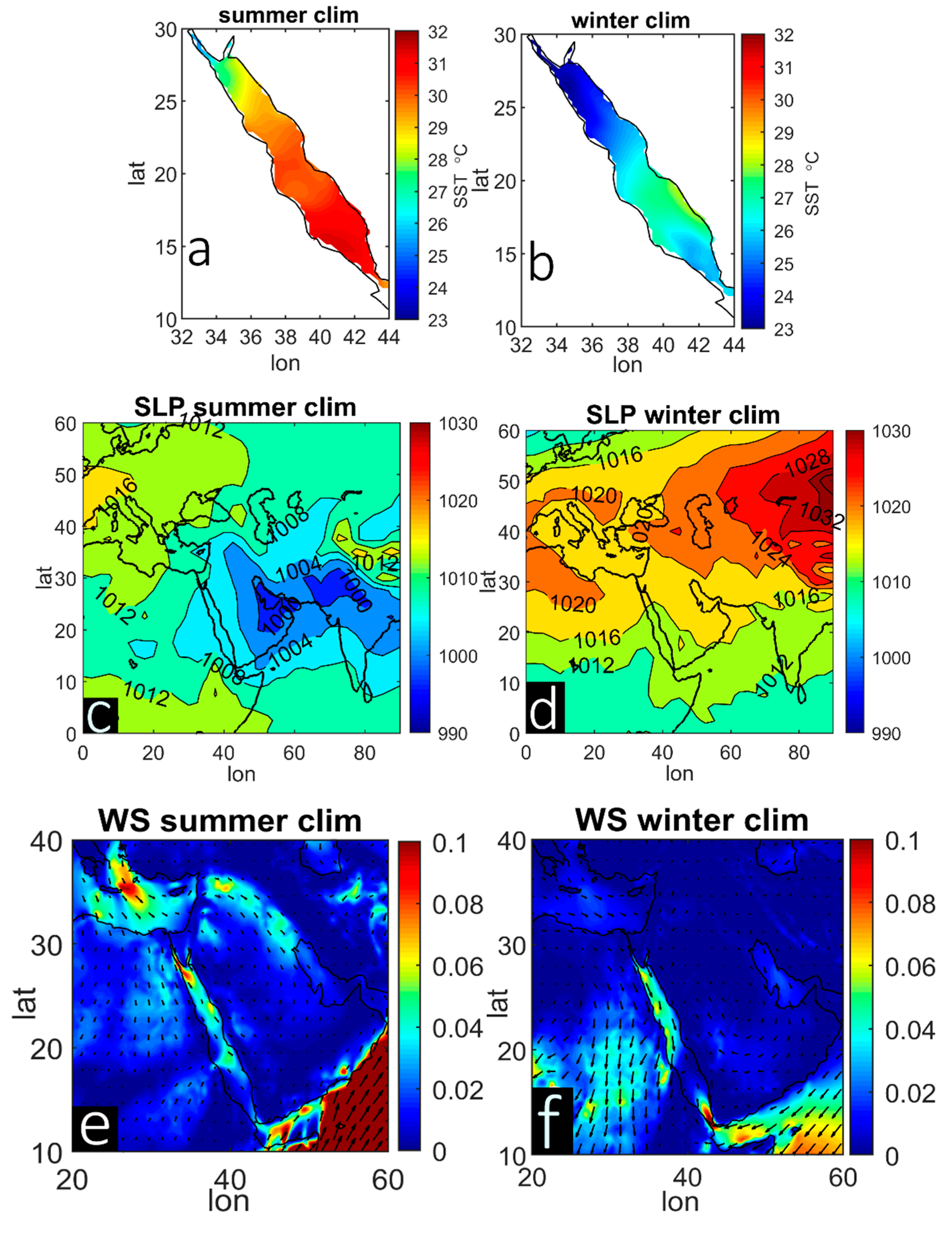
3.1. Climatological Features over the RS

Figure 2 shows the seasonal climatology of the SST, averaged over the summer and winter seasons of 1982–2018. The results show a strong meridional gradient of approximately 6 °C along a distance of 1500 km [29]. Summer values reaching 32 °C were observed over the southwestern part of the basin, while the lowest values of up to 26 °C were observed over the far northern end [30], especially on the Gulf of Suez (Figure 2a). This finding can be explained by the northerly winds that blow from relatively cold areas and cover the entire basin, which are associated with a negligible amount of water inflow from the Gulf of Aden during this season [31]. This gradient seems to be the factor triggering thermohaline-driven circulation, which is an important term in the RS circulation [32,33]. For the winter season (Figure 2b), a meridional gradient is also presented, but it is weak in comparison with the summer gradient, mainly due to the entrance of the relatively cold Gulf of Aden intermediate water [34]. In this situation, the maximum temperature shifts to the wind convergence zone in the central basin, where the wind is weak or calm [35,36].
To obtain background information about the atmospheric circulation that influences the extreme SST in the RS, we also present the climatology shown in the mean sea level pressure (SLP) and wind stress maps. In summer, the entire basin is affected by the westward extension of a monsoon low that crosses the RS and combines with the Sudan thermal low (or equatorial African low-pressure system in some studies), which is a favorable condition for the development of a clear pressure gradient in southern Europe (Figure 2c). During winter, the Sudan thermal low seems to be associated with the Red Rea Trough, which may play a key role in the projection of both central Asia and Azores high-pressure systems (Figure 2d). As a result of the pressure gradients, a wide blowing of northerly wind stress over the entire RS and surrounding area was observed during the summer season (Figure 2e). The same features were observed during the winter season (Figure 2f), which is associated with the blowing of southerly wind stress that converges in the central basin.

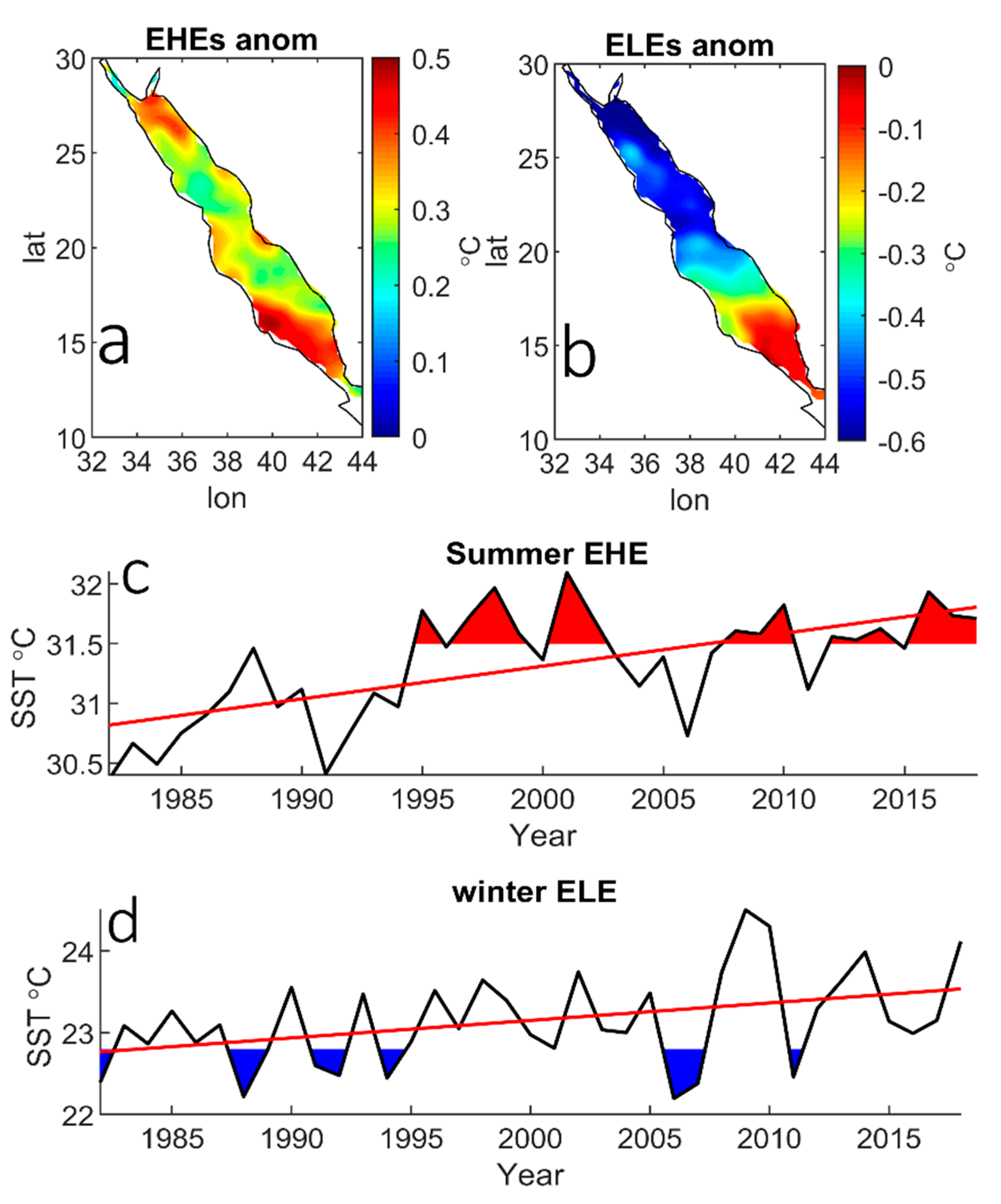
3.2. Spatial and Temporal EHEs and ELEs Variability

The spatial distributions of EHEs and ELEs anomalies are presented separately in Figure 3. Visually, the distributions of these two event types are completely different, as they have different atmospheric circulation. During EHEs, the RS experiences significant positive anomalies, up to 0.5 °C over the southern and northern ends, with less than this value in the center (Figure 3a). In addition to oceanic and atmospheric factors, the shallow area near the southern end seems to contribute to warming the water, since the land warming is much faster and vigorous than the water. During ELEs, the RS experiences significant negative anomalies of up to −0.6 °C over the northern end; this value gradually decreases toward the southern end (Figure 3b).
Figure 3c,d show the time series of the highest and lowest 5% of SST (37 years), including the years that have EHEs (red shaded area) and ELEs (blue shaded area) superimposed with their corresponding linear trends. The trend was fitted using least squares method, and the significance (99%) of the result was tested using the Mann–Kendall. It is clear that the EHEs that were greater than or equal to the threshold value (31.5 °C) started in the mid-1990s, with these events being absent prior to this period. The red line, which refers to the SST trend, indicates that the highest 5 % values including the EHEs are increasing by 0.027 °C year−1 (Figure 3c).
These results support the previous finding of Alawad et al. (2020) [19] that the whole RS has experienced a nonuniform warming trend since 1996, which has amplified over the northern half to reach 0.04 °C year−1—approximately 4 times higher than the global trend.
Figure 3d shows that the ELEs mostly occurred before 1996, being absent in the last 7 years. The trend analysis for the time series of the lowest 5 % including the ELEs shows an increasing tendency (0.027 °C year−1), which corresponds to the previous study showing that the annual mean SST (1982–2016) exhibited significant warming trend of 0.029 °C year−1 [20].
In brief, EHEs occur over the southern and northern ends, while ELEs over the northern ends only. Moreover, the positive trend in the SST indicates that warmer ocean climate conditions over the RS could be expected in the near future, increasing (decreasing) the EHEs (ELEs).

3.3. Physical Mechanisms

Atmospheric forcing on the ocean basins has been discussed on various spatial and temporal scales, since it can regulate air–sea heat fluxes, including the SST, and vice versa [24,37,38,39,40,41]. In this part, a composite analysis was carried out by averaging the corresponding SLP, wind stress, and net surface air–sea heat flux to determine the atmospheric pattern associated with each event.

3.3.1. SLP

SLP is considered an important atmospheric variable that is closely related to the general atmospheric circulation. Furthermore, it can give an indication about the surface air temperature, humidity, cloudiness, and wind flow in term of speed and direction.
Figure 4 shows the composite SLP maps corresponding to the EHEs and ELEs and their deviances from the climatology mean. The main conspicuous summer features are the monsoon low system and eastward extension of the Azores anticyclonic system over the southeastern Mediterranean Sea. The monsoonal trough has a westward propagation, which enables it to adjoin the equatorial African low belts, including the Red Sea Trough and Sudan thermal low. As a result of these synoptic features, the atmospheric circulation over the RS and adjoining regions is modulated by the pressure gradients between the monsoon low with less than 1002 hPa and the Azores high with more than 1014 hPa [37,42]. During EHEs, there is widespread negative SLPs that cover the extension area of both Azores and monsoon systems (Figure 4c). The most negative value (1 hPa) was found in the Azores high over the southeastern Mediterranean Sea. This situation decreases the above-mentioned pressure gradient, which weakens the wind advection to the RS and adjoining regions in the Middle East and Africa.
The most conspicuous winter features are the prominent existence of a westward extension of the Siberian anticyclone over eastern Asia (greater than 1032 hPa) jointly with the relatively weak eastward extension of the Azores high, covering a broad area from central Asia to southern Europe and North Africa. This synoptic condition creates a significant SLP gradient for transferring continental, cold, and dry air through the arid land mass around the northern part of the basin to the central part [23,32,43]. This gradient is clear from the existence of a strong positive SLP anomaly during ELEs over Turkey and the Mediterranean Sea (greater than 2 hPa) and it extends to central Africa. Charabi and Al-Hatrushi (2010) [44] considered these gradients to be important factors that modulate the winter rainfall (wet seasons) variability over northern Oman.
In brief, the intensity and the position variability of the main circulation pattern, namely the Siberian and Azores high and monsoon low, may trigger the occurrence as well as determine the intensity of EHEs and ELEs during the summer and winter periods, respectively.

3.3.2. Wind Stress

Figure 5 depicts the wind stress flow over the RS and surrounding area. From an atmospheric point of view, the winds follow the above spatial distributions of SLP in terms of speed and direction to form wind stress. For instance, the pressure gradient between the Azores high and monsoon low shapes the north-northwesterly wind over the entire RS and surrounding area during the summer season. In particular, for EHEs cases, the northerly wind stress experiences less than average values in all areas, including the RS. This means that the relatively cold air masses that are transferred from southern Europe to the southern RS are reduced during EHEs cases, which may be a possible factor that enhances the occurrence of EHEs. An interesting result is the intrusion of air masses (red box) from the mountain gap (Tokar gap) along the Sudanese coasts on the western RS side, with greater than average values (Figure 5b). These air masses are relatively warm and dry (locally called Hababai) and are mainly advected by the rain that is associated with the movement of the inter-tropical convergence zone that dominates eastern and central Africa during the summertime.
When entering the RS, it joins the northerly wind stress that governs the basin, and both move forward in a southerly direction. This mechanism may explain the occurrence of EHEs in the southern half of the basin during the summer period.
In brief, the combined effect of a relatively weaker than usual cold wind stress from the north and the intrusion of relatively stronger than usual warm air massed from the Tokar Gap are possible reasons for the occurrence of EHEs in the RS during the summer period.
Similarly, for the ELEs during the winter period (Figure 5d), the northerly wind stress strengthens over the northern half of the basin due to the strong pressure gradient shown in Figure 4c,d. At the same time, the stronger than usual wind stress coincides with the presence of less than usual southerly wind stress over the southern end, especially in Bab-Al-Mandab, where both winds converge in the central basin. This process may explain the occurrence of ELEs in the northern half of the basin. Moreover, the western land that surrounds the RS has experienced more wind stress than the eastern side, in particular Egypt and Sudan. This may be due to the eastern extension of the Azores high that makes the SLP center tilt to the west with reference to the RS. Previous studies have investigated the role of the atmospheric circulation in the RS circulation, and all have identified the immediate importance of the wind stress contribution on different spatial and temporal scales [30,31,45,46,47].
In brief, the strengthening of northerly wind stress, which advected cold air masses to the basin, coincides with the presence of less than usual southerly wind stress over the southern end, which transfers warm and humid air northward. This is a possible reason for the occurrence of ELEs in the RS during the winter period.
Taken together, the wind analysis emphasizes the vital role of atmospheric circulation in enhancing the occurrence as well as the frequency of EHEs and ELEs during the summer and winter periods, respectively.

3.3.3. The Net Surface Air–Sea Heat Flux

To understand in depth the transferring of atmospheric circulation signals to the sea, we showed the net air–sea heat fluxes anomalies during the EHEs and ELEs. Note that we present 8 years out of 10 and 15 years for the EHEs and ELEs, respectively, since the data span from 1984–2009. As the natural result of the presence of relatively warm air masses associated with less than average SLP and wind stress over the basin during the EHEs, the net surface air–sea heat flux is positive over the entire basin (heat gain from air to sea), with values up to 100 W m2 (not shown). These values produce positive anomalies mainly over the central basin (Figure 6a).
Conversely, during the ELEs, the net surface air–sea heat flux is negative over the entire basin (heat loss from sea to air), associated with a strong meridional gradient ranging from -1 W m2 in the south to over -200 W m2 in the north (not shown). These values represent less than average anomalies over the entire basin, except the southern end (Figure 6b). Interestingly, the far northern end seems to differ from the entire basin; this may be due to a complex physical process that enhances the intermediate- and deep-water formation. Further investigation using the re-analysis dataset and modelling approach can be more beneficial and a key point to understand the water formation process, which still remains unresolved [38].
In brief, the net surface air–sea heat flux results are consistent with the distinguished spatial distribution of SLP and wind stress for each event. The above average heat gain (loss) due to the presence of relatively warm (cold) air masses and less than (above) average SLP and wind stress is a possible reason for the occurrence of EHEs (ELEs).

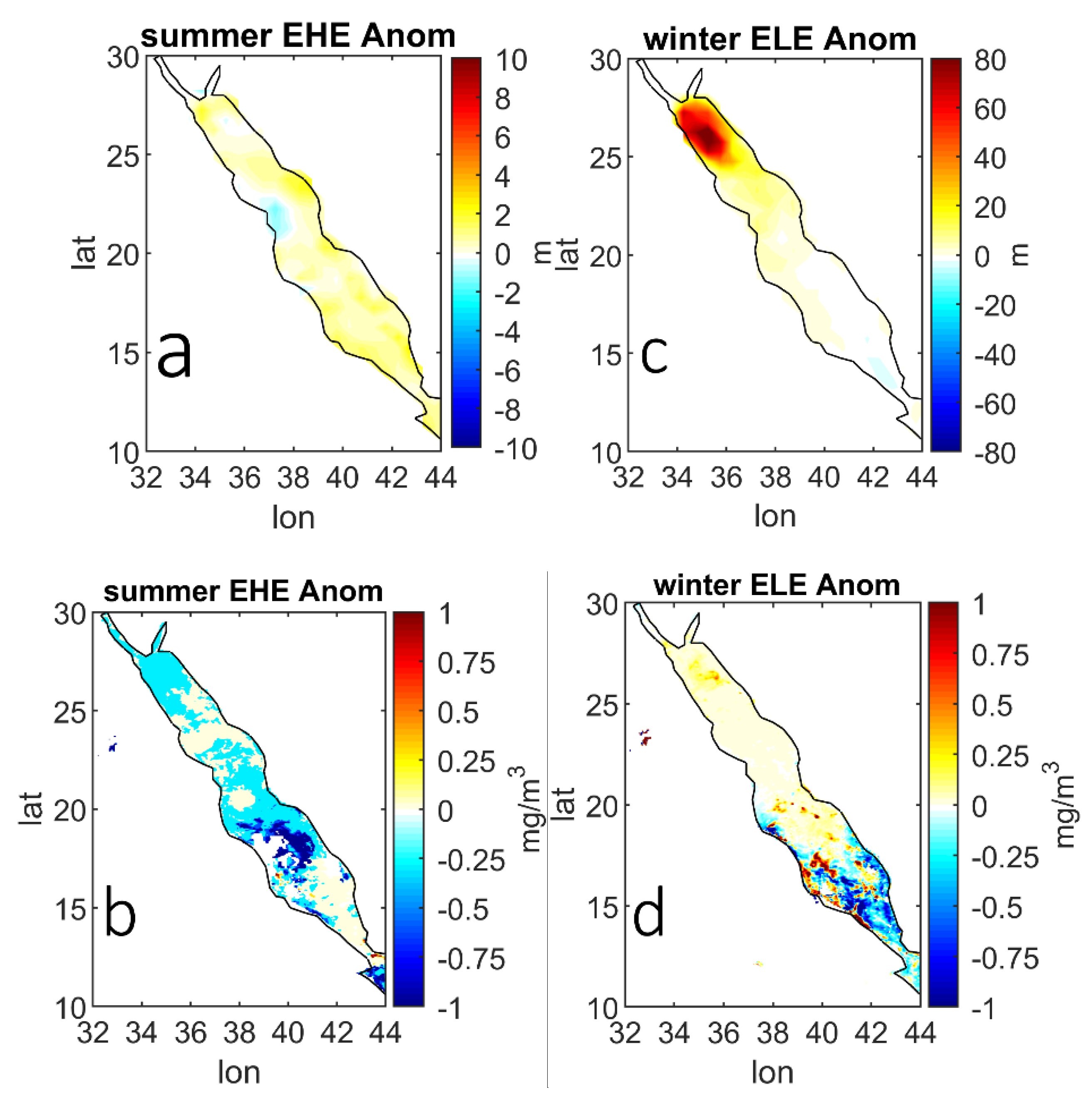
3.3.4. Associated MLD and Chl-a
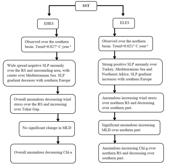
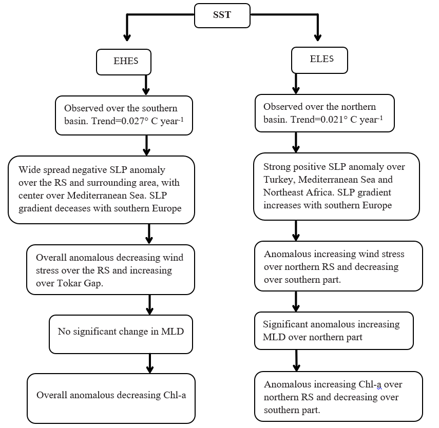
In order to understand the roles of atmospheric forcing and ocean physics variability on the biological ecosystem in the basin, we present the anomalies of MLD and Chl-a for EHEs and ELEs, which were calculated from the difference between composite maps of those events and their climatology values. The latter two maps are not shown in this analysis, and we only present the anomaly values for each event. The analysis included a nonsignificant anomaly in MLD for EHEs during the summer period (Figure 7a). The warmer the ocean surface and the more stable the stratified boundary layer, the shallower the MLD [48]; this is a well-known consequence of global warming [49]. The biological response during EHEs revealed a lower than average Chl-a concentration, especially in the central basin (Figure 7b). This result is in line with previous studies conducted on the RS [17,50]. The Chl-a concentration revealed a negative correlation [23], and reached its minimum values during heat wave events [20]. Comparable results have been observed in other ocean basins [51,52] and these have been linked with a warmer global climate [53]. Note that, due to the availability of data on Chl-a, which started to be recorded in 2003, we used 9 out of the 15 years available to analyze the EHEs during summer and only 3 out of 10 years to analyze the ELEs in the composite analysis.
Visually, the map of MLD anomalies looks somewhat similar to the spatial distribution of the SST during ELEs, since the area of the above average MLD corresponds to the area of the spatial distribution of the SST in the far northern end of the basin (compare Figure 7c and Figure 3c). The above average MLD is a natural impact of the unstable water column caused by the theoretical existence of dense water in the surface through the contribution of a less than average SST. A further natural impact is due to the occurrence of an above average Chl-a concentration over the same area as the water column mixing process increases. Triantafyllou et al. (2014) [54] and Sofianos and Johns (2003) [33] confirmed that vertical nutrient transport in this area is controlled by a deep convection or upwelling process. Conversely, the Chl-a concentration decreases over the southern entrance of the basin during ELEs (Figure 7d). This may be due to the wind stress weakening in the area, since Chl-a is advected by the southerly wind [18,55].
In brief, the analysis emphasizes links between the atmospheric circulations; ocean physical factors, including SST and MLD; and ocean fertility in terms of the Chl-a concentration.

4. Conclusions

This study explored the atmospheric circulation influencing the EHEs and ELEs over the RS, an area that has not yet been explored in previous studies. The question of how the physical processes of the atmosphere can affect the RS circulation is a highly important research topic, while the expected impact on the ecosystem is a challenge for near-future conditions. We focused on the summer and winter months only, since EHEs and ELEs are likely to take place during the hottest and coldest seasons of the year. The 37-year-long OISST record concludes that the EHEs (ELEs) observed over the southern (northern) basin have had a significant warming trend of 0.027 (0.021) °C year−1.
Based on the findings shown in this study (Figure 8), we propose a distinct type of atmospheric circulation for each event:
EHEs during the summer period mainly occur over the southern RS when the westward monsoonal trough is dominant and adjoins the equatorial African low belts, including the Red Sea Trough and Sudan thermal low. Negative SLP anomalies are widespread over the RS and surrounding area, centered over the Mediterranean Sea. The SLP gradient deceases in southern Europe. Overall, anomalous wind stress decreases over the RS and increases over the Tokar Gap area. Overall, anomalous Chl-a values decrease due to the stably stratified ocean boundary layer. This is a straightforward negative consequence of EHEs on the chlorophyll concentration.
ELEs during the winter period mainly occur over the northern RS when the westward extension of the Siberian anticyclone high adjoins the eastward extension of the Azores high. There is a strong positive SLP anomaly over Turkey, Mediterranean Sea, and northeast Africa. The SLP gradient significantly increases in southern Europe. The anomalous wind stress increases over northern RS and decreases over the southern part. The anomalous Chl-a values increase over northern RS due to a significant increase in anomalous MLD but decrease over the southern part. This is a straightforward positive consequence of the effect of ELEs on the chlorophyll concentration.
These results bring us a step closer toward the ability to report and understand the extreme SST variability seen in the RS. Our findings raise the possibility that a warmer global climate could make the RS ecosystem less productive following the tropical ocean [49,53], which provides a useful background on how a warmer climate scenario can alter marine ecosystems. Furthermore, there is a need to include paleo-biological data to allow us to closely look for RS productivity under past climatic conditions before simulating the effects of future climate change using climate models. In addition, it is important to understand that the atmospheric circulations that forced the RS and surrounding area climate, including EHEs and ELEs, are not local or regional phenomena but are a manifestation of superimposing remote impacts of the large-scale climatic mode from the tropical and polar regions [24,37,46,47,56,57,58].
Finally, sensitive experiments using ocean models could determine the exact roles of the SST and wind on RS productivity, enabling better projection of future climatic conditions, and this could help decision makers to mitigate the harmful impacts of global warming on the region.

Author Contributions

Conceptualization, methodology, software, formal analysis, writing—original draft preparation, K.A.A.; visualization, writing—review and editing, all authors. All authors have read and agreed to the published version of the manuscript.

Funding

This work was funded by the Deanship of Scientific Research (DSR), King Abdulaziz University, Jeddah, Saudi Arabia; grant number (D1441-46-150).

Acknowledgments

The authors would like to thank the DSR for their financial support and the teams of NOAA-OISST, ECMWF/ERA5, SODA-V3 and NASA Goddard Space Flight Center (Ocean Ecology Laboratory, Ocean Biology Processing Group- CHL-a) for making their data available. Furthermore, we thank the team at the HPC Center (Azizi Supercomputer)-King Abdulaziz University-Saudi Arabia. Finally, the authors would like to thank the four anonymous reviewers for their suggestions and comments.

Conflicts of Interest

The authors declare no conflict of interest.

References

  1. Gobler, C.J.; Doherty, O.M.; Hattenrath-Lehmann, T.K.; Griffith, A.W.; Kang, Y.; Litaker, R.W. Ocean warming since 1982 has expanded the niche of toxic algal blooms in the North Atlantic and North Pacific oceans. Proc. Natl. Acad. Sci. USA 2017, 114, 4975–4980. [Google Scholar] [CrossRef] [PubMed] [Green Version]
  2. Ainsworth, T.D.; Heron, S.F.; Ortiz, J.C.; Mumby, P.J.; Grech, A.; Ogawa, D.; Eakin, C.M.; Leggat, W. Climate change disables coral bleaching protection on the Great Barrier Reef. Science 2016, 352, 338–342. [Google Scholar] [CrossRef] [PubMed] [Green Version]
  3. Brander, K.M. Global fish production and climate change. Proc. Natl. Acad. Sci. USA 2007, 104, 19709–19714. [Google Scholar] [CrossRef] [Green Version]
  4. Harvell, C.D.; Kim, K.; Burkholder, J.M.; Colwell, R.R.; Epstein, P.R.; Grimes, D.J.; Hofmann, E.E.; Lipp, E.K.; Osterhaus, A.; Overstreet, R.M. Emerging marine diseases–climate links and anthropogenic factors. Science 1999, 285, 1505–1510. [Google Scholar] [CrossRef] [Green Version]
  5. Bindoff, N.L.; Cheung, W.W.; Kairo, J.G.; Arstegui, J.; Guinder, V.A.; Hallberg, R.; Hilmi, N.; Jiao, N.; Karim, M.S.; Levin, L. Changing ocean, marine ecosystems, and dependent communities. In IPCC Special Report on the Ocean and Cryosphere in a Changing Climate; United Nations Environment Programme: Nairobi, Kenya, 2019. [Google Scholar]
  6. IPCC. Climate Change 2013—The Physical Science Basis: Working Group I Contribution to the Fifth Assessment Report of the Intergovernmental Panel on Climate Change; Cambridge University Press: Cambridge, UK, 2014. [Google Scholar]
  7. Trenberth, K.E.; Dai, A.; Van Der Schrier, G.; Jones, P.D.; Barichivich, J.; Briffa, K.R.; Sheffield, J. Global warming and changes in drought. Nat. Clim. Chang. 2014, 4, 17–22. [Google Scholar] [CrossRef]
  8. Prospero, J.M.; Lamb, P.J. African droughts and dust transport to the Caribbean: Climate change implications. Science 2003, 302, 1024–1027. [Google Scholar] [CrossRef] [PubMed]
  9. Ban, N.; Schmidli, J.; Schär, C. Heavy precipitation in a changing climate: Does short-term summer precipitation increase faster? Geophys. Res. Lett. 2015, 42, 1165–1172. [Google Scholar] [CrossRef]
  10. Berg, N.; Hall, A. Increased interannual precipitation extremes over California under climate change. J. Clim. 2015, 28, 6324–6334. [Google Scholar] [CrossRef]
  11. Cane, M.A.; Clement, A.C.; Kaplan, A.; Kushnir, Y.; Pozdnyakov, D.; Seager, R.; Zebiak, S.E.; Murtugudde, R. Twentieth-century sea surface temperature trends. Science 1997, 275, 957–960. [Google Scholar] [CrossRef] [PubMed] [Green Version]
  12. Collins, M.; Knutti, R.; Arblaster, J.; Dufresne, J.-L.; Fichefet, T.; Friedlingstein, P.; Gao, X.; Gutowski, W.J.; Johns, T.; Krinner, G. Long-term climate change: Projections, commitments and irreversibility. In Climate Change 2013—The Physical Science Basis: Contribution of Working Group I to the Fifth Assessment Report of the Intergovernmental Panel on Climate Change; Cambridge University Press: Cambridge, UK, 2013; pp. 1029–1136. [Google Scholar]
  13. Xie, S.-P.; Deser, C.; Vecchi, G.A.; Collins, M.; Delworth, T.L.; Hall, A.; Hawkins, E.; Johnson, N.C.; Cassou, C.; Giannini, A. Towards predictive understanding of regional climate change. Nat. Clim. Chang. 2015, 5, 921. [Google Scholar] [CrossRef]
  14. Pithan, F.; Mauritsen, T. Arctic amplification dominated by temperature feedbacks in contemporary climate models. Nat. Geosci. 2014, 7, 181. [Google Scholar] [CrossRef]
  15. Belkin, I.M. Rapid warming of large marine ecosystems. Prog. Oceanogr. 2009, 81, 207–213. [Google Scholar] [CrossRef]
  16. Hoegh-Guldberg, O.; Cai, R.; Poloczanska, E.S.; Brewer, P.G.; Sundby, S.; Hilmi, K.; Barros, V.R.; Field, C.B.; Dokken, D.J.; Mastrandrea, M.D. Climate Change 2014: Impacts, Adaptation, and Vulnerability Part B: Regional Aspects; Cambridge University Press: Cambridge, UK, 2014. [Google Scholar]
  17. Chaidez, V.; Dreano, D.; Agusti, S.; Duarte, C.M.; Hoteit, I. Decadal trends in Red Sea maximum surface temperature. Sci. Rep. 2017, 7, 8144. [Google Scholar] [CrossRef] [PubMed] [Green Version]
  18. Raitsos, D.E.; Yi, X.; Platt, T.; Racault, M.-F.; Brewin, R.J.; Pradhan, Y.; Papadopoulos, V.P.; Sathyendranath, S.; Hoteit, I. Monsoon oscillations regulate fertility of the Red Sea. Geophys. Res. Lett. 2015, 42, 855–862. [Google Scholar] [CrossRef] [Green Version]
  19. Alawad, K.A.; Al-Subhi, A.M.; Alsaafani, M.A.; Turki, M. Alraddad Decadal variability and recent summer warming amplification of sea surface temperature in the Red Sea. PLoS ONE 2020, submitted. [Google Scholar]
  20. Shaltout, M. Recent sea surface temperature trends and future scenarios for the Red Sea. Oceanologia 2019, 61, 484–504. [Google Scholar] [CrossRef]
  21. Roik, A.; Roder, C.; Röthig, T.; Voolstra, C.R. Spatial and seasonal reef calcification in corals and calcareous crusts in the central Red Sea. Coral Reefs 2016, 35, 681–693. [Google Scholar] [CrossRef] [Green Version]
  22. Cantin, N.E.; Cohen, A.L.; Karnauskas, K.B.; Tarrant, A.M.; McCorkle, D.C. Ocean warming slows coral growth in the central Red Sea. Science 2010, 329, 322–325. [Google Scholar] [CrossRef] [Green Version]
  23. Eladawy, A.; Nadaoka, K.; Negm, A.; Abdel-Fattah, S.; Hanafy, M.; Shaltout, M. Characterization of the northern Red Sea’s oceanic features with remote sensing data and outputs from a global circulation model. Oceanologia 2017, 59, 213–237. [Google Scholar] [CrossRef]
  24. Karnauskas, K.B.; Jones, B.H. The interannual variability of sea surface temperature in the Red Sea from 35 years of satellite and in situ observations. J. Geophys. Res. Oceans 2018, 123, 5824–5841. [Google Scholar] [CrossRef]
  25. Reynolds, R.W.; Smith, T.M.; Liu, C.; Chelton, D.B.; Casey, K.S.; Schlax, M.G. Daily high-resolution-blended analyses for sea surface temperature. J. Clim. 2007, 20, 5473–5496. [Google Scholar] [CrossRef]
  26. Worley, S.J.; Woodruff, S.D.; Reynolds, R.W.; Lubker, S.J.; Lott, N. ICOADS release 2.1 data and products. Int. J. Climatol. J. R. Meteorol. Soc. 2005, 25, 823–842. [Google Scholar] [CrossRef]
  27. Carton, J.A.; Chepurin, G.A.; Chen, L. SODA3: A new ocean climate reanalysis. J. Clim. 2018, 31, 6967–6983. [Google Scholar] [CrossRef]
  28. NASA Goddard Space Flight Center; Ocean Biology Processing Group. Sea-Viewing Wide Field-of-View Sensor (SeaWiFS) Ocean Color Data; NASA Ocean Biology Distibuted Active Archive Center (NASA OB.DAAC): Greenbelt, MD, USA, 2014. [Google Scholar] [CrossRef]
  29. Al-Subhi, A.M.; Taqi, A.M. Remotely Sensed Sea Surface Temperature Variations in the Southern Red Sea in Relation to Some Meteorological Variables. J. King Abdulaziz Univ. 2010, 21, 33. [Google Scholar]
  30. Al-Subhi, A.M.; Al-Aqsum, M.M. Temporal and Spatial Variations of Remotely Sensed Sea Surface Temperature in the Northern Red Sea. J. King Abdulaziz Univ. Mar. Sci 2008, 19, 61–74. [Google Scholar] [CrossRef]
  31. Sofianos, S.S.; Johns, W.E. Wind induced sea level variability in the Red Sea. Geophys. Res. Lett. 2001, 28, 3175–3178. [Google Scholar] [CrossRef]
  32. Felis, T.; Mudelsee, M. Pacing of Red Sea deep water renewal during the last centuries. Geophys. Res. Lett. 2019, 46, 4413–4420. [Google Scholar] [CrossRef] [Green Version]
  33. Sofianos, S.S.; Johns, W.E. An oceanic general circulation model (OGCM) investigation of the Red Sea circulation: 2. Three-dimensional circulation in the Red Sea. J. Geophys. Res. Oceans 2003, 108, 3066. [Google Scholar] [CrossRef] [Green Version]
  34. Al Saafani, M.A.; Shenoi, S.S.C. Water masses in the Gulf of Aden. J. Oceanogr. 2007, 63, 1–14. [Google Scholar] [CrossRef]
  35. Ali, E.B.; Churchill, J.H.; Barthel, K.; Skjelvan, I.; Omar, A.M.; de Lange, T.E.; Eltaib, E.B. Seasonal variations of hydrographic parameters off the Sudanese coast of the Red Sea, 2009–2015. Reg. Stud. Mar. Sci. 2018, 18, 1–10. [Google Scholar] [CrossRef]
  36. Al-Subhi, A.M.; Taqi, A.M. Surface Circulation of the Southern Red Sea as Inferred From AVHRR Data. J. King Abdulaziz Univ. 2014, 25, 121. [Google Scholar] [CrossRef]
  37. Abualnaja, Y.; Papadopoulos, V.P.; Josey, S.A.; Hoteit, I.; Kontoyiannis, H.; Raitsos, D.E. Impacts of climate modes on air–sea heat exchange in the Red Sea. J. Clim. 2015, 28, 2665–2681. [Google Scholar] [CrossRef] [Green Version]
  38. Papadopoulos, V.P.; Abualnaja, Y.; Josey, S.A.; Bower, A.; Raitsos, D.E.; Kontoyiannis, H.; Hoteit, I. Atmospheric forcing of the winter air–sea heat fluxes over the northern Red Sea. J. Clim. 2013, 26, 1685–1701. [Google Scholar] [CrossRef] [Green Version]
  39. Kontoyiannis, H.; Papadopoulos, V.; Kazmin, A.; Zatsepin, A.; Georgopoulos, D. Climatic variability of the sub-surface sea temperatures in the Aegean-Black Sea system and relation to meteorological forcing. Clim. Dyn. 2012, 39, 1507–1525. [Google Scholar] [CrossRef]
  40. Papadopoulos, V.P.; Kontoyiannis, H.; Ruiz, S.; Zarokanellos, N. Influence of atmospheric circulation on turbulent air-sea heat fluxes over the Mediterranean Sea during winter. J. Geophys. Res. Oceans 2012, 117. [Google Scholar] [CrossRef]
  41. Patzert, W.C. Wind-induced reversal in Red Sea circulation. In Deep Sea Research and Oceanographic Abstracts; Elsevier: Amsterdam, The Netherlands, 1974; Volume 21, pp. 109–121. [Google Scholar]
  42. Jiang, H.; Farrar, J.T.; Beardsley, R.C.; Chen, R.; Chen, C. Zonal surface wind jets across the Red Sea due to mountain gap forcing along both sides of the Red Sea. Geophys. Res. Lett. 2009, 36. [Google Scholar] [CrossRef] [Green Version]
  43. Ionita, M.; Felis, T.; Lohmann, G.; Rimbu, N.; Pätzold, J. Distinct modes of East Asian Winter Monsoon documented by a southern Red Sea coral record. J. Geophys. Res. Oceans 2014, 119, 1517–1533. [Google Scholar] [CrossRef] [Green Version]
  44. Charabi, Y.; Al-Hatrushi, S. Synoptic aspects of winter rainfall variability in Oman. Atmos. Res. 2010, 95, 470–486. [Google Scholar] [CrossRef]
  45. Zubier, K.M.; Eyouni, L.S. Investigating the Role of Atmospheric Variables on Sea Level Variations in the Eastern Central Red Sea Using an Artificial Neural Network Approach. Oceanologia 2020. [Google Scholar] [CrossRef]
  46. Alawad, K.A.; Al-Subhi, A.M.; Alsaafani, M.A.; Alraddadi, T.M.; Ionita, M.; Lohmann, G. Large-Scale Mode Impacts on the Sea Level over the Red Sea and Gulf of Aden. Remote Sens. 2019, 11, 2224. [Google Scholar] [CrossRef] [Green Version]
  47. Alawad, K.; Alsaafani, M.A.; Al-Subhi, A.M.; Alraddadi, T.M. Signatures of Tropical Climate Modes on the Red Sea and Gulf of Aden Sea Level; NISCAIR-CSIR: New Delhi, India, 2017. [Google Scholar]
  48. Somavilla, R.; González-Pola, C.; Fernández-Diaz, J. The warmer the ocean surface, the shallower the mixed layer. How much of this is true? J. Geophys. Res. Oceans 2017, 122, 7698–7716. [Google Scholar] [CrossRef]
  49. Behrenfeld, M.J.; O’Malley, R.T.; Siegel, D.A.; McClain, C.R.; Sarmiento, J.L.; Feldman, G.C.; Milligan, A.J.; Falkowski, P.G.; Letelier, R.M.; Boss, E.S. Climate-driven trends in contemporary ocean productivity. Nature 2006, 444, 752–755. [Google Scholar] [CrossRef] [PubMed]
  50. Maor-Landaw, K.; Karako-Lampert, S.; Ben-Asher, H.W.; Goffredo, S.; Falini, G.; Dubinsky, Z.; Levy, O. Gene expression profiles during short-term heat stress in the red sea coral Stylophora pistillata. Glob. Chang. Biol. 2014, 20, 3026–3035. [Google Scholar] [CrossRef] [PubMed] [Green Version]
  51. Bai, Y.; He, X.; Yu, S.; Chen, C.-T.A. Changes in the Ecological Environment of the Marginal Seas along the Eurasian Continent from 2003 to 2014. Sustainability 2018, 10, 635. [Google Scholar] [CrossRef] [Green Version]
  52. Caputi, N.; Jackson, G.; Pearce, A. The Marine Heat Wave off Western Australia During the Summer of 2010/11: 2 Years on; Fisheries Research Division, Western Australian Fisheries and Marine: North Beach, Australia, 2014. [Google Scholar]
  53. Doney, S.C. Plankton in a warmer world. Nature 2006, 444, 695–696. [Google Scholar] [CrossRef] [PubMed] [Green Version]
  54. Triantafyllou, G.; Yao, F.; Petihakis, G.; Tsiaras, K.P.; Raitsos, D.E.; Hoteit, I. Exploring the Red Sea seasonal ecosystem functioning using a three-dimensional biophysical model. J. Geophys. Res. Oceans 2014, 119, 1791–1811. [Google Scholar] [CrossRef] [Green Version]
  55. Raitsos, D.E.; Pradhan, Y.; Brewin, R.J.; Stenchikov, G.; Hoteit, I. Remote sensing the phytoplankton seasonal succession of the Red Sea. PLoS ONE 2013, 8. [Google Scholar] [CrossRef] [Green Version]
  56. Ehsan, M.A.; Nicolì, D.; Kucharski, F.; Almazroui, M.; Tippett, M.K.; Bellucci, A.; Ruggieri, P.; Kang, I.-S. Atlantic Ocean influence on Middle East summer surface air temperature. NPJ Clim. Atmos. Sci. 2020, 3, 1–8. [Google Scholar] [CrossRef] [Green Version]
  57. Krokos, G.; Papadopoulos, V.P.; Sofianos, S.S.; Ombao, H.; Dybczak, P.; Hoteit, I. Natural climate oscillations may counteract Red Sea warming over the coming decades. Geophys. Res. Lett. 2019, 46, 3454–3461. [Google Scholar] [CrossRef] [Green Version]
  58. Shanas, P.R.; Aboobacker, V.M.; Albarakati, A.M.; Zubier, K.M. Climate driven variability of wind-waves in the Red Sea. Ocean Model. 2017, 119, 105–117. [Google Scholar] [CrossRef]
Figure 1. Map of the Red Sea basin associated with bathymetry in meters (m).
Remotesensing 12 02227 g001
Figure 2. Summer and winter climatology of the sea surface temperature (SST) in °C (a,b), sea level pressure (SLP) in hPa (c,d), and wind stress magnitude in Pa (shaded color) and wind stress direction (black arrows) (e,f).
Remotesensing 12 02227 g002
Figure 3. Spatial SST anomalies in °C for EHEs and ELEs (a,b), and the time series of the highest (lowest) 5% SST events including EHEs (ELEs) superimposed with their corresponding linear trends (c,d).
Remotesensing 12 02227 g003
Figure 4. Composite SLP (a) and associated anomaly values (b) in hPa for EHEs. Same for (c) and (d), but for ELEs.
Remotesensing 12 02227 g004
Figure 5. Composite wind stress (a) and associated anomaly values (b) in Pa for EHEs. Same for (c) and (d) but for ELEs. The shaded color represents the magnitude of the wind stress, while the black arrows in (a) and (c) represents the direction.
Remotesensing 12 02227 g005
Figure 6. Composite anomalies of the net surface air–sea heat flux in w/m2 for EHEs (a) and ELEs (b).
Remotesensing 12 02227 g006
Figure 7. Composite anomalies of the mixed layer depth in m (a) and Chl-a concentration in mg/m3 (b) for EHEs. Same for (c) and (d) but for ELEs.
Remotesensing 12 02227 g007
Figure 8. Schematic diagram for the occurrence of EHEs and ELEs due to atmospheric forcing.
Remotesensing 12 02227 g008
Table 1. Extreme high events (EHEs) and extreme low events (ElEs) during summer and winter periods.
Winter ELEsSummer EHEs
19821995
19881997
19891998
19911999
19922001
19942002
19952008
20062009
20072010
20112012
-2013
-2014
-2016
-2017
-2018
1015

